Jan 25, 2018 - complements this by showing the expected rank of persistent homology with fixed persistence. 1. arXiv:1801.08376v1 [math.AT] 25 Jan 2018 ...
ˇ PERSISTENT BETTI NUMBERS OF RANDOM CECH COMPLEXES
arXiv:1801.08376v1 [math.AT] 25 Jan 2018
ULRICH BAUER AND FLORIAN PAUSINGER ˇ Abstract. We study the persistent homology of random Cech complexes. Generalizing a method of Penrose for studying random geometric graphs, we first describe an appropriate theoretical framework in which we can state and address our main questions. Then we define ˇ the kth persistent Betti number of a random Cech complex and determine its asymptotic order in the subcritical regime. This extends a result of Kahle on the asymptotic order of the ordinary kth Betti number of such complexes to the persistent setting.
1. Introduction 1.1. Motivation. In this paper we study the persistent homology of random geometric complexes, which are simplicial complexes built on the points of a Poisson point process in dˇ dimensional Euclidean space. In particular, we focus on Cech complexes, which are homotopy equivalent to a union of balls of the same radius centered at the points; however, analogous results can also be obtained for Vietoris–Rips complexes using essentialy the same arguments. Our work is motivated by recent results on the topology of random geometric complexes (see [1] for a survey) as well as topological data analysis, an emerging field that received increasing attention over the last years. In this context, point cloud data is analyzed with methods from persistent homology. The goal of a statistical interpretation of the results requires a probabilistic null hypothesis to compare the results to. Thus, it is of utmost importance to understand the persistent homology of randomly sampled point sets. We provide results in this direction, drawing motivation for our investigations on results of Kahle [4] on the homology of geometric complexes built from random point sets. In that paper, Kahle determined ˇ the expected Betti numbers of random Cech and Vietoris–Rips complexes asymptotically (as the number of points, n, goes to ∞), and identified four different regimes for the radius parameter rn , in dependence of n, with qualitatively different behavior. Our main contribution is twofold. First, we describe an appropriate theoretical framework in which we can state and address our main questions, reformulating central results of Penrose [7] about random geometric graphs in a more general setting of geometric properties. In a second step, we extend the results obtained by Kahle for the subcritical regime, i.e., for radii rn with rn d n → 0 as n → ∞. In particular, we determine the asymptotic order of the expected ˇ kth persistent Betti number of a random Cech complex, recovering the original result of Kahle on the ordinary kth Betti number of such complexes as a special case. The persistent homology of random geometric complexes has also received attention in recent work by Bobrowski, Kahle, and Skraba [2], who show the asymptotic order of the expected maximum persistence arising in a filtration of geometric complexes. Our work complements this by showing the expected rank of persistent homology with fixed persistence. 1
2
U. BAUER AND F. PAUSINGER
1.2. Preliminaries. Let P = {x1 , . . . , xN } be a collection of points in Rd and let r > 0. The ˇ Cech complex Cechr (P ) is a simplicial complex defined as � � \ B r (x) 6= ∅ , Cechr (P ) = Q ⊆ P | x∈Q
where B r (x) denotes the closed ball of radius r centered at x. By the Nerve Theorem, Cechr (P ) is homotopy-equivalent to the union of balls [ B r (P ) = B r (x) x∈P
of radius r centered at the points in P . Furthermore, let λ : Rd → [0, ∞) be a bounded measurable function. A Poisson process with intensity function λ is a point process P in Rd with the property that Rfor a Borel set A ⊆ Rd , the random variable P(A) is Poisson distributed with parameter A λ(x) dx whenever this integral is finite, and if A1 , . . . , Am are disjoint Borel subsets of Rd , then the variables P(Ai ), 1 ≤ i ≤ m, are mutually independent; see [5, 7]. In the context of this paper, we are interested in a Poisson point process on Rd with intensity function x 7→ nf (x), where n ∈ N, x ∈ Rd and f is a bounded probability density function. One concrete way of constructing such a Poisson point process is given as follows. Let f be a bounded probability density function on Rd , and let x1 , x2 , . . . be independent and identically distributed d-dimensional random variables with common density f . For given n > 0, let Nn be a Poisson random variable, independent of {x1 , x2 , . . .}, and let Pn := {x1 , x2 , . . . , xNn }. It is shown in [7, Proposition 1.5] that Pn is indeed a Poisson point process on Rd with ˇ intensity x 7→ nf (x). We call a Cech complex that is built from the random set Pn a random ˇ Cech complex. We note that in our particular setting in Section 3 and Section 4 working with a Poisson point process Pn offers some technical advantages over working with a random set Xn = {x1 , . . . , xn } of fixed size, also called binomial point process. However, the results in Section 2 are most easily obtained for a binomial process Xn . Therefore, we briefly recall what is known as Palm theory for Poisson processes; see [7, Section 1.6 and 1.7] for a thorough discussion of this issue. Theorem 1.1 ([7], Theorem 1.6). Let n > 0. Suppose p ∈ N and suppose h(Y, X) is a bounded measurable function defined on all pairs of the form (Y, X) with X being a finite subset of Rd and Y a subset of X, satisfying h(Y, X) = 0 unless Y has p elements. Then X np E (h(Xp , Xp ∪ Pn )) , E h(Y, Pn ) = p! Y ⊆Pn
where the sum on the left-hand side is over all subsets Y of the Poisson point process Pn , and the binomial point process set Xp is assumed to be independent of Pn .
ˇ PERSISTENT BETTI NUMBERS OF RANDOM CECH COMPLEXES
3
1.3. Results. Throughout this paper, we use the Landau symbols to describe the asymptotic growth of functions. In particular, we write f ∈ O(g) if there is a constant C > 0 and an x0 > 0 such that |f (x)| ≤ C · |g(x)| for all x > x0 . Similarly, we write f ∈ Ω(g) if there is a constant c > 0 and an x0 > 0 such that c · |g(x)| ≤ |f (x)| for all x > x0 . And finally, we write f ∈ Θ(g) if there are constants C > c > 0 and x0 > 0 such that c · |g(x)| ≤ |f (x)| ≤ C · |g(x)| for all x > x0 . We generalize the results of Kahle [4] in the subcritical regime, i.e., for radii rn satisfying rn d n → 0 as n → ∞. We fix a parameter ϑ ≥ 1 and define the kth ϑ-persistent Betti number of the inclusion map Cechr (P ) ,→ Cechϑr (P ) for a point set P ⊂ Rd as βkϑ (P, r) := rank Hk (Cechr (P ) ,→ Cechϑr (P )), where Hk denotes the kth homology with coefficients in a fixed field K. Consequently, setting ϑ = 1, we obtain the usual Betti numbers βk (P, r) := rank Hk (Cechr (P )). We briefly discuss the related case for integer coefficients in the final section. Our main result provides asymptotic bounds for βkϑ (Pn , rn ) for radii rn in the subcritical regime. Theorem 1.2. Let Pn be as defined above and let ϑ ≥ 1, d ≥ 2 and 1 ≤ k ≤ d − 1. Let rn d n → 0 for n → ∞. The expected kth ϑ-persistent Betti number of the inclusion Cechrn (Pn ) ,→ Cechϑrn (Pn ) satisfies � � E(βkϑ (Pn , rn )) ∈ Θ n(rn d n)(m−1) as n → ∞, where m = m(ϑ, k) is an integer depending on ϑ and k. See Fig. 1 for an example with parameters chosen such that the persistent Betti number behaves as Θ(1). For ϑ = 1, we have m(1, k) = k + 2, and the above theorem matches a result ˇ of Kahle [4, Theorem 3.2] about the expected Betti number of Cech complexes: ˇ Corollary 1.3. The expected kth Betti number of a random Cech complex Cechr (Pn ) satisfies � � E(βk (Pn , rn )) ∈ Θ n(rn d n)(k+1) , as n → ∞. The proof of Theorem 1.2 makes essential use of a method used by Penrose to study random geometric graphs [7]. We generalize this method to the setting of finite geometric properties in Section 2, and we apply it in Section 3 to prove the asymptotic lower bound. In Section 4 we show the upper bound to complete the proof of Theorem 1.2, and we conclude our paper with final remarks and open problems in Section 5. 2. The method of Penrose The goal of this section is to reformulate two technical results of Penrose [7, Propositions 3.1 and 3.2] on the expectation of connected subgraph and component counts in random geometric graphs. In particular, we show that the proof method of Penrose allows us to state these results in a more general way, which we use to prove Theorem 1.2 in the next sections.
4
U. BAUER AND F. PAUSINGER
Figure 1. Examples illustrating Theorem 1.2. Unions of balls of radius rn (dark) and ϑrn (light) around point sets Pn of cardinality n = 100 (left), n = 1000 (center), n = 10000 (right), drawn uniformly at random from [−1, 1]2 , with parameters chosen such that E(βkϑ (Pn , rn )) ∈ Θ(1); specifically, d = 2, ϑ = 1.4, k = 1, m = m(ϑ, k) = 4, m and rn = cnq with c = 2.6, q = − d(m−1) . In each of the three instances, we have ϑ βk (Pn , rn ) = 1.
2.1. Finite geometric properties. Let P(Rd ) denote the power set of Rd . A family of indicator functions gr,p : P(Rd ) → {0, 1}, with p ∈ N and 0 < r ∈ R, is called a finite geometric property if (i) gr,p is translation invariant, i.e., gr,p (Y ) = gr,p (Y + t) for all t ∈ Rd ; (ii) gr,p is scaling equivariant, i.e., gr,p (Y ) = gλr,p (λY ) for all λ ∈ R; (iii) gr,p is finite, i.e., |Y | = 6 p =⇒ gr,p (Y ) = 0 for every Y ⊆ Rd ; in other words gr,p is zero unless Y has p elements; (iv) gr,p is local, i.e., any Y ⊂ Rd with gr,p (Y ) = 1 satisfies diam Y ≤ C · r · p for some constant C. The first example motivating our definition is the finite geometric property of point configurations inducing a geometric graph isomorphic to a given connected graph Γ. To this end, let G(P, r) denote the geometric graph on P at scale r, containing an edge precisely for every pair of points with distance at most r. Define an indicator function for all finite Y ⊂ Rd by Hr,p (Y ) := 1|Y |=p · 1G(Y,r)∼ =Γ . This indicator function checks whether the geometric graph built on the points of the finite set Y is isomorphic to Γ, and satisfies all required properties. The results of Penrose [7] concern the special case of connected geometric graphs. In our framework, we replace the condition that the geometric graph built on a finite set Y is isomorphic to a connected graph by the above more general condition of being a local property. Note that isomorphism to a given connected graph Γ is a local property since connectivity enforces the vertex set to have diameter bounded by r · p. The generalization to local properties enables us to study a wider class of indicator functions. For example, 0 Hr,p (Y ) := 1|Y |=p · 1β0 (Y,r)=p · 1diam Y ≤r·p ,
for all finite Y ⊂ Rd is a geometric property, which checks whether Y consists of p points such that all pairwise distances are greater than r but less than or equal to r · p.
ˇ PERSISTENT BETTI NUMBERS OF RANDOM CECH COMPLEXES
5
We now turn to a particular class of finite geometric properties, which are very natural in certain settings. In particular, they appear whenever we are interested in a property that not only concerns the points of a subset Y ⊆ X but also the elements of the complement X \ Y . We call a family of indicator functions hr,p : P(Rd ) × P(Rd ) → {0, 1} for p ∈ N and 0 < r ∈ R a finite geometric subset property if (i) hr,p (Y, X) = 0 whenever Y 6⊆ X; ˜ r (Y, X) · gr,p (Y ), where h ˜ r is an (ii) hr,p (Y, X) can be written as a product hr,p (Y, X) = h indicator function and gr,p is a finite geometric property; (iii) hr,p is translation invariant, i.e., hr,p (Y, X) = hr,p (Y + t, X + t) for all t ∈ Rd ; (iv) hr,p is scaling equivariant, i.e., hr,p (Y, X) = hλr,p (λY, λX) for all λ ∈ R; (v) hr,p is finite, i.e., |Y | = 6 p =⇒ hr,p (Y, X) = 0 for every Y ⊆ Rd . Note that (ii) implies that hr,p is local since gr,p is assumed local as a finite geometric property. In contrast to just a geometric property, which depends only on the point set Y , a geometric subset property can also depend on the other points in the larger set X. Example 2.1. As an example which will also be used later, we say a subset Y ⊆ X forms ˇ an isolated component in the Cech complex Cechs (X) of a point set X if the union of balls with radius s centered at the points of Y has an empty intersection with the union of balls centered at points of X \ Y and if β0 (Y, s) = 1. Then � 1 if |Y | = p and Y forms an isolated component in Cechr (X), compr,p (Y, X) = 0 otherwise, is a finite geometric subset property, which can be written as a product compr,p (Y, X) = sepr (Y, X) · connr,p (Y ), where the indicator function sepr is given by ( 1 if d(x, y) > 2r for all x ∈ X \ Y and y ∈ Y, sepr (Y, X) = 0 otherwise. and the finite geometric property connr,p is given by ( 1 if |Y | = p and β0 (Y, r) = 1, connr,p (Y ) = 0 otherwise. 2.2. Subset counts. We are interested in the expected number of occurrences of a finite geometric property in a random point set, i.e., the number of subsets satisfying the property. Penrose [7] states our Propositions 2.2 and 2.3 in the setting of subgraph counts. His proofs, however, apply to our more general setting with only minor modifications, as we will now show. For a finite P ⊂ Rd we define X X (1) Count(gr,p , P ) := gr,p (Y ) and RelativeCount(hr,p , P ) := hr,p (Y, P ), Y ⊆P
Y ⊆P
which count the occurrences of a finite geometric property gr,p and of a finite geometric subset property hr,p in the set P , respectively.
6
U. BAUER AND F. PAUSINGER
Considering the random setting of a Poisson point process Pn on Rd with intensity function x 7→ nf (x), where f is a bounded probability density function on Rd , and given a finite geometric property gr,p , we define Z Z 1 p g1,p ({0, x1 , . . . , xp−1 }) d(x1 , . . . , xp−1 ). f (x) dx (2) µg1,p := p! Rd (Rd )p−1 Note that the boundedness of f implies that f (x)p is integrable: Let f ≤ C for some constant C and assume by induction that f p−1 is integrable. Then f p ≤ f p−1 · C is integrable. Furthermore, the condition that gr,p is local implies that g1,p ({0, x1 , . . . , xp−1 }) is integrable since it is bounded and zero outside of a bounded region, a ball centered at 0 with radius equal to the diameter bound from the locality condition. We obtain the following asymptotic result: Proposition 2.2 (see [7], Proposition 3.1). Suppose that gr,p is a finite geometric property for p ≥ 2 that occurs with positive probability for Xp and for all sufficiently small r > 0. Let limn→∞ rn = 0. Then E(Count(grn ,p , Xn )) E(Count(grn ,p , Pn )) = lim = µg1,p . (p−1) d n→∞ n→∞ n(rn n) n(rn d n)(p−1) lim
Proof. We slightly modify the proof of [7, Proposition 3.1]. The goal is to highlight that we can replace the subgraph counts of Penrose by our more abstract finite geometric properties. First, we consider binomial point processes Xn of fixed size n, before applying Palm theory to obtain the desired result for Poisson processes Pn . Since our geometric property is finite, we can write � � n E(Count(grn ,p , Xn )) = E(grn ,p (Xp )), p in which Xp denotes a set of exactly p random points. Hence, � �Z Z n E(Count(grn ,p , Xn )) = ... grn ,p ({x1 , . . . , xp })f (x1 )p dxp . . . dx1 p d d R R ! p � �Z Z p Y Y n (3) + ... grn ,p ({x1 , . . . , xp }) f (xi ) − f (x1 )p dxi . p Rd Rd i=1
i=1
Applying a change of variables x1 = x and xi = x1 + rn yi for 2 ≤ i ≤ p, the first summand on the right hand side of (3) becomes � � Z Z n (4) rn d(p−1) ... grn ,p ({x, x + rn y2 , . . . , x + rn yp }) dyp . . . dy2 f (x)p dx. p d d R R Since the finite geometric property is translation invariant and scaling equivariant, we have grn ,p ({x, x+rn y2 , . . . , x+rn yp }) = g1,p ({0, y2 , . . . , yp }). Comparing with (2), we can rewrite (4) as � � n p! rn d(p−1) µg1,p p and conclude that the first summand on the right hand side of (3) divided by np rn d(p−1) µg1,p converges to 1 as n goes to infinity.
ˇ PERSISTENT BETTI NUMBERS OF RANDOM CECH COMPLEXES
7
Moreover, the second summand in (3) multiplied by np rn d(p−1) tends to zero, as shown in the proof of [7, Proposition 3.1]; we omit the argument here, which carries over verbatim to our context. We conclude that E(Count(grn ,p , Xn )) lim = µg1,p . n→∞ np rn d(p−1) Finally, we use Palm theory to obtain the result for the Poisson process Pn from the one for the binomial process Xn . Applying Theorem 1.1 to the function h : (Y, X) 7→ grn ,p (Y ), we obtain ! X np E(Count(grn ,p , Pn )) = E grn ,p (Y ) = E(grn ,p (Xp )). p! Y ⊆Pn � On the other hand, we have E(Count(grn ,p , Xn )) = np E(grn ,p (Xp )). Hence, E(Count(grn ,p , Pn )) = 1, n→∞ E(Count(grn ,p , Xn )) lim
and the result follows.
�
Next, we prove an analogous proposition for finite geometric subset properties. Our proposition generalizes a similar statement by Penrose about the number of connected components with a given isomorphism type in a random geometric graph [7, Proposition 3.2]. Proposition 2.3. Suppose that hr,p , for p ≥ 2 and r > 0, is a finite geometric subset property, given as the product ˜ r (Y, X) · gr,p (Y ) hr,p (Y, X) = h ˜ r (Y, X) and a finite geometric property gr,p (Y ). Assume n ≥ p, and of an indicator function h let Xp = {x1 , . . . , xp } ⊆ Xn . If gr,p occurs with positive probability for Xp and for all suffi˜ r (Xp , Xn ) = 1 asymptotically ciently small r > 0, and if additionally grn ,p (Y ) = 1 implies h n almost surely as n → ∞, then E(RelativeCount(hrn ,p , Pn )) E(RelativeCount(hrn ,p , Xn )) = lim = µg1,p . (p−1) d n→∞ n→∞ n(rn n) n(rn d n)(p−1) lim
Proof. Let A be the event hrn ,p (Xp , Xn ) = 1, B the event grn ,p (Xp ) = 1, and C the event ˜ r (Xp , Xn ) = 1. Given B, the conditional probability of event A is the conditional probability h n of event C, which tends to 1 by assumption. Hence P (A) = P (A | B)P (B) = P (C | B)P (B) → P (B) = E(Count(grn ,p , Xn )), and we obtain � � n E(RelativeCount(hrn ,p , Xn )) = P (A) ∈ (1 + o(1))E(Count(grn ,p , Xn )). p The claim now follows from Proposition 2.2.
�
Example 2.4. As an example, let Γ be a fixed, connected graph on p vertices, p ≥ 2. We consider the component count Jn (Γ), i.e., the number of components isomorphic to Γ, as studied by Penrose [7]. Using hrn ,p (Y, Xn ) = seprn (Y, Xn ) · 1G(Y,rn )∼ =Γ ,
8
U. BAUER AND F. PAUSINGER
this function can be written as Jn (Γ) = RelativeCount(hrn ,p , Xn )) =
X
hrn ,p (Y, Xn ).
Y ⊆Xn
Note that G(Y, rn ) ∼ = Γ a.a.s. implies seprn (Y, Xn ) = 1, as the volume of the union of balls of radius 2rn around X \ Y goes to zero as n → ∞, and hence the probability that this set contains a point in Y . Thus, Proposition 2.3 gives the same result as [7, Proposition 3.2], namely E(Jn (Γ)) . = µ1G(Y,1)∼ lim =Γ n→∞ n(rn d n)(p−1) 3. Lower Bound In this section we obtain an asymptotic lower bound for the expected persistent Betti number βkϑ (Pn , rn ). We refer to Munkres [6] as a reference on simplicial homology. In the following, we use Ck (K), Zk (K), and Bk (K) to denote the k-chains, k-cycles, and k-boundaries of a simplicial complex K with coefficients in a fixed field K. 3.1. Minimal ϑ-persistent cycles. Definition 3.1. Let P ⊂ Rd be such that there exists an r > 0, a ϑ ≥ 1, and a non-bounding cycle γ ∈ Zk (Cechr (P )) \ Bk (Cechϑr (P )). Then we say that the point set P forms the ϑ-persistent k-cycle γ in Cechr (P ). We define m(ϑ, k) := min{|P | : P forms a ϑ-persistent cycle}; that is, m(ϑ, k) is the minimal number of vertices needed to form a k-cycle with persistence greater than ϑ. The quantity m(ϑ, k) plays an important role in [2, Sections 4 and 5], where the authors provide (somewhat implicitly) lower and upper bounds on this number. For our purposes, the following argument providing an upper bound is sufficient: Lemma 3.2. For every ϑ ≥ 1, m(ϑ, k) is bounded from above. Proof. Consider the standard k + 1-simplex ∆ in Rk+2 ⊂ Rd . Choose any r > 0 such that ϑr is less than the distance from the circumcenter of the simplex to any point on its boundary, 1 bd ∆. For example, it suffices to choose r < 2ϑ . We may choose i ∈ N such that the simplices of the ith barycentric subdivision of bd ∆ all have diameter at most r (see, e.g., [8, Chapter 3]); let Q be the vertices of the resulting subdivision. Now Q ⊂ bd ∆ ⊂ B r (Q) but ∆ 6⊂ B ϑr (Q) by the choice of r, so bd ∆ supports a ϑ-persistent k-cycle formed by Q. � To simplify notation, from now on we assume that 1 ≤ k ≤ d − 1 and ϑ ≥ 1 are fixed, and set m = m(ϑ, k). Definition 3.3. Let P ⊂ Rd . A subset P 0 = {x1 , x2 , . . . , xp } ⊂ P is said to form a ϑpersistent isolated k-cycle in Cechr (P ) if it forms a ϑ-persistent k-cycle in Cechr (P 0 ) and P 0 is a ϑr-isolated subset of P . If p = m, we call this cycle minimal. The condition that P 0 is ϑr-isolated is equivalent to the condition that there are no edges between P 0 and P \ P 0 in Cechϑr (P ). Note that this definition therefore ensures that a ϑpersistent isolated k-cycle formed by P 0 is not only non-bounding in Cechϑr (P 0 ), but also in Cechϑr (P ).
ˇ PERSISTENT BETTI NUMBERS OF RANDOM CECH COMPLEXES
9
1 Lemma 3.4. Let ϑ ≥ 1 and 0 < r < 2ϑ . Then Pn contains with positive probability a subset of m = m(ϑ, k) vertices forming a minimal ϑ-persistent isolated k-cycle in Cechr (Pn ).
Proof. Fixing ϑ, we show that, with positive probability, there exists a minimal ϑ-persistent isolated k-cycle. By the construction in the proof of Lemma 3.2, there exists a point set Q = {y1 , y2 , . . . , ym } and a radius R > ϑr such that γ ∈ Zk (Cechr (Q)) \ Bk (CechR (Q)); equivalently, the induced homomorphism Hk (Cechr (Q) ,→ CechR (Q)) is nonzero, and hence Q forms a ϑ-persistent k-cycle in Cechr (Q). For each point yi in Q, consider a point xi contained in an open ball with radius δ centered R−ϑr at yi , where δ is chosen such that R−δ r+δ = ϑ; explicitly, δ = ϑ+1 . By stability of persistent homology [3], perturbing the points by δ also changes the persistent homology by at most δ. Specifically, for each such choice {x1 , . . . , xm } = P we have Cechr (Q) ⊆ Cechr+δ (P ) ⊆ CechR−δ (P ) ⊆ CechR (Q). Since the induced homomorphism Hk (Cechr (Q) ,→ CechR (Q)) is nonzero, so is the induced homomorphism Hk (Cechr+δ (P ) ,→ CechR−δ (P )), implying that P forms a ϑ-persistent kcycle in Cechr+δ (P ). The probability that Pn contains such a subset P is positive since a ball of radius δ around yi has positive volume, proving the claim. � 3.2. Proof of Theorem 1.2: Lower Bound. We consider the finite geometric property � 1 if |Y | = p and Y forms a ϑ-persistent k-cycle in Cechr (Y ), ϑ,k ζr,p (Y ) = 0 otherwise, as well as the finite geometric subset property ϑ,k Υϑ,k r,p (Y, X) = sepϑr (Y, X) · ζr,p (Y ).
If this property is satisfied, we say that Y forms an isolated ϑ-persistent k-cycle in Cechr (X). ϑ,k (Y ) a.a.s. implies seprn (Y, Xn ) = 1. Writing Υ = Υϑ,k As in Example 2.4, the property ζr,p r,m , we consider the function X RelativeCount(Υ, X) = Υ(Y, X), Y ⊆X
which counts minimal ϑ-persistent isolated k-cycles in X. For X = Pn , we obtain a random variable that bounds the kth persistent Betti number ϑ βk (Pn , r) of Cechr (Pn ) ,→ Cechϑr (Pn ) from below: ϑ Lemma 3.5. RelativeCount(Υϑ,k r,m , Pn ) ≤ βk (Pn , r).
Proof. We first show that the subsets Y ⊆ Pn having property Υ = Υϑ,k r,m must be pairwise disjoint. To see this, consider such a set Y . Then Cechr (Y ) must be connected, as Y is a minimal vertex set supporting a ϑ-persistent k-cycle: assume that Cechr (Y ) is the disjoint union of Cechr (Y1 ) and Cechr (Y2 ). Then a ϑ-persistent k-cycle γ ∈ Zk (Cechr (Y )) splits into γ = γ1 + γ2 with γi ∈ Zk (Cechr (Yi )), i = 1, 2, at least one of them being nonbounding in Cechϑr (Y ). By minimality of Y , we must have that one of the Yi is Y and the other one is empty. Now since the sets Y with property Υ also form isolated connected components in Cechϑr (Pn ), they must be pairwise disjoint.
10
U. BAUER AND F. PAUSINGER
Consequently, the persistent cycles formed by these subsets generate linearly independent homology classes, which all contribute to βkϑ (Pn , r), and the claim follows. � The asymptotic behavior of E(RelativeCount(Υ, Pn )) in terms of n and rn follows directly by applying Lemma 3.4 and Proposition 2.3 to the finite geometric subset property Υϑ,k r,m : for k ≥ 1, we have E(RelativeCount(Υ, Pn )) = C, lim n→∞ nm rn d(m−1) where C is a constant depending only on k and d. Thus, we have E(RelativeCount(Υ, Pn )) ∈ Θ(nm rn d(m−1) ), from which the lower bound on βkϑ (Pn , rn ) follows with Lemma 3.5: Corollary 3.6. E(βkϑ (Pn , rn )) ∈ Ω(nm rn d(m−1) ). 4. Upper Bound Finally, in this section we derive an asymptotic upper bound for E(βkϑ (Pn , rn )) by another application of the methods introduced in Section 2. Lemma 4.1. E(βkϑ (Pn , rn )) ∈ O(nm rn d(m−1) ). Proof. Let ϑ ≥ 1, d ≥ 2 and 1 ≤ k ≤ d − 1. Any contribution to βkϑ (Pn , rn ) necessarily comes from a k-cycle supported on a set of m or more vertices. Let cϑq,k be the maximal ϑ-persistent Betti number βkϑ (Pq , r) of any point set Pq of q vertices and any r ≥ 0. Note that � � q . βkϑ (Pq , r) ≤ cϑq,k ≤ dim Ck (Cechr (Pq )) ≤ k+1 Since any ϑ-persistent k-cycle requires at least m vertices, a point set Pp of p ≥ m vertices can have Betti number at most p−m X� p � ϑ ϑ cϑ (5) βk (Pp , r) ≤ Cp,k := m + i m+i,k i=0
k-cycles supported on m or more vertices. Using the geometric subset property Υϑ,k r,p defined before, we obtain a bound on the persistent Betti number for finite points sets P with arbitrary cardinality: βkϑ (P, r) ≤
X
ϑ RelativeCount(Υϑ,k r,p , P ) · Cp,k .
p≥m
Using Penrose’s method, we can estimate the asymptotic order of the number of subsets of Pn with nontrivial ϑ-persistent homology for rn d n → 0 as n → ∞. Applying Proposition 2.3, the summand for p = m is dominant, and we obtain � � X m d(m−1) n r . E RelativeCount(Υϑ,k , P ) ∈ O n n rn ,p p≥m
The claim now follows.
�
ˇ PERSISTENT BETTI NUMBERS OF RANDOM CECH COMPLEXES
11
Proof of Theorem 1.2. Combining Corollary 3.6 and Lemma 4.1, we obtain E(βkϑ (Pn , rn )) ∈ Θ(nm rn d(m−1) ) as claimed.
� 5. Concluding remarks
We conclude with three final remarks. Note that we only determine the asymptotic order ˇ of the kth ϑ-persistent Betti number of a random Cech complex. Getting the same leading terms in the upper and lower bound requires an answer to the following question: How many linearly independent ϑ-persistent k cycles can be supported on a set of m(ϑ, k) vertices? We conjecture that the answer is 1, i.e., cϑm,k = 1. A second interesting problem for future investigation is the study of persistent Betti numbers in the critical case; i.e., for rn d n → c, where c > 0 is a constant. Finally, we remark that our arguments can be adjusted to apply to homology with other coefficients, in particular, integer coefficients. An analogous result requires to adjust the definitions accordingly, in particular the definitions of ϑ-persistent cycles, persistent Betti numbers, and the number m(ϑ, k). Acknowledgements. This research has been supported by the DFG Collaborative Research Center SFB/TRR 109 “Discretization in Geometry and Dynamics”. We thank Matthew Kahle for helpful discussions on the upper bound for the persistent Betti number. References [1] O. Bobrowski and M. Kahle. Topology of random geometric complexes: a survey. AMS Proceedings of Symposia in Applied Mathematics. To appear. Preprint, arXiv:1409.4734. [2] O. Bobrowski, M. Kahle, and P. Skraba. Maximally persistent cycles in random geometric complexes. Ann. Appl. Probab., 27(4):2032–2060, 08 2017. [3] D. Cohen-Steiner, H. Edelsbrunner, and J. Harer. Stability of persistence diagrams. Discrete Comput. Geom., 37(1):103–120, 2007. [4] M. Kahle. Random geometric complexes. Discrete & Computational Geometry, 45(3):553–573, Dec. 2011. [5] J. F. C. Kingman. Poisson Processes, volume 3 of Oxford Studies in Probability, 5., 2003. Oxford University Press, 1993. [6] J. R. Munkres. Elements of Algebraic Topology. Addison-Wesley, Redwood City, California, 1984. [7] M. Penrose. Random Geometric Graphs, volume 5 of Oxford Studies in Probability, 5., 2003. Oxford University Press, 2003. [8] E. H. Spanier. Algebraic topology. Berlin: Springer-Verlag, 1995. Technical University of Munich, Zentrum Mathematik (M10), Boltzmannstr. 3, 85748 Garching, Germany School of Mathematics & Physics, Queen’s University Belfast, BT7 1NN, Belfast, United Kingdom.