Personalization of Queries in Database Systems - CiteSeerX

Personalization of Queries in Database Systems Georgia Koutrika

Yannis Ioannidis

Department of Informatics and Telecommunications University of Athens, Hellas {koutrika, yannis}@di.uoa.gr

Abstract As information becomes available in increasing amounts to a wide spectrum of users, the need for a shift towards a more user-centered information access paradigm arises. We develop a personalization framework for database systems based on user profiles and identify the basic architectural modules required to support it. We define a preference model that assigns to each atomic query condition a personal degree of interest and provide a mechanism to compute the degree of interest in any complex query condition based on the degrees of interest in the constituent atomic ones. Preferences are stored in profiles. At query time, personalization proceeds in two steps: (a) preference selection and (b) preference integration into the original user query. We formulate the main personalization step, i.e. preference selection, as a graph computation problem and provide an efficient algorithm for it. We also discuss results of experimentation with a prototype query personalization system.

1. Introduction When asking Lisa, your favourite bookseller, ‘Are there any good new books?’, you would prefer to receive an answer like ‘The Order of the Phoenix’ and ‘Matisse and Picasso’ if you like author J.K. Rowling and you are also a fan of 20th century art, instead of an answer like ‘Essentials of Asian Cuisine’ if you are not into cooking, or even ‘The new releases are in aisles 4 and 5’. The personal relationship this bookseller has with you and her other favourite customers allows her to give the first answer to you, the second answer to someone else, and the third answer to no-one but brand new customers. Such personalized behaviour is now found not only in

Proceedings of the 20th International Conference on Data Engineering (ICDE’04) 1063-6382/04 $ 20.00 © 2004 IEEE

humans but also in several websites and other information retrieval systems, where the system response to a request is different based on various characteristics of the requestor. Unfortunately, such behaviour is absent from database systems, which always provide the same response to everyone. Nevertheless, several emerging trends demand a shift towards a more user-centered and generally context-dependent database access paradigm. Motivating Example. Consider a movies database described by the schema below; primary keys are underlined. THEATRE(tid, name, phone, region), PLAY(tid, mid, date), MOVIE(mid, title, year), CAST(mid, aid, award, role), ACTOR(aid, name), DIRECTED(mid, did), DIRECTOR(did, name), GENRE(mid, genre)

Consider two users, Julie and Rob, both inquiring about what is shown tonight. Typically, this is done through some simple interface, which translates their requests in this SQL query: select MV.title from MOVIE MV, PLAY PL where MV.mid=PL.mid and PL.date=‘2/7/2003’

However, Julie likes comedies and thrillers, while Rob likes sci-fi movies and actress J. Roberts. Each user’s preferences could be stored in a user profile. Then, the system could automatically integrate them into the original, predefined query, saving effort from the part of a user or a programmer, and it could return results ranked according to their interest to the user. Julie would be more pleased with the results of the following query: select MV.title from MOVIE MV, PLAY PL, GENRE GN where MV.mid=PL.mid and PL.date=‘2/7/2003’ and MV.mid=GN.mid and (GN.genre=‘comedy’ or GN.genre=‘thriller’)

Rob would prefer the results of this query: select MV.title from MOVIE MV, PLAY PL, GENRE GN, CAST CA, ACTOR AC where MV.mid=PL.mid and PL.date=‘2/7/2003’ and MV.mid=GN.mid and MV.mid=CA.mid and CA.aid=AC.aid and (GN.genre=‘sci-fi’ or AC.name=‘J. Roberts’)

In this paper, we take a step towards such personalized

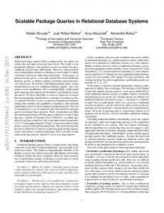
query answering in database systems. The general architecture of a Personalized Database System is depicted in Figure 1 and includes several modules surrounding a traditional Content Access module. The system keeps a repository of user information (User Profiles) that is either inserted explicitly by the user or collected implicitly by monitoring user interaction with the system (Profile Creation). This profile information is integrated into an incoming request both during content selection (Query Personalization) as well as result presentation (Presentation Personalization) and thus the overall user experience is personalized. This paper concentrates on taking advantage of User Profiles for Query Personalization for conjunctive queries in the relational model. It is not concerned with how the profiles were generated or with how result presentation may be personalized, both of which are part of our future work. Contributions. The main contributions of the paper are the following: ƒ Query personalization framework. The major steps for personalization of database queries based on information stored in atomic user profiles are: (a) preference selection, where the preferences relevant to the query and most interesting to the user are derived from the user profile, and (b) preference integration, where the derived preferences are integrated logically into the original query producing a modified, personalized one, which is actually executed. We formulate the main personalization step, i.e., preference selection, as a graph computation problem and provide an efficient algorithm for it. ƒ Preference model for user profiles. User preferences are stored as degrees of interest in atomic query elements (e.g., individual selection conditions), which may be used to transform a query. The degree of interest expresses the interest of a person to include the associated condition into the qualification of a given query. Specific logic is introduced for derivation of preferences for complex query structures building on stored atomic ones. In this way, results of a query are ranked based on the estimated degree of interest in the combination of preferences they satisfy. ƒ Experimental results. The proposed mechanism has been implemented and it is discussed through a set of experiments that show its potential. To the best of our knowledge, this work represents the first solution towards smooth integration of personalization and database queries with the use of structured user profiles. Outline. The rest of the paper is organized as follows: Section 2 presents related work. Section 3 describes the preference model for user profiles. Section 4 establishes the query personalization framework. Sections 5 and 6 describe the preference selection and preference integration steps of personalization, respectively. Section 7 presents results of experimentation with a prototype system.

Proceedings of the 20th International Conference on Data Engineering (ICDE’04) 1063-6382/04 $ 20.00 © 2004 IEEE

Finally, Section 8 presents ongoing and future work and conclusions.

Figure 1. A Personalized Database System

2. Related Work We will discuss related work using the following axes: content selection approaches, user profiles, user preferences and ranking of results. Content selection approaches can be broadly classified into three main categories. (a) Query-based approaches. Content selection is performed on the basis of a query issued. Traditional Database and IR systems fall in this category as well as two recent lines of database research inspired from IR, namely keyword searches [2, 3, 10, 11] and best-match query answering [1, 7, 12, 14, 4]. (b) Filter-based approaches. Content selection is driven by a long-term information need stored in a user profile, which is considered as a form of a continuously executing query [18, 5, 15]. (c) Personalized approaches. Content selection is based on a combination of a user query and preferences stored in a profile. The role of user profiles is twofold: they are used to focus searches and to rank results returned. Few IR systems [17] use them for both purposes simultaneously. Most of them [19] perform only result ranking. Database systems [8] focus on the construction of personal web views over database views using rules for embedding user data and propagating changes. In this paper, we propose a personalization framework for database queries based on user preferences stored in profiles. We use these to focus searches and to rank results. Preferences are dynamically extracted from a profile and incorporated into a user request. Results are ranked based on the preferences they satisfy. The whole process is independent of any changes taking place in the profiles. As far as we know, this approach is absent from the field of databases. User profiles have been broadly used for information retrieval and filtering [17, 18, 19] of text-based data items and they typically represent user preferences in terms of a single or multiple keyword vectors. User profiles have also been used for providing data management hints for preloading and pre-staging caches in distributed environments

[6, 16]. In this paper, we store user preferences in terms of atomic query constructs in profiles and we use them for individualizing user requests. User preferences provided either as query criteria or stored in profiles are of various types [7]: unconditional, conditional, multi-value etc. They are expressed as (a) hard constraints, that are either satisfied or not satisfied at all; or (b) soft constraints, that should be fulfilled as closely as possible [1, 12, 4]. Traditional SQL treats preferences as hard constraints. Soft preferences may be associated with a number indicating user satisfaction depending on how close a value is to the preferred one. Preferences on numerical data can be expressed as soft constraints (e.g., price near $20), while preferences on categorical data can be expressed as hard constraints (e.g., I prefer W. Allen). In this paper, we are concerned with unconditional, single-value preferences expressed as hard constraints. Each preference is associated to a number, which, in our case, indicates the user interest in results that exactly satisfy this preference. Moreover, we build on the database structure to derive implicit preferences, i.e., preferences not stored in the profile but inferred from the associations of objects in the database. Incorporating other types of preferences within our framework is part of ongoing work. Ranking of results is performed in several approaches: results are ordered based on the number of joins they involve [2, 3, 11] or based on how closely they match user preferences [1, 12]. In this paper, we provide a mechanism for estimating the degree of interest in a combination of preferences and we rank results returned by a personalized query, based on the combined degree of interest of the preferences they satisfy. For instance, if a user prefers actor W. Allen to R. Atkinson, a query that considers both of these preferences would return first results satisfying both, followed by these satisfying the top preference and then, those matching the second one.

3. User Preference Model Without loss of generality, we focus on SPJ (SelectProject-Join) queries over relational databases. In particular, we focus on queries, whose qualification is a combination of disjunctions and conjunctions of atomic selection and join conditions, producing a result from atomic projections of attributes. Given our focus on personalization of queries, our preference model assigns preferences to query constructs, which may then be used to transform, i.e., personalize, a given query. For instance, Julie’s interest in director W. Allen is expressed as a preference for the condition: DIRECTOR.name=‘W. Allen’

Furthermore, as entities are mutually related, preferences on one imply preferences on the other. For example, if Julie is interested in director W. Allen, then she also

Proceedings of the 20th International Conference on Data Engineering (ICDE’04) 1063-6382/04 $ 20.00 © 2004 IEEE

likes movies directed by him, expressed as a preference for the condition: MOVIE.mid=DIRECTED.mid and DIRECTED.did=DIRECTOR.did and DIRECTOR.name=‘W. Allen’

Note how the particular database schema affects preferences, in the sense that the condition associated with a desired preference is expressed through joins dictated by the schema. Finally, in a similar fashion, preferences may be expressed on arbitrary logical combinations of conditions, e.g., comedies directed by W. Allen. In the following subsections, we provide a formal description of the preference model illustrated above, starting from the simplest of conditions and building up. 3.1. Stored Atomic User Preferences Our approach to personalization is based on maintaining, for every user, a user profile whose structure is intimately related to the features of the data and query models. In particular, we assume that user preferences are stored at the level of atomic elements of queries, i.e., atomic selection or join conditions, which are therefore called atomic user preferences. A user's interest in an atomic query element is expressed in the form of a degree of interest, which is a real number in the range [0, 1]. Value 0 indicates lack of any interest in the atomic condition from the user part, while value 1 indicates extreme (‘must-have’) interest. In practice, zero-valued preferences are not stored in a user profile. The degree of interest associated with an atomic condition expresses the interest of the user to include the condition into the qualification of a given query (if appropriate) to further restrict (or sometimes expand) the universe of data that generates the query result. For the sake of simplicity in our examples, we concentrate only on equality selections and joins. A particular user’s preferences over the contents of a database can be expressed on top of the personalization graph of the database. This is a directed graph G(V, E) (V is the set of nodes and E is the set of edges) that is an extension of the traditional schema graph. There are three types of nodes in V: ƒ relation nodes, one for each relation in the schema ƒ attribute nodes, one for each attribute of each relation in the schema ƒ value nodes, potentially one for each possible value of each attribute of each relation in the schema. In essence, only those that have any interest to a particular user need to be specified Likewise, there are two types of edges in E: ƒ selection edges, from an attribute node to a value node; such an edge represents the potential selection condition connecting the corresponding attribute and value ƒ join edges, from an attribute node to another attribute node; such an edge represents the potential join condi-

tion between the corresponding attributes. These could be joins that arise naturally due to foreign key constraints, but could also be other joins that are meaningful to the designer. Finally, for reasons that will become clear later, two attribute nodes could be connected through two different join edges, in the two possible directions Moreover, given the one-to-one mapping between edges in the personalization graph and atomic query elements, it is natural to indicate degrees of interest as labels on the graph's edges. Example. Julie prefers theatres located downtown. She is a fan of comedies, enjoys thrillers, and likes adventures to a lesser extent. As far as directors are concerned, her favourite is D. Lynch followed by W. Allen. With respect to actors, she likes N. Kidman followed by A. Hopkins and I. Rossellini. These preferences are expressed as degrees of interest in specific atomic selections. Moreover, she has preferences expressed over the joins between the relations of the schema, to allow queries on one to take into account her preferences on the others. For example, she considers the director of a movie more important than the cast. All of Julie’s preferences are stored in her profile, part of which is given in Figure 2. Her profile is also depicted graphically in the personalization graph of Figure 3. [ [ [ [ [ [ [ [

THEATRE.tid=PLAY.tid, PLAY.tid=THEATRE.tid, PLAY.mid=MOVIE.mid, MOVIE.mid=PLAY.mid, MOVIE.mid=GENRE.mid, ACTOR.name=‘A. Hopkins’, GENRE.genre=‘comedy’, GENRE.genre=‘thriller’,

1 ] 1 ] 1 ] 0.8 0.9 0.8 0.9 0.7

] ] ] ] ]

Figure 2. Part of a user profile

Figure 3. A personalization graph The level of a user's desire to include a join into a query qualification may be different depending on which relation of the join is already there. For this reason, a join condition may be associated with two different degrees of interest. For example, when Julie inquires about theatres, she considers information on movies more significant than the other way around. Thus, two distinct entries (rows 3 and 4)

Proceedings of the 20th International Conference on Data Engineering (ICDE’04) 1063-6382/04 $ 20.00 © 2004 IEEE

for the same join between relations MOVIE and PLAY but with different degrees are stored in her profile as shown in Figure 2. The left part of a join of the profile corresponds to the relation already included in the query qualification. This is indicated in the personalization graph with two distinct edges with different labels corresponding to this condition, one for each possible direction from the node already included in the query to the one that is not. Preferences may evolve through time. Thus, Figure 2 and Figure 3 illustrates an instance of Julie’ profile for a given point in time. The query personalization process is not affected by changes in the profiles, since it automatically integrates recorded preferences in user requests. 3.2. Implicit/Transitive User Preferences By composing atomic user preferences that are adjacent in the personalization graph (hence, composable), one is able to build transitive user preferences, i.e., preferences expressed through relationships. Given the one-to-one mapping between edges in the personalization graph and atomic query elements, a transitive user preference is mapped to a directed path in the personalization graph. In analogy to atomic user preferences (atomic selections and joins), we consider the following types of transitive preferences: ƒ Transitive Join is mapped to a path in the personalization graph between two attribute nodes. The path is comprised of composable atomic join edges and represents the potential “implicit” join condition between the corresponding attributes. ƒ Transitive Selection is mapped to a path in the personalization graph from an attribute node to a value node. Such a path is comprised of n-1 atomic join edges and one selection edge and represents the potential “implicit” selection condition connecting the corresponding attribute and value. That is, a transitive selection is the combination of a transitive join and an atomic selection that are composable. A transitive query element is defined as the conjunction of the constituent atomic ones. In analogy to atomic user preferences, the degree of interest associated with a transitive preference expresses the interest of the user to include the corresponding transitive query element into a given query, if appropriate. Moreover, the degree of interest in a transitive preference should be a function of the degrees of interest in the participating atomic preferences. In principle, one may imagine several such functions. Any one of them, however, should satisfy the condition below, in order to be intuitive. Transitive Preference. Consider a set PN of N composable atomic preferences and the set DN of corresponding degrees of interest: DN = {di | di: degree of interest in PiPN, i = 1… N}. For any function f… calculating the degree of interest in

a transitive preference formed by the atomic preferences in PN, the following must hold: f…(DN) ” min(DN). In other words, the degree of interest in a transitive preference decreases as the length of the corresponding directed path increases, capturing human intuition and cognitive evidence [9]. Thus, we have decided to choose multiplication as the function f…: f…(DN) = d1d2 … dN. This transitive preference function essentially approaches 0 as more and more preferences are added to the combination. Example. Julie likes the actress N. Kidman, which is expressed as a preference for the selection ACTOR. name=‘N. Kidman’ with a degree of interest equal to 0.9. Then, she also likes movies starring the same actress, expressed as an implicit preference for the condition: MOVIE.mid=CAST.mid and CAST.aid=ACTOR.aid and ACTOR.name=‘N. Kidman’

The degree of interest associated with the corresponding transitive preference is the product of the degrees of the constituent conditions, which based on her profile, gives 0.8*1*0.9=0.72. Note that any directed path in the personalization graph could map to a transitive preference. However, based on human intuition and cognitive evidence [9], we deal with acyclic paths only. It is rather unlikely and unnatural that a cyclic directed path would express a confirmed user preference. Moreover, cycles have termination problems. 3.3. Logical Combination of User Preferences Given a set of user preferences, whether atomic or transitive, one may form logical combinations of them, through the Boolean operators ‘and’ and ‘or’. These result in complex conjunctive and disjunctive preferences, respectively, with the natural corresponding semantics. Again, as with transitive preferences, the degree of interest in complex preferences should be a function of the degrees of interest in the participating preferences. In principle, one may imagine several such functions for either conjunctive or disjunctive preferences, the appropriateness of each one being judged only by the philosophy of the approach taken towards personalization. Nevertheless, there are certain conditions that these functions should satisfy to be intuitive. These are stated below. Consider a set PN of N preferences (atomic or transitive) and the set DN of corresponding degrees of interest: DN = {di | di: degree of interest in PiPN, i = 1… N}. Conjunctive Preference. For any function fš calculating the degree of interest in the conjunction of the preferences in PN, the following must hold: fš (DN) • max(DN).

Proceedings of the 20th International Conference on Data Engineering (ICDE’04) 1063-6382/04 $ 20.00 © 2004 IEEE

In other words, the degree of interest in multiple preferences satisfied together increases with the number of these preferences. Disjunctive Preference. For any function f› calculating the degree of interest in the disjunction of the preferences in PN, the following must hold: min(DN) ” f› (DN) ” max(DN). That is, the degree of interest in satisfying one of several preferences is between the highest and the lowest degree of interest among the original preferences. In our approach, we have decided to choose functions fš and f› that place equal weight on each member of DN maintaining some smoothness properties as more degrees of interest are inserted in it. In particular, we have chosen the following functions: fš (DN) = 1 – (1-d1) (1-d2) … (1-dN), f› (DN) = (d1 + d2 + … + dN)/N. The conjunctive preference function essentially approaches 1 as more and more preferences are added to the combination, each participating degree of interest reducing the overall difference from 1 by a factor that is equal to its own difference from 1. The disjunctive preference function is just the average of the participating degrees of interest. Clearly, each function satisfies the corresponding condition mentioned above and both treat the degrees of interest in their input in a balanced way, as desired. Example. Consider the following transitive selections, expressing interest in movies directed by W. Allen and comedies, respectively: MOVIE.mid=DIRECTED.mid and DIRECTED.did=DIRECTOR.did and DIRECTOR.name=‘W. Allen’ MOVIE.mid=GENRE.mid and GENRE.genre=‘comedy’

Based on Julie’s profile, the degree of interest in comedies directed by W. Allen, i.e., in the conjunction of the above conditions is equal to 1-(1-1*1*0.7)(10.9*0.9)=0.943. On the other hand, her degree of interest in going to either a comedy or a W. Allen movie, i.e., in the disjunction of the above, is equal to (0.7+0.81)/2=0.755. Although there is no formal justification that functions fš and f› are appropriate for their role, the following theorem provides some strong indication. Recall that PN is a set of N (atomic and transitive) preferences and DN the corresponding set of degrees of interest. Without loss of generality, further assume that di • di+1 (1 ” i < N). Theorem: Let ƺ be the set of all conditions that represent logical combinations of preferences in PN according to the personalization model, i.e., expressing satisfaction of any L of the K most interesting preferences of PN, (L ” K ” N). For any ǚ1, ǚ2 in ƺ with degrees of interest d1 and d2, if ǚ1 is subsumed by ǚ2 for all databases, i.e., result(ǚ1) Ž result(ǚ2), then d1 • d2.

This theorem captures the intuition that strictly smaller query answers are of strictly higher interest to the user, thus indirectly providing justification for the appropriateness of the particular choices of fš and f›. Its proof is relatively tedious and is omitted due to lack of space. It takes advantage of the earlier work on conjunctive query containment and properties of fš and f›. Having established a preference model for user profiles, we now turn to describing how it can be used for query personalization.

Execution of a personalized query returns a ranked list of results, where most interesting results (based on their estimated degree of interest) come first followed by results that are less interesting to the user. Example. We will consider the initial request about movies given in the motivating example. We assume that Julie has specified that at least L = 2 of her top K = 3 preferences should be satisfied by the results; thus M = 0. We will see how the initial query can be personalized by the proposed framework given Julie’s profile.

4. Query Personalization Framework

5. Preference Selection

Query personalization is the process of enhancing a query with user-specific preferences stored in a profile. Given a query Q and a user profile U, a personalized query is built with the use of the following parameters: ƒ the number K of top preferences derived from the user profile that should affect the query ƒ the number M (0 d M d K) of top preferences from the set of the selected K ones that should be considered as mandatory, i.e. that should be definitely satisfied by all generated results ƒ the number L (L d K - M) of the remaining K - M preferences that should at least be met by the results Parameters K, M, and L can be specified with the use of various criteria. For example, a criterion for K could be that the top five preferences should affect the user request. A criterion for M could be that preferences with a degree of interest equal to 1 are considered mandatory. A criterion for L could be that at least two of the K - M preferences should be satisfied as well. These criteria may be provided at query time by the user or retrieved from the user profile based on information collected by the system. Alternatively, they may be automatically derived at query time considering various aspects that comprise the context of a query. These include desired response time, available bandwidth, etc. For instance, if the user sends a request using her mobile phone, then the system may decide to consider a few top preferences; when the user switches to her computer, then the system may decide to consider all her preferences. Analysis of aspects comprising the query context is out of the scope of this paper. Given a query Q, a user profile U and criteria for the specification of parameters K, M, and L, query personalization proceeds in two phases: (a) Preference Selection is the identification and extraction of the set of top K preferences recorded in the user profile that are relevant to the given query. (b) Preference Integration is the integration of the K selected preferences into the query in order to produce a personalized one that will return results satisfying M of them and any L of the remaining ones.

The first step of the personalization process deals with the extraction of the set PK of top K preferences from the user profile. A preference is extracted provided that it has the following properties: Property 1: It is related to the query. Property 2: It is not conflicting with the query. A preference may be related to or conflicting with a query at two different levels. Semantic level. In order to decide whether a preference is related to or conflicting with a query at this level, additional knowledge about the data is needed other than information derived from the data schema. For instance, a preference for W. Allen is semantically related to a query about comedies. On the other hand, a preference for M. Tarkowski is semantically conflicting with the same query, and, if conjunctively combined with it, no results will be returned.

Proceedings of the 20th International Conference on Data Engineering (ICDE’04) 1063-6382/04 $ 20.00 © 2004 IEEE

Figure 4. A query on top of a personalization graph Syntactic level. A preference is related to or conflicting with a query at this level, according to information provided by the data schema, as described below. ƒ Syntactically related preferences A query can be represented as a sub-graph on top of the personalization graph. This sub-graph includes all the nodes corresponding to relations that participate in the query (possibly replicated if multiple tuple variables range over them) and all the selection and join edges

corresponding to the atomic conditions of the query qualification. In all but the most artificial queries, this query graph should be connected. In addition, user preferences map to directed paths in the personalization graph. Thus a preference is syntactically related to a query, if it maps to a path that is attached to the query graph, specifically to a node involved in it, and expands outwards (i.e., it does not traverse this graph). In Figure 4, Julie’s initial query is depicted as a graph in grey colour on top of the personalization graph corresponding to her profile. An example of a (transitive) preference syntactically related to this query is this one. MOVIE.mid=GENRE.mid and GENRE.genre=‘comedy’

Preferences that are semantically related to a query are also syntactically related to it. The inverse is not generally true. ƒ Syntactically conflicting preferences A preference is conflicting with a query, if it is conflicting with a condition already there. Two conditions are syntactically conflicting, if they are comprised of a common transitive join and atomic selection conditions on the same attribute of a table and all constituent atomic joins, in the direction of the selection, are toone. For example, assume a query containing the condition theatre.region=‘uptown’; then the preference theatre.region=‘downtown’ cannot be included in the query, since a theatre can only be at one place. In the most general case, a preference may be conflicting with a query due to the existence of more than one condition. To illustrate this, consider a query that contains the conjunction of these conditions: THEATRE.tid=PLAY.tid and PLAY.mid=MOVIE.mid and MOVIE.title=‘The Last Dictator’ THEATRE.tid=PLAY.tid and PLAY.mid=MOVIE.mid and MOVIE.title=‘The Last Mohican’

In addition, consider the condition: THEATRE.tid=PLAY.tid and PLAY.date=‘2/7/2003’

Although the latter is not conflicting with each query condition individually, the conjunction of the three returns no results, since the given schema indicates that a theatre can play one movie at a time. We provide an algorithm for preference selection that is independent of the level at which conditions are considered related to or conflicting with a query. In the prototype system we have implemented, we deal with related and conflicting preferences at the syntactic level and we handle pair-wise conflicts. 5.1. Problem Formulation The problem of preference selection is formulated as a graph computation problem as described below. The preference selection problem. Consider the personalization graph GP corresponding to a user profile, a query Q represented as a sub-graph on top of this graph,

Proceedings of the 20th International Conference on Data Engineering (ICDE’04) 1063-6382/04 $ 20.00 © 2004 IEEE

and a criterion CI, referred to as interest criterion, that is used for the specification of the top K preferences to be selected. We consider the set PN of all paths Pi in GP that are related to but not conflicting with Q in decreasing order of their degree of interest, i.e.: PN = {Pi | i  [1, N], di-1 t di }. Then, the set of K preferences that must be selected based on the given interest criterion, is the ordered subset PK = {Pi | i  [1, K], di-1 t di } of PN such that: K = max({ t | t [1, N]: CI(Pt) holds }). Possible expressions of CI(.) are given in Table 1. Table 1. Expressions for interest criteria Expression t”r dt > d

Description selects at most r preferences selects preferences with degree of interest greater than d selects preferences whose disjunction has a degree of interest greater than d

· § t ¨¨ ¦ d i ¸¸ t ! d 1 i ¹ © selects preferences whose conjunction · § t 1  ¨¨ – (1  d i ) ¸¸ ! d has a degree of interest greater than d ¹ ©i 1

5.2. Preference Selection Algorithm The Preference Selection algorithm takes as input a user query Q, a user profile U and an interest criterion CI. It generates a set of preferences PK derived from the user profile, that are related to but not conflicting with the query and whose number K is decided with the help of the criterion CI. The algorithm, presented in Figure 5, is based on a best-first traversal of the personalization graph Gp that corresponds to the profile U. The basic idea is to gradually construct directed paths in decreasing order of their degrees of interest, which begin from the query graph and expand outwards. In this way, all preferences that are syntactically related to Q, are derived from the user profile in decreasing order of their degrees of interest. If we are interested in semantic related preferences, then the algorithm may output only these, since they comprise a subset of the set of syntactically related ones. Thus the algorithm does not depend on the assumptions regarding related or conflicting preferences. Preferences that are conflicting with Q are discarded. When a path that corresponds to a selection is constructed, it is output, provided that it satisfies the interest criterion. The algorithm stops when no other preferences that satisfy the interest criterion can be derived from the profile. More specifically, a queue QP of candidate preferences is kept in order of decreasing degree of interest. Initially, it contains all atomic query elements that are syntactically related to and not in conflict with the query. In each round, the algorithm picks from QP the candidate preference P with the highest degree of interest. Depending on the type

of the preference, we distinguish two cases: ƒ P is a selection: If CI(PK ‰ {P}) holds and P is related to Q, then it is added to the set PK; If CI(PK ‰ {P}) does not hold, then the algorithm terminates. ƒ P is a join: If CI(PK ‰ {P}) holds, then P is expanded into longer paths which are placed into QP; otherwise the algorithm terminates. A path P is expanded according to the following rule: a new path P š ACi is generated for each atomic element ACi that is composable with P (i.e. adjacent to P in the personalization graph). Thus each P š ACi is syntactically related to Q. Query elements ACis are considered in order of decreasing degree of interest. This helps pruning, as explained shortly, and it improves the time of insertion of new paths in the ordered QP. The new candidate is added to QP unless pruning takes place. A path P š ACi is pruned under the following circumstances: (i) it expands to a relation already existent in P, or to a relation belonging to the query Q, in which case a cycle is generated; (ii) it is conflicting with the query Q; (iii) it is not semantically related to Q (if we are interested only in them); (iv) it does not satisfy the interest criterion. In the latter case, the algorithm stops expansion of P, since all paths generated from the remaining (not yet examined ACis) are guaranteed not to satisfy the criterion, since they are considered in order of decreasing degree of interest. Paths in QP are always in order of decreasing degree of interest. When a new path is added, it should be placed after the last path with degree greater than or equal to its degree, in order to favour the selection of preferences that correspond to shorter paths among those with the same degree of interest. Subsequently, we will show that the algorithm is complete, i.e. it generates the desired set PK as defined in the previous subsection. Theorem 1: The algorithm processes preferences that are (syntactically) related to query Q in decreasing order of degree of interest. Proof: The algorithm keeps an ordered queue QP of paths. In each round, the head P of the queue (which has the greatest degree of interest) is picked and processed. Assume that P is a selection condition with degree of interest d and CI(PK ‰ {P}) holds. Then, it will be inserted into PK. In order to prove the theorem, we will show that: (a) d is greater than (or equal to) the degree of interest of any other selection in QP, and (b) d is greater than (or equal to) the degree of interest of any other selection that will be generated by successive expansions of the preferences in QP. Since QP is ordered (a) holds. In addition, for each join condition Pj  QP with degree of interest dj, it holds that d>dj. If Pj is expanded to Pj š AC and AC has a degree of interest da then: 1 t da Ÿ dj t djda. Combining the two relations, it follows that d t djda. It is clear that any selec-

Proceedings of the 20th International Conference on Data Engineering (ICDE’04) 1063-6382/04 $ 20.00 © 2004 IEEE

tion that will be generated by successive expansions of the preferences already in QP, will have a lower degree of interest than d. Consequently (b) holds.„ Based on the above theorem, the algorithm stops inspection of preferences in QP, when it encounters one that does not satisfy the interest criterion, since it is guaranteed that the remaining ones have lower degrees of interest. Furthermore, when the algorithm picks a join condition that does not meet the criterion, it stops on the ground that all preferences that will be generated by extending this join (and any subsequent join) shall not meet the criterion. Consequently, theorem 2 follows. Theorem 2 (Completeness): The algorithm is complete i.e., it generates the set PK that contain all related preferences according to an interest criterion. Example. Returning to our example, after completion of the preference selection step, the personalization system has extracted the following selections from Julie’s profile: MOVIE.mid=GENRE.mid and GENRE.genre=‘comedy’, MOVIE.mid=DIRECTED.mid and DIRECTED.did=DIRECTOR.did and DIRECTOR.name=‘D. Lynch’, MOVIE.mid=CAST.mid and CAST.aid=ACTOR.aid and ACTOR.name=‘N. Kidman’

Preference Selection Algorithm Input: User profile U User query Q Interest Criterion CI Output: Set of selections PK

PK ={}, QP={} 1. Foreach atomic element ACiU syntactically related to Q 1.1 If (ACi is conflicting with Q) Then discard ACi

Else QP Å ACi End if End for 2. While (QP not empty) 2.1 Get head P from QP 2.2 If (P is selection) Then If (CI(PK ‰ {P})=TRUE) Then PK ÅP Else Stop End if End if 2.3 If (P is join) Then If (CIS(PK ‰ {P})=TRUE) Then Foreach atomic element ACiU composable with P If (CI(PK ‰ {P š ACi})=FALSE) Then Exit For End if If Not ((ACi joins to relation RP or RQ) or (PšACi is conflicting with Q)) and (P is related to Q) Then QPÅP š ACi End if End for Else Stop End if End if End while 3. Output PK

Figure 5. Preference Selection Algorithm

6. Preference Integration The purpose of this step is to integrate the K selected preferences into the original query and produce a new, personalized query that will generate satisfactory results for the user, i.e., those satisfying the M top preferences of those and at least L preferences from the remaining K - M ones. Towards this direction, we consider the set of K preferences derived from the profile, in order of decreasing degree of interest. We consider the first M conditions of this set as mandatory. M is an integer in the range [0, K] and it is specified (explicitly or implicitly) with the help of a criterion, whose expression may be one of those used for interest criteria. For example, such a criterion may specify that preferences with a degree of interest equal to 1 are considered mandatory. In addition, the number L, which is an integer in the range [0, K - M], may be specified either explicitly or implicitly by specifying the minimum degree of interest d for every row in the results (each row may satisfy one or more preferences). Given the parameters M and L, the personalized query can be constructed following two different (but equivalent) approaches. The most straightforward way is to build a single complex qualification that is a conjunction of: ƒ The conjunction of the mandatory conditions, and ƒ The disjunction of all possible conjunctions of L conditions from the remaining K - M ones. The qualification is embedded into the original query and any repeated conditions are removed. Furthermore, any additional tuple variables required for the preference conditions are also incorporated into the query. We refer to this approach as SQ (Single Query). Example. Returning to our example, Julie’s initial request is transformed into the following personalized query: select distinct MV.title from MOVIE MV, PLAY PL, CAST CA, ACTOR AC, GENRE GN, DIRECTED DD, DIRECTOR DI where MV.mid=PL.mid and PL.date=‘2/7/2003’ and ( ((MV.mid=GN.mid and GN.genre=‘comedy’ and MV.mid=CA.mid and CA.aid=AC.aid and AC.name=‘N. Kidman’)) or ((MV.mid=CA.mid and CA.aid=AC.aid and AC.name=‘N. Kidman’ and MV.mid=DD.mid and DD.did=DI.did and DI.name=‘D. Lynch’)) or ((MV.mid=GN.mid and GN.genre=‘comedy’ and MV.mid=DD.mid and DD.did=DI.did and DI.name=‘D. Lynch’)))

The second approach is to formulate a set of K - M queries, each one containing a simpler qualification, which is a conjunction of the mandatory conditions, and one condition from the remaining K - M ones. Each of these queries

Proceedings of the 20th International Conference on Data Engineering (ICDE’04) 1063-6382/04 $ 20.00 © 2004 IEEE

is built around the initial query extending it with the corresponding qualification and the set of new tuple variables used in the latter. The expected results are obtained by taking the union of the partial results, grouping by the projected attributes of the initial query, and excluding all groups containing less than L rows. We refer to this approach as MQ (Multiple Queries). Example. Following this approach, Julie’s initial request is transformed into the following personalized query: select from

MV.title ((select distinct MV.title from MOVIE MV, PLAY PL, MGENRE GN where MV.mid=PL.mid and PL.date=‘2/7/2003’ and MV.mid=GN.mid and GN.genre=‘comedy’) Union All ( select distinct MV.title from MOVIE MV, PLAY PL, CAST CA, ACTOR AC where MV.mid=PL.mid and PL.date=‘2/7/2003’ and MV.mid=CA.mid and CA.aid=AC.aid and AC.name=‘N. Kidman’) Union All ( select distinct MV.title from MOVIE MV, PLAY PL, DIRECTED DD, DIRECTOR DI where MV.mid=PL.mid and PL.date=‘2/7/2003’ and MV.mid=DD.mid and DD.did=DI.did and DD.name=‘D. Lynch’)) TEMP group by MV.title having count(*) >= 2

The MQ approach has some obvious advantages compared to the first one. Provided that each partial query returns results accompanied with their degree of interest, the following options are possible: ƒ L may also be specified implicitly by providing a desired minimum degree of interest d in every row in the results. Using the MQ approach, it is easy to build a query that returns results that have an estimated degree of interest greater than d. The only modification required is the replacement of the having part of the query with this one: having DEGREE_OF_CONJUNCTION(*) > d

where DEGREE_OF_CONJUNCTION is an aggregate function that calculates the degree of interest in a row returned that satisfies a conjunction of preferences, i.e., is returned by a set of partial queries. ƒ It is easy to rank results based on their estimated degree of interest. The afore-mentioned aggregate function is included into the select part of the query and results are ordered based on the values returned by this function using an appropriate order by clause. An apparent drawback of MQ compared to SQ seems to be the repetitive execution of the mandatory part of the query. We have implemented and evaluated both approaches.

MOVIE.mid=CAST.mid and CAST.role=‘Batman’ MOVIE.mid=cast.mid and CAST.aid=ACTOR.aid and ACTOR.name=‘A. Hopkins’

Their conjunction using the same tuple variables qualifies films in which A. Hopkins played the role of Batman. Furthermore, if common variables are used, preferences on the same attribute that are not conflicting are forced to be treated as “one” condition. Consider the following preferences: MOVIE.mid=CAST.mid and CAST.aid=ACTOR.aid and ACTOR.name=‘I. Rossellini’ MOVIE.mid=CAST.mid and CAST.aid=ACTOR.aid and ACTOR.name=‘A. Hopkins’

If common tuple variables are used, a conjunction that

Proceedings of the 20th International Conference on Data Engineering (ICDE’04) 1063-6382/04 $ 20.00 © 2004 IEEE

explicitly qualifies movies that both actors star is excluded from the qualification of the desired results. Based on the above observations, when a choice is possible, different tuple variables should be used and this action should be performed as close as possible to the start of the paths (i.e. at the first to-many common atomic join of these paths).

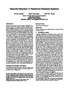
7. Experimental Results In order to evaluate the proposed framework, we have implemented a prototype system on top of Oracle 9i. In this section, we present results of our experiments. Our data primarily comes from the Internet Movies Database [13]. The schema described in the motivating example represents part of the actual database created for the experiments, which contains information about over 340000 movies. User profiles are stored in a separate table. For the experiments we have used both synthetic and real user profiles. The former were automatically produced with the use of a profile generator. Real profiles were populated by individuals. We ran four different sets of experiments. In all these experiments, we used a set of 100 randomly created queries and we considered the number of mandatory preferences M equal to zero. (All times are shown in milliseconds). Effect of Profile Size on Preference Selection Time. In this set of experiments, we measured the execution time of the preference selection algorithm (Preference Selection Time) for varying profile sizes. We consider the number of atomic selections in a profile as the profile size. For each different value of it, we used 100 profiles of that size. We measured the Preference Selection Time for each query and profile combination, for L=1. We ran the experiments three times, using a different number of preferences (K=5, 10, 15). Figure 6 summarizes our results. In this figure, we have calculated the average Preference Selection Time, grouped by the profile size for different values of K. Preference Selection Time with Profile Size 0,06 Preference Selection Time

Independent of the preference integration method used (SQ vs. MQ), construction of conjunctions of conditions is not straightforward. Two issues must be considered: (a) Conflicting conditions As already mentioned in a previous section, conflicting conditions cannot be concurrently satisfied, i.e., combined into a conjunction. Therefore, they can only be combined using disjunction, and they are essentially treated as “one” condition. This has the same effect to excluding from the qualification of a query all conjunctions that contain conflicting conditions, and results in a reduction of the size of the SQL query that must be parsed and executed with obvious benefits. In the current implementation, we deal with syntactically conflicting conditions as defined in section 5. (b) Common tuple variables Conditions may share common relations (apart from those belonging to the original query). This fact gives rise to the question of whether common or different tuple variables should be used, when building conjunctions of the former. This may occur in the following cases. Case 1: Conditions map to paths that traverse different sets of nodes on the personalization graph till they meet at a node (relation). The same or different tuple variables may be possibly used for this relation. Case 2: Conditions share a common initial transitive join followed by atomic selections or different transitive joins. In the latter case, if common atomic joins are to-one in the direction of the selection, then using common tuple variables for all common relations is the only option. If these conditions are conflicting, then the use of disjunction is mandatory. On the other hand, if there is a common atomic join in the direction of the selection that is tomany, it is possible to use different tuple variables at this point. If more than one such joins exist, then the decision may be taken in any of these points. In both cases 1 and 2, the use of common tuple variables imposes an additional constraint that all conditions should be met by the same object. However, such a constraint is not expressed in the preference model, which assumes single, independent preferences. For instance, consider the following preferences:

0,05 0,04

K=5

0,03

K=10 K=15

0,02 0,01 0 10

20

30

40

50

60

70

80

90

100

Profile Size

Figure 6. Pref. Selection Time with Profile Size We show that, when the size of the profile is smaller, Preference Selection Time is longer. This is primarily due to the fact that, in small profiles, there is a greater probability that preferences are sparsely placed over the schema graph, resulting in more database accesses.

Size of the Results of personalized queries. In this set of experiments, we measured the change in the size of the results obtained from the personalized queries compared to those obtained from the original ones. We chose 200 random user profiles and ran the personalization algorithm for several different values of K and L parameters. In each run, we calculated the percentage of rows returned by the personalized query to those returned by the initial one.

paper, have shown that if a small query is built, then the execution time of the personalized query is significantly reduced and overall performance of the method is improved. Nevertheless, MQ execution times are better. This is explained by the fact that as more preferences come into the query, each result is returned more times by SQ (due to the existence of many joins and the semantics of SQL) and then the duplicates need to be eliminated. Preference Integration Times with K

80

Preference Integration Time

% of Rows of the Initial Query

Size of the Results of Personalized Queries with K 90 70 60 50 40 30 20 10 0 10

20

30

40

0,035 0,03 0,025 0,02

0,01 0,005 0

50

0

Number of Preferences K

(a)

SQ MQ

0,015

5

10

20

30

40

50

60

Number of Preferences K

Size of the Results of Personalized Queries with L (K=10)

Execution Times with K

18 16

1,6

14

1,4

12

1,2

Execution Time

% of Rows of the Initial Query

20

10 8 6 4 2

1

SQ MQ

0,8 0,6 0,4 0,2

0 1

2

3

4

5

6

7

8

9

10

0 0

M inimum Number of Preferences L

(b)

5

10

20

30

40

50

60

Number of Preferences K

Size of the Results of Personalized Queries with L (K=60)

Figure 8. Comparison of SQ and MQ with K Figure 9 shows that, for varying L and K = 10 preference integration times using MQ are practically zero. In addition, execution times of queries constructed using MQ are better than those for SQ’s. This is due to the fact that

70 60 50 40 30 20 10 0 1

5

10

15

20

25

Minimum Number of Preferences L

(c) Figure 7. Size of results of personalized queries The results follow the trends expected by the nature of K and L: Figure 7(a) shows the increase in the relative size of the query results as K ranges between 10 and 50 and L = 1. Figures 7(b) and 7(c) show the reduction in the relative result size as L ranges between 1 and 10 and K is 10 and 60, respectively. It is interesting to observe that despite the expected difference in scales of the axes of the last two graphs, the shapes of the two curves are very similar to each other. Comparison of SQ and MQ. In this set of experiments, we compared the performance of SQ and MQ integration approaches. We chose a set of 200 random profiles and ran each preference integration method for several different values of K and L parameters. The results are presented in Figures 8 and 9. Figure 8 shows that, for varying K and L = 1, the preference integration time using MQ is practically zero. For SQ, this time increases, mostly because it spends time on trying to eliminate repeated conditions and build a minimal query. Experiments not presented in this

Proceedings of the 20th International Conference on Data Engineering (ICDE’04) 1063-6382/04 $ 20.00 © 2004 IEEE

SQ depends on the number §¨ K  M ·¸ L

©

( K  M )!

¹

of com-

L! ( K  M  L )!

binations it has to build, while MQ depends on the number

K - M of simple queries it has to construct. Preference Integration Times with L (K=10)

Preference Integration Time

80

0,006 0,005 0,004 SQ MQ

0,003 0,002 0,001 0 1

2

3

4

5

6

7

8

9

10

Minimum Number of Preferences L

Execution Times with L (K=10) 1,2 1 Execution Time

% of Rows of the Initial Query

90

0,8 SQ MQ

0,6 0,4 0,2 0 1

2

3

4

5

6

7

8

9

10

Minimum Number of Preferences L

Figure 9. Comparison of SQ and MQ with L

Performance of Personalization. In this set of experiments, we evaluated the performance of personalization. We chose a set of 200 random profiles. We have employed the MQ approach. As Figure 10 shows, the overall time for personalization of a query and execution of the personalized one is less than the time required for the execution of the initial one. Most specifically, personalization performs well with K and is independent of L. Performance of Personalization with K 0.7 0.6

Time

0.5

Initial Query Exec.Time

0.4

Personal. Query Exec.Time

0.3

Personalization Time

0.2 0.1 0 0

5

10

20

30

40

50

60

Number of Preferences K

Performance of Personalization with L (K=10) 0.7 0.6

Time

0.5

Initial Query Exec.Time

0.4

Personal. Query Exec.Time

0.3

Personalization Time

0.2 0.1 0 1

2

3

4

5

6

7

8

9

10

Minimum Number of Preferences L

Figure 10. Performance of Personalization

8. Conclusions and Future Work We have presented a personalization framework for database queries based on information stored in structured user profiles that keep single, unconditional preferences. We have formulated the main personalization step as a graph computation problem and we have presented and evaluated, through a number of experiments, algorithms for the personalization of a query. We are currently working towards extending our model in order to encompass more types of preferences, such negative and soft ones, and personalizing queries using these types. We are also interested in combining personal preferences with other aspects of a query’s context that call for query customization, such as time of day, user location, device used for querying, etc, and see what kind of statistics may be additionally needed and how they are obtained. Experiments with humans are performed to solidify the evidence on the effectiveness of the approach. We are also interested in investigating ways of optimizing personalized queries in terms of running time and result size constraints. Our future plans include the study of other ways for the efficient execution of personalized queries and the delivery of top-N results in order of the estimated of degree of interest. Other challenging issues include the identification of related and conflicting preferences at the semantic level, the evaluation of various func-

Proceedings of the 20th International Conference on Data Engineering (ICDE’04) 1063-6382/04 $ 20.00 © 2004 IEEE

tions for disjunctive and conjunctive preferences and the automatic construction of structured profiles. Finally, it is interesting to see how database technology can be extended in order to support such functionality from “within”, instead of implementing a system on top of a database management system.

References [1] R. Agrawal, E. Wimmers. A Framework for Expressing and Combining Preferences. In Proc. of ACM SIGMOD, 2000. [2] S. Agrawal, S. Chaudhuri, G. Das. DBXplorer: A System For Keyword-Based Search Over Relational Databases. In Proc. of Intl. Conf. on Data Engineering, 2002. [3] G. Bhalotia, C. Nakhey, A. Hulgeri, S. Chakrabarti, S. Sudarshan. Keyword Searching and Browsing in Databases using BANKS. In Proc. of Intl. Conf. on Data Engineering, 2002. [4] S. Chaudhuri, L. Gravano. Evaluating Top-k Selection Queries. In Proc. of the 25th Int’l Conf. On VLDB, 1999. [5] J. Chen, D. DeWitt, F. Tian, Y. Wang. NiagaraCQ: A Scalable Continuous Query System for Internet Databases. In Proc. of SIGMOD, 2000. [6] M. Cherniack, E. Galvez, M. Franklin, S. Zdonik. ProfileDriven Cache Management. In Proc. of Intl. Conf. on Data Engineering, 2003. [7] J. Chomicki. Querying with Intrinsic Preferences. In Proc. of the 8th EDBT 2002. [8] K. T. Claypool, L. Chen and E. Rundensteiner. Personal Views for Web Catalogs. Bulletin of the Technical Committee on DE, March 2000 Vol. 23 No. 1. [9] A. Collins, M. Quillian. Retrieval Time from Semantic Memory. J. of Verbal Learning and Verbal Behaviour, Vol 8, pp. 240-247, 1969. [10] D. Florescu, D. Kossmann, I. Manolescu. Integrating Keyword Search into XML Query Processing. 9th WWW Conference 2000, Computer Networks, 33(1-6): 119-135. [11] V. Hristidis, Y. Papakonstantinou. DISCOVER: Keyword Search in Relational Databases. In Proc. of the 28th Int’l Conf. On VLDB, 2002. [12] V. Hristidis, N. Koudas, Y. Papakonstantinou. PREFER: A System for the Efficient Execution of Multi-parametric Ranked Queries. In Proc. of ACM SIGMOD, 2001. [13] Internet Movies Database. Available at www.imdb.com [14] W. Kießling, G. Köstler. Preference SQL-Design, Implementation, Experiences. In Proc. of the 28th Int’l Conf. On VLDB 2002. [15] L. Liu, C. Pu, W. Tang. Continual Queries for Internet Scale Event-Driven Information Delivery. TKDE 11(4), pages 610-628, 1999. [16] F. Perich, S. Avancha, D. Chakraborty, A. Joshi, Y. Yesha. Profile driven Data Management for Pervasive Environments. DEXA 2002, LNCS 2453, pp.361 –370, 2002. [17] J. Pitkow, H. Schutze, T. Cass, R. Cooley, D. TurnBull, A. Edmonds, E. Adar, T. Breuel. Personalized Search. Communications of the ACM, Vol. 45(9) September2002. [18] C. Shahabi, F. Banaei-Kashani, Y. Chen, D. McLeod. Yoda: An Accurate and Scalable Web-based Recommendation System. In Proc. of 9th Int’l Conf. On COOPIS, 2001. [19] B. Smyth, K. Bradley, R. Rafter. Personalization Techniques for Online Recruitment Services. Communications of the ACM Vol 45, 2002.