Perturbation and Truncation of Probability Generating Function

Hindawi Publishing Corporation Journal of Applied Mathematics Volume 2015, Article ID 864238, 8 pages http://dx.doi.org/10.1155/2015/864238

Research Article Perturbation and Truncation of Probability Generating Function Methods for Stiff Chemical Reactions Soyeong Jeong, Pilwon Kim, and Chang Hyeong Lee Department of Mathematical Sciences, School of Natural Science, Ulsan National Institute of Science and Technology (UNIST), Ulsan Metropolitan City 689-798, Republic of Korea Correspondence should be addressed to Pilwon Kim; [email protected] and Chang Hyeong Lee; [email protected] Received 15 September 2014; Revised 3 February 2015; Accepted 6 February 2015 Academic Editor: Lotfollah Najjar Copyright © 2015 Soyeong Jeong et al. This is an open access article distributed under the Creative Commons Attribution License, which permits unrestricted use, distribution, and reproduction in any medium, provided the original work is properly cited. One can reformulate chemical master equations of the stochastic reaction network into a partial differential equation (PDE) of a probability generating function (PGF). In this paper, we present two improvements in such PGF-PDE approach, based on perturbation and double-truncation, respectively. The stiff system that involves fast and slow reactions together often requires high computational cost. By applying the perturbation method to PGF-PDEs, we expand the equation in terms of a small reaction rate which is often responsible for such stiffness of the system. Also by doubly truncating, we dump relatively small terms and reduce the computational load significantly at each time step. The terms corresponding to rare events are sieved out through truncations of Taylor expansion. It is shown through numerical examples of enzyme kinetics, transition model, and Brusselator model that the suggested method is accurate and efficient for approximation of the state probabilities.

1. Introduction Stochastic chemical kinetics arises mostly in the modeling of chemical reactions in relatively small biochemicalbhlt systems such as gene regulatory networks, cell systems, and protein folding models [1]. The governing equation, chemical master equation (CME), describes the probability distribution of the system under the Markov assumption as 𝜕 𝑝 (n, 𝑡) = ∑𝑎𝑘 (n − 𝑉𝑘 ) ⋅ 𝑝 (n − 𝑉𝑘 , 𝑡) 𝜕𝑡 𝑘

(1)

− ∑𝑎𝑘 (n) ⋅ 𝑝 (n, 𝑡) , 𝑘

where n(𝑡) = (𝑛1 (𝑡), 𝑛2 (𝑡), . . . , 𝑛𝑠 (𝑡)), each 𝑛𝑖 (𝑡) denotes the molecular number of 𝑖th species at time 𝑡, 𝑎𝑘 is the propensity function or probability intensity for the 𝑘th reaction, and 𝑉𝑘 denotes the 𝑘th column of the stoichiometric matrix 𝑉 of which (𝑖, 𝑗)th entry is the change in the number of molecules of the 𝑖th species by the occurrence of the 𝑗th reaction [2]. Since (1) is a high dimensional system in most real applications, it is very challenging to handle both analytically and computationally. One of the key methods to help simplify

the computation of the stochastic dynamics is done by using the stochastic simulation algorithm (SSA) [3]. One realization of the SSA shows the trajectory of the timeevolution of the states. Since it is basically a Monte-Carlo type algorithm, one has to perform many realizations to obtain important statistical quantities such as mean and variance. Moreover, it often requires a large number of realizations, especially in cases of the systems consisting of large numbers of molecules or very different time scale reactions. There have been many approaches to improve the SSA including Tauleaping methods [4–6], reduction methods on the slow time scale [7–10], and moment closure methods [11–13]. In the recent papers [14, 15], the authors presented numerical schemes based on probability generating functions (PGF) for finding the probability distribution and moments. One can reformulate chemical master equations of the stochastic reaction network into a partial differential equation (PDE). Although such PDEs are mostly hard to deal with due to variable coefficients and lack of proper boundary conditions, several improvements in approximation of the moments based on Pade approximation and numerical superimposition have been made.

2

Journal of Applied Mathematics

In this paper, we present two improvements in such PGFPDE approach. The first method is an approximation method called “perturbed probability generating function (PPGF) method.” By applying the perturbation method to PDEs, we expand the equation in terms of a small reaction rate which is often responsible for the stiffness of the system. This enables us to handle the system more efficiently with less iteration and therefore capture same accuracy faster. We also develop the double truncation method (DTM) that efficiently approximates the state probabilities. As suggested from the name, the method combines two truncation procedures for the series solution to PGF-PDEs. Through consecutive truncations of the Taylor expansion of such PDEs in time, one can dump relatively rare events which correspond to excessive occurrence of reactions during a short time interval. This elimination is justified from the fact that the coefficient of each term in the PGF is the probability of a specific state. This enables us to ignore a great deal of small terms which do not affect the system significantly. An outline of the paper is as follows. In Section 2, we review the properties of PDEs that PGF should satisfy. The perturbation of PGF is discussed in Section 3 with its numerical accuracy of through some examples. Section 4 presents the double truncation method for the PGF-PDEs. In Sections 3 and 4, we also illustrate numerical accuracy of the method in several examples.

2. PGF-PDE Approach ∞

n

𝐺 (z, 𝑡) = ∑ z 𝑝 (n, 𝑡) ,

(2)

n=0

where z = (𝑧1 , . . . , 𝑧𝑠 ), 𝑧𝑖 ∈ [−1, 1], n = (𝑛1 , 𝑛2 , . . . , 𝑛𝑠 ), and 𝑛

zn ≡ 𝑧1 1 𝑧2 2 ⋅ ⋅ ⋅ 𝑧𝑠𝑛𝑠 .

(3)

After differentiation of (2) with respect to 𝑡 and application of (1), one can derive a PDE 𝜕𝐺 = ∑ 𝐻 (z, 𝑡) 𝐷k 𝐺. 𝜕𝑡 |k|≤𝑚 k

(4)

Here k = (𝑘1 , . . . , 𝑘𝑠 ), |k| = 𝑘1 + ⋅ ⋅ ⋅ + 𝑘𝑠 , 𝑚 is the highest order of the reactions in the chemical system, and 𝐷k 𝐺 denotes any 𝑘th order partial derivatives of 𝐺 as 𝐷k 𝐺 =

𝜕𝑘1 𝜕𝑘2 𝑘

𝐺 (z = 0, 𝑡) = 𝑝 (n = 0, 𝑡) , (7)

𝐺 (z = 1, 𝑡) = ∑𝑝 (n, 𝑡) = 1. n

Using the solution 𝐺 of the PDE (4), one can find the important information for stochastic reaction network such as marginal probability, mean, and the second moment [14]. If 𝑁𝑖 (𝑡) denotes the number of molecules of 𝑖th species at time 𝑡, the probability that 𝑁𝑖 = ℓ at time 𝑡 is 𝑝(𝑁𝑖 = ℓ, 𝑡) =

󵄨 1 𝜕ℓ 𝐺(z, 𝑡) 󵄨󵄨󵄨 󵄨󵄨 , ℓ ℓ! 𝜕𝑧𝑖 󵄨󵄨󵄨 𝑧𝑖 =0,𝑧𝑗 =1,𝑗=𝑖̸

(8)

and the mean and second moment are obtained by the first and second derivatives of 𝐺 𝜕 𝐺 (z = 1, 𝑡) = 𝐸 [𝑁𝑖 (𝑡)] , 𝜕𝑧𝑖 {𝐸 [𝑁𝑖 (𝑡) 𝑁𝑗 (𝑡)] , 𝜕2 𝐺 (z = 1, 𝑡) = { 𝜕𝑧𝑖 𝜕𝑧𝑗 (𝐸 [𝑁𝑖2 (𝑡)] − 𝐸 [𝑁𝑖 (𝑡)]) , {

if 𝑖 ≠ 𝑗, if 𝑖 = 𝑗, (9)

where 𝐸[𝑋(𝑡)] denotes the expectation of 𝑋(𝑡).

The probability generating function is defined as

𝑛

where n0 is the initial condition of n, and also it is true that

𝑘

𝜕𝑧1 1 𝜕𝑧2 2

⋅⋅⋅

𝜕𝑘𝑠 𝑘

𝜕𝑧𝑠 𝑠

𝐺.

(5)

One can see that the PDE (4) is linear and 𝐻k is a polynomial function of degree at most order 𝑚 which satisfies 𝐻k (z = 1, 𝑡) = 0 for |k| = 0, 1, . . . , 𝑚. The conditions of the PDE (4) can be found from the conditions on 𝑛 [14]. The initial condition is 𝐺 (z, 𝑡 = 0) = zn0 ,

(6)

3. Perturbation of Probability Generating Function Method 3.1. Perturbation of PGF. For the PGF method recently proposed in [14], 𝐺(z, 𝑡) is represented by a power expansion with respect to 𝑡 as ∞

𝐺 (z, 𝑡) = ∑ 𝑓𝑛 (z) 𝑡𝑛 ,

(10)

𝑛=0

where 𝑓𝑛 , 𝑛 = 0, 1, . . ., are coefficient functions of z. Note that the initial condition determines the first coefficient as 𝑓0 (z) = zn0 . Suppose that the reaction rates in the network do not change with time and therefore the coefficients of the PDE do not involve 𝑡 explicitly. This implies 𝐻k (z, 𝑡) = 𝐻k (z) in (4). Plugging (10) into the both sides of (4) and comparing the power series lead to a recursive relation between 𝑓𝑛+1 (z) and 𝑓𝑛 (z), 𝑛 = 0, 1, . . .. One can derive coefficient functions 𝑓1 (z), 𝑓2 (z), . . . , 𝑓𝐽 (z) from 𝑓1 (z) = zn0 and then construct an approximation ∑𝐽𝑛=0 𝑓𝑛 (z)𝑡𝑛 for sufficiently large 𝐽. Since the initial function 𝑓0 (z) and the coefficient of the PDE (2) are polynomials, all 𝑓𝑛 (z) generated are polynomials as well. Now, let us apply the perturbation method to PGF. Since many practical chemical networks that interest us involve reactions in a broad range of time scales, from seconds to microseconds, it is important to efficiently handle such stiffness in simulation of the systems. Suppose that 𝑐 ≪ 1 is

Journal of Applied Mathematics

3

a small reaction rate in the system; then one can expand the PGF as

After the removal, we can derive a PDE of 𝐺(𝑧1 , 𝑧2 , 𝑡) from the master equation [14]

𝐺 (z, 𝑡) = 𝑔0 (z, 𝑡) + 𝑐𝑔1 (z, 𝑡) + 𝑐2 𝑔2 (z, 𝑡) + ⋅ ⋅ ⋅ , ∞

𝐺𝑡 = 𝑐1 (1 − 𝑧1 𝑧2 ) 𝐺12 + ((𝑐−1 + 𝑐2 ) 𝑧1 − 𝑐−1 𝑧12 𝑧2 − 𝑐2 𝑧12 ) 𝐺1

(11)

= ∑𝑐𝑗 𝑔𝑗 (z, 𝑡) , 𝑗=0

(16)

+ 𝐴 (𝑐−1 𝑧1 𝑧2 + 𝑐2 𝑧1 − (𝑐−1 + 𝑐2 )) 𝐺.

where 𝑔𝑗 (z, 𝑡), 𝑗 = 0, 1, 2, . . ., are functions to be determined. As in (10), one can set for each 𝑔𝑗

Here 𝐴 is the conserved quantity 𝑛1 + 𝑛3 and we use the notations

∞

𝑔𝑗 (z, 𝑡) = ∑ 𝑓𝑗,𝑘 (z) 𝑡𝑘 .

𝐺𝑖 =

(12)

𝑘=0

Now, instead of (10), one can seek 𝐺(z, 𝑡) in the following form: ∞

∞

𝑗=0

𝑘=0

𝐺 (z, 𝑡) = ∑𝑐𝑗 ∑ 𝑓𝑗,𝑘 (z) 𝑡𝑛 𝑀

𝑗

𝐺𝑖𝑗 =

𝜕2 𝐺 , 𝜕𝑧𝑖 𝜕𝑧𝑗

𝑖, 𝑗 = 1, 2, . . . .

(17)

In the example, we use parameters 𝑐1 = 0.01𝑠−1 , 𝑐−1 = 1𝑠 , and 𝑐3 = 1𝑠−1 and let the perturbation be expanded in 𝑐1 . Figure 1 shows comparison of the exact solution of the master equation (15) and the approximate solution obtained from the PPGF method. −1

(13)

𝑁

𝑘

𝑀+1

= ∑𝑐 ∑ 𝑓𝑗,𝑘 (z) 𝑡 + 𝑂 (𝑐 𝑗=0

𝜕𝐺 , 𝜕𝑧𝑖

𝑁+1

,𝑡

3.3. Example 2: Brusselator Model. We consider the Brusselator model:

)

𝑘=0

𝑐1

for large 𝑀 and 𝑁. By plugging (13) into the both sides of (4) and comparing the power series, one can find recurrence relations for 𝑓𝑗,𝑘 , 𝑓𝑗+1,𝑘 and 𝑓𝑗+1,𝑘+1 , where 𝑗, 𝑘 = 0, 1, 2, . . .. This decomposition enables us to handle stiffness caused by 𝑐 properly, by adjusting the perturbation order 𝑀 as will be shown in the numerical examples in the next sections. 3.2. Example 1: Enzyme Kinetics. As the first application, we consider a fundamental chemical kinetic model, the enzymesubstrate reaction system 𝑐1

𝑐2

→ 𝐸 + 𝑃, 𝐸 + 𝑆 󴀘󴀯 𝐸𝑆 󳨀 𝑐−1

(14)

where 𝐸, 𝑆, 𝐸𝑆, and 𝑃 denote enzyme, substrate, enzymesubstrate complex, and product, respectively, and 𝑐1 , 𝑐−1 , and 𝑐2 are probability constants for reactions. If we denote the molecular numbers of 𝐸, 𝑆, 𝐸𝑆, and 𝑃 by 𝑛1 , 𝑛2 , 𝑛3 , and 𝑛4 , respectively, the governing equation of the stochastic enzyme-substrate system is obtained [16] as 𝜕𝑝 (𝑛1 , 𝑛2 , 𝑛3 , 𝑛4 , 𝑡) 𝜕𝑡

𝑐2

2𝑋 + 𝑌 󳨀 → 3𝑋,

𝑐3

𝐵+𝑋󳨀 → 𝑌 + 𝐷,

𝑐4

(18)

𝑋󳨀 → 𝐸.

Here 𝑋, 𝑌 are molecular species and 𝐴, 𝐵, 𝐷, and 𝐸 are constant species. The Brusselator is a generic model for a type of autocatalytic reaction. It is well known that the model reveals simple chemical oscillations. Refer to Figure 2(a) for a typical run of the model. If we denote the number of 𝑋, 𝑌 by 𝑛1 , 𝑛2 , respectively, we obtain the PDE for the probability generating function as follows: 𝐺𝑡 = 𝑐1 𝐴 (𝑧1 − 1) 𝐺 +

𝑐2 2 𝑧 (𝑧 − 𝑧2 ) 𝐺112 2 1 1

(19)

+ 𝑐3 𝐵 (𝑧2 − 𝑧1 ) 𝐺1 + 𝑐4 (1 − 𝑧1 ) 𝐺1 . Here 𝐴 = 𝐵 = 1 and the reaction rates 𝑐1 = 1𝑠−1 , 𝑐2 = 0.0001𝑠−1 , and 𝑐3 = 𝑐4 = 0.1 are used. We use PPGF with respect to the smallest parameter 𝑐2 . Figure 2 compares the corresponding numerical result to those from SSA.

4. Double Truncation Method

= 𝑐1 (𝑛1 + 1) (𝑛2 + 1) ⋅ 𝑝 (𝑛1 + 1, 𝑛2 + 1, 𝑛3 − 1, 𝑛4 , 𝑡)

→ 𝑋, 𝐴󳨀

(15)

+ 𝑐−1 (𝑛3 + 1) 𝑝 (𝑛1 − 1, 𝑛2 − 1, 𝑛3 + 1, 𝑛4 , 𝑡) + 𝑐2 (𝑛3 + 1) 𝑝 (𝑛1 − 1, 𝑛2 , 𝑛3 + 1, 𝑛4 − 1, 𝑡) − (𝑐1 𝑛1 𝑛2 + 𝑐−1 𝑛3 + 𝑐2 𝑛3 ) 𝑝 (𝑛1 , 𝑛2 , 𝑛3 , 𝑛4 , 𝑡) . One can see that there are two conservation quantities in the system and thus we can remove two of variables, say 𝑛3 , 𝑛4 .

4.1. Truncations in 𝑡 and z. The truncation method was firstly introduced in [15] to deal with PGF-PDEs. Although the method provides a fast way to evaluate the mean and the variance, most of high order terms need to be thrown away for efficient computations at each time step. As a result, the statistical information that is carried in high order terms, such as the higher order moments and the probabilities of the states, is generally not available from the method. In this section, we develop an extension of the truncation method which enables us to carry high order terms in the computation. This is done by another truncation in z at each step. Note that this is not just additional manipulation to

4

Journal of Applied Mathematics 1

5.3

0.9

+𝜎

5.1

0.8

5

0.7

4.9

0.6

Probability

E[e]

5.2

4.8 4.7 −𝜎

4.6

0.5

4.4

0.1 20

P(s = 2)

0.3 0.2

0

P(s = 1)

0.4

4.5

4.3

P(s = 0)

40

60

80

100

0

0

20

40

60

Time

80

100

Time

Exact PPGF

Exact PPGF (a)

(b)

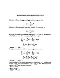
Figure 1: Comparison of mean, standard deviation and marginal probability for the enzyme-substrate model. In the three figures, we assume that 𝑛1 (0) = 5, 𝑛2 (0) = 5, and 𝐴 = 5. (a) shows the comparison of exact values and approximate values obtained from the PPGF method for mean and mean ± standard deviations (±𝜎) of 𝑛1 and (b) shows the comparison of the exact probability and the approximate probability obtained from the PPGF method. In the figure, 𝑃(𝑠 = 𝑖) denotes the probability that the number 𝑛2 of the substrate is 𝑖. The exact probability, mean, and variance are obtained by rewriting (15) into the linear ODE system 𝑑𝑝/𝑑𝑡 = 𝐾𝑝 under the given initial condition and then solving it by MATLAB.

simply make further elimination after the first truncation. By introducing the second truncation, we can alleviate the restriction on the original truncation in 𝑡 and allow higher order terms to remain, which is essential for computation of high order moments and probabilities. In the second truncation, the terms with relatively small coefficients are dropped. It is justified from the fact that the coefficient of each term in the PGF is the probability of a specific state. We can therefore carry over high order terms, while keeping a reasonable number of terms only. This is important since evaluation of the high order moments and the probabilities is generally expensive, especially when the system involves stiff chemical reactions. Since DTM can preserve the high order terms without increasing the total number of the terms, it enables us to easily evaluate the probabilities for the states with many molecules. The First Truncation. To overcome gradually increasing computational load in the series expansion (10), we restrict the series solution onto a short time interval. That is, on each interval [𝑡𝑟 , 𝑡𝑟+1 ], 𝑟 = 0, 1, 2, . . ., 𝑡0 = 0 < 𝑡1 < 𝑡2 < ⋅ ⋅ ⋅ , we construct the separate Taylor expansion 𝐺[𝑟] (z, 𝑡) at the center 𝑡 = 𝑡𝑟 of finite order 𝑁. We expect that side-by-side PGFs on consecutive intervals, 𝐺[𝑟] (z, 𝑡) and 𝐺[𝑟+1] (z, 𝑡), are equal on the boundary 𝑡 = 𝑡𝑟+1 as 𝐺[𝑟] (z, 𝑡𝑟+1 ) ≈ 𝐺[𝑟+1] (z, 𝑡𝑟+1 ) .

(20)

More generally, 𝑁

𝐺[0] (z, 𝑡) = ∑ 𝑓𝑛[0] (z) 𝑡𝑛 ,

𝐺[0] (z, 0) = zn ,

𝑛=0

𝑁

𝑛

𝐺[1] (z, 𝑡) = ∑ 𝑓𝑛[1] (z) (𝑡 − 𝑡1 ) , 𝑛=0

𝐺[1] (z, 𝑡1 ) = 𝐹 (𝐺[0] (z, 𝑡1 )) , 𝑁

𝑛

𝐺[2] (z, 𝑡) = ∑ 𝑓𝑛[2] (z) (𝑡 − 𝑡2 ) , 𝑛=0

𝐺[2] (z, 𝑡2 ) = 𝐹 (𝐺[1] (z, 𝑡2 )) ,

(21)

.. . 𝑁

𝑛

𝐺[𝑟] (z, 𝑡) = ∑ 𝑓𝑛[𝑟] (z) (𝑡 − 𝑡𝑟 ) , 𝑛=0

𝐺[𝑟] (z, 𝑡𝑟 ) = 𝐹 (𝐺[𝑟−1] (z, 𝑡𝑟 )) , .. . where 𝐹 is a “carry-over” functional. Our motivation of this successive superimpositions is to keep approximation order

Journal of Applied Mathematics

5 1

40 35 Probability

n2

25 20 15 10

0.6 0.4 P(y = 1) 0.2

5 0

P(y = 0)

0.8

30

0

100

200

300

400

0

500

P(y = 2) 0

5

10

15 Time

Time

20

25

30

SSA PPGF (b)

35 +𝜎

+𝜎

30 25 E[n2 ]

E[n1 ]

(a)

18 16 14 12 10 8 6 4 2 0

20 15 −𝜎

10

−𝜎

5 0

20

40

60

80 100 Time

120

140

160

0

0

20

40

60

80 100 Time

120

140

160

SSA PPGF

SSA PPGF (c)

(d)

Figure 2: Comparison of mean and standard deviation for the Brusselator model. The initial condition 𝑛1 (0) = 0 and 𝑛2 (0) = 0 are assumed. (a) shows a typical run of 𝑌 in 500 seconds from a Monte Carlo simulation of the Brusselator model. In (b), 𝑃(𝑦 = 𝑖) denotes the probability that the number 𝑛2 of the substrate is 𝑖. (c) and (d) compare mean and mean ± standard deviations (±𝜎) of 𝑛1 , 𝑛2 , and 𝑛3 obtained from the SSA and the PPGF. The results from the SSA are based on 50,000 realizations.

𝑁 low in favor of computational efficiency while carrying over essential information like first several moments to a next function over the following time interval. Note that truncation of high order temporal terms can be justified in that, in PGF computation, 𝑁 represents how many reaction would happen for that interval [𝑡𝑟 , 𝑡𝑟+1 ], 𝑟 = 0, 1, 2, . . .. Elimination of such terms has an effect of excluding excessive occurrence of reactions during such short interval. One of the issues in the first truncation is how to determine carry-over functional 𝐹. Although the best approximation in this framework would be obtained with the identity functional, it is not a practical choice since the number of terms involved in the computations keeps increasing rapidly. In [15], 𝐹 was suggested as a projection onto 𝑃3 (z), a set of polynomials of degree three or less, which preserves the mean and the variance. However, such functional does not preserve the information related to high order derivatives of PGF and therefore approximation of quantities such as the state probabilities is not possible. Here we propose a different type of carry-over functional that preserves high

order information. This functional indeed works as another truncation on what remains after the first truncation. The Second Truncation. At time 𝑡 = 𝑡𝑟+1 , the separate PGF 𝐺[𝑟] becomes ∞

𝐺[𝑟] (z, 𝑡𝑟+1 ) = ∑ zn 𝑝[𝑟] (n, 𝑡𝑟+1 ) ,

(22)

n=0

where 𝑝[𝑟] (n, 𝑡𝑟+1 ) means the probability for the state being n at time 𝑡𝑟+1 . Now we define the carry-over functional 𝐹 such that it maps (22) into ∞

∑ zn 𝐼𝜖 (𝑝[𝑟] (n, 𝑡𝑟+1 )) ,

(23)

n=0

where 𝐻𝜖 is a function defined as {𝑥, 𝐼𝜖 (𝑥) = { 0, {

if 𝑥 > 𝜖, if 𝑥 ≤ 𝜖.

(24)

Journal of Applied Mathematics 20 15 10 5 0

10 Variance

Mean

6

0

1

2

3

4

5

6

7

8

9

5 0

10

0

1

2

3

4

5

Time

6

7

8

9

10

Time

SSA DTM

SSA DTM

Probabilities

(a)

(b)

0.2 p(n2 = 5)p(n = 10) 2 0.15 0.1 0.05 0 0 1 2 3

p(n2 = 17)

4

5

6

7

8

9

10

Time SSA DTM (c)

Figure 3: The initial condition 𝑛 = [10, 20, 20, 0] and parameters 𝑐1 = 0.1, 𝑐−1 = 1, and 𝑐2 = 0.5 are assumed. In (c), each curve 𝑝(𝑛2 = 𝑖) denotes the time-dependent probability solution that 𝑛2 = 𝑖, 𝑖 = 5, 10, 17, respectively. The terms which have a coefficient less than 10−7 are dropped out.

Application of such 𝐹 implies that we sieve the terms out of which coefficients are less than 𝜖. One can see from (2) that those terms correspond to rare events of which coefficients probability is less than 𝜖. Considering that the iterative process in the PGF approach is a linear operation with respect to zn , manipulation on a term only affects entailed terms, each of which represents possible consequence of the corresponding state. Since the probabilities of all the entailed events and their sum as well cannot exceed the probability of the eliminated event, the effect of elimination does not propagate or grow in probability. Note that this truncation process is clearly consistent in that the scheme reverts to the first truncation as 𝜖 → 0. However, one should be careful when applying the second truncation to approximation of the moments, since the moments do not solely depend on the state probabilities. For example, suppose that a rare state eventually gives a birth to large number of a species in an open system. If the mean is what is sought, one cannot simply omit such state for the reason that the corresponding probability is small, since the elimination may substantially change the resulted mean or variance in approximation. Hence, for the moment approximation of the open systems, it is better to use the above functional 𝐹 together with other carry-over functional as suggested in [15]. 4.2. Example 1: Enzyme Kinetics. Once again, we use the enzyme kinetic model to test the performance of DTM. Figure 3 shows comparison of approximate solutions obtained from DTM and those from SSA. Note that, in the perturbation method in Section 3.2, evaluation of the probabilities was available only for the states that correspond to small number of that species, 𝑛2 = 0, 1, 2. This is

because the probability computation (8) requires as many times of differentiation as the number of the species at the state. However, one can see that DTM successfully resolves this problem and produces the probabilities of the states corresponding as many as 𝑛2 = 10, 15. 4.3. Example 2: 𝐺2 /𝑀 Transition Model. We consider the 𝐺2 /𝑀 transition network in the eukaryotic cell cycle as follows [14, 17]: 𝑐1

𝑐3

→ 𝑋𝑝 + 𝑌𝑝 , 𝑋 + 𝑌𝑝 󴀘󴀯 𝐶𝑥 󳨀 𝑐2

𝑐7

𝑐9

𝑋𝑝 + 𝑌 󴀘󴀯 𝐶𝑦 󳨀 → 𝑋𝑝 + 𝑌𝑝 , 𝑐8

𝑐4

𝑐6

𝐸1 + 𝑋𝑝 󴀘󴀯 𝐶𝑥𝑒 󳨀 → 𝑋 + 𝐸1 𝑐5

𝑐10

𝑐12

𝐸2 + 𝑌𝑝 󴀘󴀯 𝐶𝑦𝑒 󳨀󳨀→ 𝑌 + 𝐸2 . 𝑐11

(25) We denote the number of molecules of 𝑋𝑝 , 𝑌𝑝 , 𝑋, 𝑌, 𝐸1 , 𝐸2 , 𝐶𝑥 , 𝐶𝑥𝑒 , 𝐶𝑦 , and 𝐶𝑦𝑒 by 𝑛1 , 𝑛2 , 𝑛3 , 𝑛4 , 𝑛5 , 𝑛6 , 𝑛7 , 𝑛8 , 𝑛9 , and 𝑛10 , respectively. We obtain a PDE of the moment generating function 𝐺(z, 𝑡) [14] 𝐺𝑡 = 𝑐1 𝐺23 (𝑧7 − 𝑧2 𝑧3 ) + 𝑐2 𝐺7 (𝑧2 𝑧3 − 𝑧7 ) + 𝑐3 𝐺7 (𝑧1 𝑧2 − 𝑧7 ) + 𝑐4 𝐺15 (𝑧8 − 𝑧1 𝑧5 ) + 𝑐5 𝐺8 (𝑧1 𝑧5 − 𝑧8 ) + 𝑐6 𝐺8 (𝑧3 𝑧5 − 𝑧8 ) + 𝑐7 𝐺14 (𝑧9 − 𝑧1 𝑧4 ) + 𝑐8 𝐺9 (𝑧1 𝑧4 − 𝑧9 )

(26)

+ 𝑐9 𝐺9 (𝑧1 𝑧2 − 𝑧9 ) + 𝑐10 𝐺26 (𝑧10 − 𝑧2 𝑧6 ) + 𝑐11 𝐺10 (𝑧2 𝑧6 − 𝑧10 ) + 𝑐12 𝐺10 (𝑧4 𝑧6 − 𝑧10 ) . In Figure 4, we compare the simulation results obtained from the SSA and the DTM.

Journal of Applied Mathematics

7 1.5

3.8

Variance

Mean

4 3.6 3.4 3.2

0

0.2

0.4

0.6

0.8

1

1.2

1.4

1.6

1.8

1 0.5 0

2

0

0.2

0.4

0.6

0.8

Time

1 1.2 Time

1.4

1.6

1.8

2

Exact DTM

Exact DTM (a)

(b)

Probabilities

0.4 0.3

p(n2 = 5)

0.2

p(n2 = 3)

0.1 0

p(n2 = 1)

0

0.2

0.4

0.6

0.8

1

1.2

1.4

1.6

1.8

2

Time Exact DTM (c)

Figure 4: The initial condition 𝑛 = [5, 4, 2, 3, 2, 3, 2, 0, 0, 0] and parameters 𝑐1 = 𝑐4 = 𝑐7 = 𝑐10 = 0.2, 𝑐2 = 𝑐5 = 𝑐8 = 𝑐11 = 1, and 𝑐3 = 𝑐6 = 𝑐9 = 𝑐12 = 0.1 are assumed. In (c), each curve 𝑝(𝑛2 = 𝑖) denotes the time-dependent probability solution that 𝑛2 = 𝑖, 𝑖 = 1, 3, 5, respectively. The terms which have a coefficient less than 10−8 are dropped out.

5. Conlusion In this work, we presented the double truncation method (DTM) that improves the probability generating function (PGF) method for computation of the solutions of stochastic reaction networks. Advantage of the PGF method is that, rather than struggling with the chemical master equation of extremely high order, one can handle a partial differential equation (PDE) of low order. However, it still requires intense computation for high order approximation, especially for the systems with stiff parameters. The method proposed in this paper applies the perturbation method to the corresponding PGF for reaction networks. That is, we expand the PGF in the parameter that is responsible for stiffness of the system. Then the PGF-PDE leads to a recurrence relation of the coefficient functions with respect to both the time and the corresponding parameter, which we can easily solve symbolically. It turns out that the suggested method requires a lower approximation order than the original PGF method, while it produces as good approximation as such. While mean and variance of species are easily traceable in single truncation suggested in [15], efficient evaluation of the state probability was still a challenging task. In Section 4, we showed that the probability evaluation though PGF-PDEs can be achieved by doubly truncating the Taylor series at each time step. Through consecutive truncation processes, we dump relatively rare events, most of which are generated from excessive occurrence of reactions during a short time

interval. This also implies elimination of a great deal of terms and significant reduction in computation. It turns out in several numerical examples that the suggested method produces good approximation for the state probabilities. We expect that the DTM will be used for a fast and accurate approximation for computation of real and complex stochastic chemical reaction networks.

Conflict of Interests The authors declare that there is no conflict of interests regarding the publication of this paper.

Acknowledgments Pilwon Kim acknowledges that this work was supported by Basic Science Research Program through the National Research Foundation of Korea (NRF) funded by the Ministry of Education (2011-0023486). Chang Hyeong Lee was supported by Basic Science Research Program through the National Research Foundation of Korea (NRF) funded by the Ministry of Education (2014R1A1A2054976).

References [1] C. V. Rao, D. M. Wolf, and A. P. Arkin, “Control, exploitation and tolerance of intracellular noise,” Nature, vol. 420, no. 6912, pp. 231–237, 2002.

8 [2] D. T. Gillespie, “A rigorous derivation of the chemical master equation,” Physica A: Statistical Mechanics and its Applications, vol. 188, no. 1–3, pp. 404–425, 1992. [3] D. T. Gillespie, “Exact stochastic simulation of coupled chemical reactions,” Journal of Physical Chemistry, vol. 81, no. 25, pp. 2340–2361, 1977. [4] D. T. Gillespie, “Approximate accelerated stochastic simulation of chemically reacting systems,” Journal of Chemical Physics, vol. 115, no. 4, pp. 1716–1733, 2001. [5] Y. Cao, D. T. Gillespie, and L. R. Petzold, “Efficient step size selection for the tauleaping simulation method,” The Journal of Chemical Physics, vol. 124, no. 4, Article ID 044109, 2006. [6] D. F. Anderson, “Incorporating postleap checks in tau-leaping,” Journal of Chemical Physics, vol. 128, no. 5, Article ID 054103, 2008. [7] Y. Cao, D. T. Gillespie, and L. R. Petzold, “The slow-scale stochastic simulation algorithm,” Journal of Chemical Physics, vol. 122, no. 1, Article ID 014116, 2005. [8] B. Munsky and M. Khammash, “The finite state projection algorithm for the solution of the chemical master equation,” Journal of Chemical Physics, vol. 124, no. 4, Article ID 044104, 2006. [9] C. H. Lee and R. Lui, “A reduction method for multiple time scale stochastic reaction networks,” Journal of Mathematical Chemistry, vol. 46, no. 4, pp. 1292–1321, 2009. [10] C. H. Lee and R. Lui, “A reduction method for multiple time scale stochastic reaction networks with non-unique equilibrium probability,” Journal of Mathematical Chemistry, vol. 47, no. 2, pp. 750–770, 2010. [11] C. H. Lee, K.-H. Kim, and P. Kim, “A moment closure method for stochastic reaction networks,” Journal of Chemical Physics, vol. 130, no. 13, Article ID 134107, 2009. [12] P. Milner, C. S. Gillespie, and D. J. Wilkinson, “Moment closure approximations for stochastic kinetic models with rational rate laws,” Mathematical Biosciences, vol. 231, no. 2, pp. 99–104, 2011. [13] C. H. Lee, “A moment closure method for stochastic chemical reaction networks with general kinetics,” MATCH. Communications in Mathematical and in Computer Chemistry, vol. 70, no. 3, pp. 785–800, 2013. [14] P. Kim and C. H. Lee, “A probability generating function method for stochastic reaction networks,” Journal of Chemical Physics, vol. 136, no. 23, Article ID 234108, 2012. [15] P. Kim and C. H. Lee, “Fast probability generating function method for stochastic chemical reaction networks,” MATCH: Communications in Mathematical and in Computer Chemistry, vol. 71, no. 1, pp. 57–69, 2014. [16] D. A. McQuarrie, “Stochastic approach to chemical kinetics,” Journal of Applied Probability, vol. 4, pp. 413–478, 1967. [17] A. Kumar and K. Josi´c, “Reduced models of networks of coupled enzymatic reactions,” Journal of Theoretical Biology, vol. 278, pp. 87–106, 2011.

Journal of Applied Mathematics

Advances in

Operations Research Hindawi Publishing Corporation http://www.hindawi.com

Volume 2014

Advances in

Decision Sciences Hindawi Publishing Corporation http://www.hindawi.com

Volume 2014

Journal of

Applied Mathematics

Algebra

Hindawi Publishing Corporation http://www.hindawi.com

Hindawi Publishing Corporation http://www.hindawi.com

Volume 2014

Journal of

Probability and Statistics Volume 2014

The Scientific World Journal Hindawi Publishing Corporation http://www.hindawi.com

Hindawi Publishing Corporation http://www.hindawi.com

Volume 2014

International Journal of

Differential Equations Hindawi Publishing Corporation http://www.hindawi.com

Volume 2014

Volume 2014

Submit your manuscripts at http://www.hindawi.com International Journal of

Advances in

Combinatorics Hindawi Publishing Corporation http://www.hindawi.com

Mathematical Physics Hindawi Publishing Corporation http://www.hindawi.com

Volume 2014

Journal of

Complex Analysis Hindawi Publishing Corporation http://www.hindawi.com

Volume 2014

International Journal of Mathematics and Mathematical Sciences

Mathematical Problems in Engineering

Journal of

Mathematics Hindawi Publishing Corporation http://www.hindawi.com

Volume 2014

Hindawi Publishing Corporation http://www.hindawi.com

Volume 2014

Volume 2014

Hindawi Publishing Corporation http://www.hindawi.com

Volume 2014

Discrete Mathematics

Journal of

Volume 2014

Hindawi Publishing Corporation http://www.hindawi.com

Discrete Dynamics in Nature and Society

Journal of

Function Spaces Hindawi Publishing Corporation http://www.hindawi.com

Abstract and Applied Analysis

Volume 2014

Hindawi Publishing Corporation http://www.hindawi.com

Volume 2014

Hindawi Publishing Corporation http://www.hindawi.com

Volume 2014

International Journal of

Journal of

Stochastic Analysis

Optimization

Hindawi Publishing Corporation http://www.hindawi.com

Hindawi Publishing Corporation http://www.hindawi.com

Volume 2014

Volume 2014