subject to the following Kelly-MacLane coherence axioms [41, 39]: ...... QUEEN MARY AND WESTFIELD COLLEGE, UNIVERSITY OF LONDON, MILE END ...
Petri Nets and Other Models of Concurrency Mogens Nielsen and Vladimiro Sassone A BSTRACT. This paper retraces, collects, and summarises contributions of the authors — in collaboration with others — on the theme of Petri nets and their categorical relationships to other models of concurrency.
C ONTENTS Introduction Part 1. ON THE BEHAVIOUR OF NETS 1. Petri Nets, Hoare Structures, and Trace Structures 1.1. Elementary net systems 1.2. Trace structures 1.3. A categorical way to relationships 2. Petri Nets, Event Structures, and Domains 2.1. Event structures 2.2. Event structures and domains 2.3. Semiweighted nets 2.4. Unfolding semiweighted nets 3. Petri Nets and Transition Systems 3.1. Transition systems 3.2. Elementary nets and transition systems 4. Petri Nets and Bisimulations 4.1. Labelled models and their relationship 4.2. Path-lifting morphisms 4.3. PomL -bisimulation for nets Part 2. ON THE STRUCTURE OF NETS 5. Petri nets as monoids 5.1. Concatenable processes 5.2. Monoidal categories and concatenable processes 5.3. Axiomatising concatenable processes 6. Conclusions and Related Work Acknowledgements References 1991 Mathematics Subject Classification. Primary 68Q55, 68Q10, 68Q05. Key words and phrases. Semantics and Models of Concurrency, Noninterleaving, Petri Nets.
Introduction Concurrency theory is based on a number of different formal models of computation, with Petri nets [66, 67], or just nets, as a prominent example. Other models include the event structures of Winskel [94], the trace structures of Mazurkiewicz [43], the asynchronous and the concurrent transition systems of Bednarczyk [4], Shields [83] and Stark [84], just to name a few. Similarly, concurrency deals with an abundance of notions for behavioural equivalence, with the bisimulation of Milner [50], trace equivalence of Hoare [30], and pomset equivalence of Pratt [69] as prime examples. During the past decade, attempts have been made in order to understand the relationships between the confusingly many different concepts within concurrency theory, and many of these are based on the language of category theory. Our main goal in this paper is to survey some of the main ideas behind this categorical approach to concurrency, and at the same time to present some particular categorical results for nets. The first part of our paper is devoted to some categorical results on the behaviour of nets and their relations with other models, whereas the second part focuses on a categorical approach to the algebraic structure of net processes. In our presentation we have chosen to treat (only) three different classes of net systems: the elementary net systems of Thiagarajan [87], the semiweighted net systems [48], and place/transition systems [72], but the approaches presented here are, we claim, applicable to any class of net systems. Let us start by a few general comments on the role of category theory in our treatment of the behaviour of net systems. Fist of all, how do we relate nets to other models for concurrency? Any model for concurrency is meant to model the behaviour of distributed systems at a certain level of abstraction, focusing on certain aspects of the behaviour, deliberately abstracting from others. Here, we shall attempt to classify models according to their ‘level of abstraction’, and in stating and proving such relationships we shall use the language of category theory — in particular the notion of adjunction. In many contexts this has proven to be a convenient language succinctly expressing such relationships, abstracting away from the details of the often very different mathematical formalisms of the individual models. As the reader will see, nets relate nicely to most of our chosen models, in the sense that one of the models ‘embed’ into the other; ‘embedding’ is formalised here by special adjunctions called coreflections. As the reader will see, adjunctions and hence coreflections between two categories of models, M0 and M1 , consists of ways of translating from one model to the other, satisfying certain properties. Formally, an adjunction is expressed in terms of two functors L : M0 M1 and R : M1 M0 , and a coreflection is a way of saying that M0 embeds into M1 — with L telling us how to embed M0 into M1 , and R how to project M1 onto M0. This will be our formal way of saying that ‘M0 is an abstract version of M1’. In Part 1, we shall show examples of such embeddings between our classes of net systems and those of event structures, trace structures, domains, and transition systems. These result are part of a greater picture of relationships between models for concurrency, see e.g. [97, 80, 79]. We have chosen to present a few results in some detail, at the expense of the range of models covered. It is important to notice that all our categories are based on notions of morphisms which should be thought of as ‘simulations’. This view is supported by the fact that
!
!
they are all ‘behaviour respecting’, as formalised in concrete theorems. This means that the existence of a morphism may be seen as a demonstration that one object (implementation) satisfies another (specification), and hence morphisms may also play a role in formal verification. Once adjunctions are established between models, one may start comparing and transferring behavioural concepts from one model to another, formally via the adjoints L and R. In the final section of Part 1, we shall present on such example based on [35, 63], introducing a general way of understanding Milner’s seminal notion of bisimulation [50] across a range of different models, including net systems. It must be noted that there is more to the categorical view of models than we present here. For instance, universal constructs like products and coproducts serve as basis for giving semantics to process algebras. The reader is referred to [97] for more detail. In Part 2 we restrict attention to the level of single nets in order to analyse the structure of their spaces of computations, i.e., the algebraic structure of their processes. Of course, we keep using categorical tools, following an approach that can be said ‘in the small’, as opposed to the one in Part 1 that — dealing with the totality of nets — is ‘in the large’. The idea is, given a net N, to describe in abstract terms its concatenable processes, a notion introduced in [18] to account for sequential composition of processes. The existence of an operation of concatenation leads easily to a category of concatenable processes of N, where objects are states (markings) and arrows are (concatenable) processes. It turns out that such a category is a symmetric monoidal category whose tensor product is the parallel composition of processes [18]. The relevance of this result is that it describes Petri net behaviours as algebras in a remarkable way. Here we recall some of the results of [77, 18, 45, 75] providing, in particular, a construction that associates to each net N a symmetric monoidal category P (N ) isomorphic to the category of concatenable processes of N. Such an approach is completely abstract, axiomatic, in that it is formulated in terms of universal constructions. Namely, as we shall see, P (N ) is the free symmetric strict monoidal category on the net N modulo two simple additional axioms. The exposition is based on [77]. Most of the results presented here are based on work by the authors in co-operation with colleagues. Our main contribution here has been to collect and reformulate existing results, and to add a few new results as an attempt to obtain a uniform and coherent exposition. The results on elementary net systems and their relationships to other models in Part 1 is based on various works by G. Rozenberg, P.S. Thiagarajan, and G. Winskel in collaboration with Nielsen. The work on unfolding semiweighted nets and nets as monoidal categories are due to Sassone in collaboration with M. Meseguer, U. Montanari. And finally, Section 4 on nets and bisimulation is adopted from work A. Joyal, and G. Winskel and Nielsen. Part 1. ON THE BEHAVIOUR OF NETS 1. Petri Nets, Hoare Structures, and Trace Structures We start out be considering some fundamental and simple classes of Petri nets and their relationships to other models for concurrency. The theory of nets was originally a
strong source of inspiration behind the introduction of traces by Mazurkiewicz in [43]. Also, the relationship between traces and nets have been extensively studied, see in particular the survey papers by Rozenberg and Thiagarajan in [73, 87]. The presentation here is based on joint work with Rozenberg and Thiagarajan, [59], in which proofs and details may be found. 1.1. Elementary net systems. Elementary net systems were introduced by Thiagarajan [87] as a fundamental class of nets. His definitions were as follows. D EFINITION . A condition/event net (CE for short) is a triple (B E F ) where B and E are disjoint sets of, respectively, conditions and events, F (B E ) (E B), the flow relation, admits no isolated elements, i.e.,
� � � �
� � where domain F fx j 9y x y 2 F g and range F fy j 9x x y 2 F g. Let N B E F be a CE. Then X B � E is the set of elements of N. Let x 2 X . It will be convenient to use the following notation. x fy j y x 2 F g (the set of pre-elements of x) fy j x y 2 F g (the set of post-elements of x) x This ‘dot’ notation is extended to subsets of X in the obvious way. For e 2 E we domain(F ) range(F ) = B E
( )=
=(
:(
)
)
( )=
:(
)
N=
=
(
)
=
(
)
N
N
shall call e the set of pre-conditions of e and we shall call e the set of post-conditions of e. D EFINITION . A CE net is said to be simple if for all x y x = y , we have x = y.
2X
N
such that x = y and
D EFINITION . An elementary net system is a quadruple N = (B E F cin ) where . (B E F ) is a simple net called the underlying net of N. . cin B is the initial case of N.
�
Thus a simple CE net may be viewed as a directed bipartite graph with no isolated or confused elements, and an elementary net system is a simple net together with a ‘state’ specified as subset of B-elements. Presenting an elementary net system as a graph, following standard practise, the B-elements will be drawn as circles, the E-elements as boxes, the elements of the flow relation, F, as directed arcs, and the initial case will be indicated by dots (tokens) on its members. Figure 1 is an example of a net. As a model for concurrency, B-elements are used to denote the (local) atomic states (or resources) called conditions and the E-elements are used to denote (local) atomic changes-of-states called events. The flow relation models the effect on conditions by an occurrence of an event, in the form of a fixed neighbourhood relation between the conditions and events of a system. The dynamics of an elementary net system are simple. A state (usually called a case) of the system consists of a set of conditions holding concurrently. An event can occur at a case if all its pre-conditions and none of its post-conditions hold at the case. When an event occurs each of its pre-conditions ceases to hold and each of its postconditions begins to hold. Let us formalise this dynamics of net systems.
(/).*-+,F b1 xx FFF x FF x xx e1
GF
(/).*-+,
/
{
#
(/).*-+,
�
e3
e4
(/).*-+,DDb4
�
(/).*-+,
�
b3
�
DD zz DD zzz z e5 "
@A BC
b2
�
e2
b5
|
F IGURE 1
;! �
D EFINITION . Let N = (B E F ) be a net. Then P ow(B) N (elementary) transition relation generated by N, and is given by
;! f k e k j k r k 0
N = (
)
0
=
e
� E � P ow B
k0 r k = e
&
( )
is the
g
D EFINITION . Let N = (B E F cin ) be an elementary net system. .
.
CN , the state space of N, is the least subset of P ow(B) containing cin such that, 0 C . (Note that, whenever possible, we if c CN and (c e c0 ) N , then c N use N to denote both the net system and its underlying net.) CGN = (CN E CN ), is the case graph CN ), where CN = N (CN associated with N.
2
;!
2 ;! ;!
2 ;! \ � �
The case graph of N describes the dynamics of N by giving, for any possible state, the diagram of the possible state-transitions. Basic concepts concerning the behaviour of distributed systems such as causality, choice, concurrency, and confusion (‘glitch’) can now be cleanly defined — and separated from each other — with the help of net systems. The interested reader is referred to Thiagarajan [87] for details. Here we just bring out a few important behavioural concepts. E XAMPLE . Let us illustrate by means of a few small examples how nets can be used to model concurrency, nondeterminism, and enabling. (1) Concurrency: /) ( .* -+ ,
/) ( .* -+ ,
O
O
e1
e2 O
O
/) ( .* -+,
/) ( .* -+,
The events e1 and e2 can occur concurrently, in the sense that they both have concession and are independent in not having any pre or post conditions in common. (2) Conflict:
/) ( .* -+ ,
/) ( .* -+ ,
O
O
e1
e2
FF FF xx FF xxx x c
/) ( .* -+,
Either one of events e1 and e2 can occur, but not both. This shows how nondeterminism can be represented in a net. (3) Contact: /) ( .* -+ ,
/ /
/) ( .* -+,
/) ( .* -+ , / /
e1
e2
The event e2 has concession. The event e1 does not — its post condition holds — and it can only occur after e 2 . This illustrates contact. In general, there is contact at a marking M when for some event e e
�M
&
e
\ Mr e 6 (
)=
?
:
As a further example, a critical region may be described as the elementary net system in Figure 2, where the condition in the center represents a kind of semaphore controlling the access (p’s and v’s events) to critical regions (c 0 and c1 ) by the two processes.
(/).*-+,
GF
(/).*-+,
/
ED
o
w0
w1
(/).*-+, p0
(/).*-+, `
p1 >
(/).*-+,
(/).*-+, (/).*-+,
c0
N
c1
P
(/).*-+,
(/).*-+,
@A v0 BC
@A F IGURE 2
v1
BC
1.2. Trace structures. An traditional way to describe the behaviour of a system is to consider all the admissible sequences of event occurrences, the so-called traces of the system. Essentially, this amounts to giving a formal language whose alphabet is a set of events and whose strings represent the potential evolution of the system. Trace structures, introduced originally by Mazurkiewicz [43] as a model for concurrency, arose from a simple, yet powerful new idea: equip the alphabet of formal languages with an extra structure of independence, interpreted as computational independence between atomic actions. We recall this development starting with the following simpler notion. D EFINITION . A Hoare structure is a pair (H Σ) where Σ is an alphabet (of atomic actions), and H is a nonempty, prefix closed subset of the monoid Σ � . Actually, such structures are called traces in [30], but we prefer to reserve the word traces for the structures that will follow. Building on the definition of the transition relation we may associate an obvious Hoare structure with an elementary net system. D EFINITION . The set FSN of firing sequences of N = (B E F cin ) is the subset of E � defined inductively as follows. . ε FSN and cin ��ε cin , for ε the empty sequence;
2 ρ 2 FS
i
i
and cin ��ρ c and c
N
;! e
N
c0
2 FS and c ρei c Observe that i is the natural ‘extension’ of ;! to fc g� E � C . .
ρe
0
in ��
N
.
��
N
�
in
N
For the elementary net representation of the familiar example of mutual exclusion, we get the following Hoare structure
fε w
0
w1 w0 w1 w1 w0 w0 p0 w1 p1 w0 w1 p0
:::
g
:
One of the essential aspects of nets is that they allow an explicit representation of the distributed nature of computations. For instance, in the mutual exclusion example of Figure 2, the independence between actions w 0 and w1 is represented, following our intuitive understanding of the net, by the disjointness of their local effects. However, as with Hoare structures in general, firing sequences ‘hide’ aspects of the behaviour of a net system to do with parallel or independent activities. To bring out this deficiency more clearly, we follow the original way of introducing independence between events of elementary net systems. In net theory this relation is most often referred to as the concurrency relation.
6
2
2
D EFINITION . For e1 = e2 E and c CN , say that e1 and e2 can occur concurrently at c — written c�� e1 e2 or, when c can be omitted, also e1 co e2 — if c��e1 , c��e2 , and ( e1 e1 ) ( e2 e2 ) = ?.
f
� \ �
gi
i
i
Thus e1 and e2 can occur concurrently at c iff they can occur individually and their neighbourhoods are disjoint. Conflict is clearly the ‘dual’ notion: e 1 and e2 are in conflict at c if c��e1 , c��e2 , but not c�� e1 e2 , i.e., at c either e1 may occur or e2 may occur but not both. The choice as to whether e 1 or e2 will occur is assumed to be resolved by the ‘environment’ of the system. For the system N of Figure 1, for instance, at the initial case e1 and e4 can occur concurrently. Consequently, the
i
i
f
gi
|| ||
ε] B BB B
w1 ] BB BB BB BB || | | w0 p0 ] w0 w1 ] w1 p1 ] BB BB BB BB BB BB || || || | | | | | | w0 p0 c0 ] w0 w1 p0 ] w0 w1 p0 ] w1 p1 c1 ]
|| ||
w0 ]
F IGURE 3 firing sequences e1 e2 e4 and e4 e1 e2 and e1 e4 e2 all represent the same (non-sequential) stretch of behaviour of N. Also, e1 and e3 are in conflict at the initial case. Hence the firing sequences e1 e2 e4 and e3 e4 e5 represent two conflicting (alternative) stretches of behaviour of N. The idea suggested by Mazurkiewicz [43] is to allow the modelling of such independent activities of components of system by introducing the extra structure of an independence relation I on the action alphabet. For nets, following our intuition we would relate two actions as independent if and only if they involve concurrent events. Based on an independence alphabet, the behaviour of a system will be modeled in terms of traces, i.e., of equivalence classes of
hI
: the least congruence on E � such that e0 e1 hI e1 e0
'
f
whenever e0 I e1 :
g
In our running example w 0 w1 p0 I w0 p0 w1 and the equivalence class of w0 w1 p0 is �w0 w1 p0 ] = w0 w1 p0 w0 p0 w1 w1 w0 p0 . Now, Hoare structures generalise from subsets of Σ� to subsets of the monoid of traces, denoted M (Σ I ). The prefix ordering of Hoare structures generalise to a prefix ordering of traces, defined in terms of the following preorder on strings: s .I t
if and only if
9u su h t :
I
which induces the following partial order (prefix order) on traces:
v
I =
that is, �s ]
v
v
I �t ]
v
.I hI
if and only if
v
=
9u v s h u . v h t :
I
I
I
:
In our example �ε] I �w0 ] I �w0 w1 ] I �w0 p0 w1 ], and the initial traces and their prefix ordering are as shown in Figure 3. Notice that the extra modelling power boils down to the presence of traces like �w0 w1 ] in our example, representing actions w0 and w1 in any (unspecified) order, and interpreted as their concurrent or independent occurrences. We are now ready for our formal definition of trace structures. Conceptually, we follow [44] where a trace structure is defined to be a prefix closed, proper subset of the monoid M (Σ I ). However, only for technical reasons we prefer in our formal definition to work with such structures in terms of consistent subsets of Σ� — with the traces a derived notion, as in Proposition 1.1 below.
D EFINITION . A trace structure is a triple T = (M Σ I ) where (Σ I ) is an independence alphabet, i.e. I Σ Σ is irreflexive and symmetric, and M Σ� is such that for all t t 0 Σ� and a b Σ:
� � 2
2
�
) t 2 M; ) t 2 M; ) tab 2 M
2 2
consistency: t hI t 0 M prefix closure: ta M properness: ta tb M & a I b
2
=
= =
We use the notation M =hI for the traces of T , i.e., M =hI
f j w 2 Mg
= �w]
:
:
We may think of a trace structure as a prefix closed set of traces, in the sense that from the axioms of consistency and prefix closure above, we get the following. P ROPOSITION 1.1. Given a trace structure T . w M if and only if �w] M =hI ; .
2 w v
� ]
0 I �w ]
2
2M h =
implies
I
�w]
= (M
Σ I ) then (M =hI
v
I)
satisfies
2M h . =
I
As will be expected by now, the information concerning concurrency and conflictresolution hidden by Hoare structures may be retrieved by associating with a net a trace structure with concurrency as the appropriate independence relation. T HEOREM 1.2. Let N = (B E F cin ) be an elementary net system and let the independence relation associated with N be I=
fe
( 1
j
e2 ) e1 e2
2 E & e �e \ e �e ( 1
1)
( 2
2) =
?g
:
Then nt(N ) = (FSN E I ) is a trace structure. P ROOF. The required properties follow from definition. In particular, nt(N ) is consistent and proper by definition of the (elementary) transition relation. For the net system N from Figure 1, Figure 4 shows an initial portion of the associated poset of traces.
fe1 e2 e3OgO fe1 e2 e4 oe1 e4 e2OOe4 e1 e2 g fe3 e4 e5 e4 e3 e5 g OOO OOO oo o OO O o O oo fe1 e2 gOO fe1oe4 e4OeO1 g fe3oe4 e4 e3 g OOO OOO oo oo o o OO O o o O oo oo fe1 gOO fe4 g gfe3 g OOO oo ggggggggg o o OO oooggggg g fεgg F IGURE 4 The beauty of the trace semantics is its simplicity. One of the classical results from concurrency theory is that the trace semantics is ‘consistent’ with an alternative way of defining the behaviour of net systems in terms of unfoldings into processes (or occurrence nets). Several results of this type have been shown [9]. The presentation
that follows is adapted from [59]. For the sake of convenience we shall assume here that N is contact-free. In other words, we shall assume,
8c 2 C 8e 2 E e � c ) e \ c r e N:
(
=
:
)=
?
:
As we shall see later, this does not involve any loss of generality, at least for the study of behavioural issues. The theoretic development of Petri nets, focusing on the noninterleaving aspects of concurrency, brought to the foreground various notions of process, e.g. [68, 26, 7, 45, 18]. Generally speaking, these are structures accounting for the causal relationships which rule the occurrence of events in computations. Thus, ideally, processes are simply computations in which explicit information about such causal connections is added. Abstractly, the processes of a net N are ordered sets whose elements are labelled by events of N. Concretely, in order to describe exactly which sets of events give rise to processes, one takes a process of N = (B E F cin ) will be a labelled net of the form N˜ = (B˜ E˜ F˜ π), where (B˜ E˜ F˜ ) is a restricted kind of a net (viz., finite, conflict-free, acyclic) called a causal or process net, and the labelling function π : B˜ E˜ B E is required to connect the structure of N˜ to that of N in a suitable way. For a definition of a process along these lines see Part 2, or, e.g., [73]. Here we shall define processes with the help of firing sequences. This will enable us to build up the finite processes of N inductively. For a similar development of the process notion, see [9].
� ! �
For each firing sequence ρ, we will define a process Nρ = (Bρ Eρ Fρ πρ ). In doing so it will be convenient to keep track of the conditions that hold in N after the run represented by the firing sequence ρ. This set of conditions will be encoded as c ρ . D EFINITION . Let N be (B E F cin ). Then Nρ = (Bρ Eρ Fρ πρ ) is defined inductively on the length of ρ FSN as follows. Case ρ = ε: Then Nε = (? ? ? ?) and cε = (b φ) b cin .
2
f
j 2 g
Case ρ = ρ0 e: Assume that Nρ = (Bρ Eρ Fρ πρ ). Then Nρ = (Bρ Eρ Fρ πρ ) where, for X = (b D) b e & (b D) cρ and Y = (b (e X ) ) b e , we have
f
j 2 2 g f f E �f e X g B � X �Y F � X �f e X g � f e X g� Y λ z Z 2 B �E z r X � Y. 0
=
ρ0
=
ρ0
=
ρ0
πρ
=
(
0
0
0
0
0
Eρ Bρ Fρ
Finally, cρ = (cρ
0
(
)
(
)
gj 2 g
(
ρ
) )
ρ:
( (
)
)
:
)
It will turn out that Nρ as defined above is a labelled net. For ρ = e1 e2 e4 e3 in the system N of Figure 1 we show Nρ in Figure 5. For convenience we have displayed π ρ by writing the value of πρ (x) besides the graphical representation of x for each x B ρ Eρ . In order to establish a relationship between the traces of N and its processes it is necessary to define an ordering relation over the processes of N.
2 �
D EFINITION . Let N be (B E F cin ).
b1
/) ( .* -+ ,
/) ( .* -+ ,
e1
b2 e4
b3
/) ( .* -+ ,
/) ( .* -+ ,
b5
e2 b1
NNN NNN NNN e3
/) ( .* -+ ,
&
b4
/) ( .* -+ ,
F IGURE 5 .
.
f j 2 FS g, for N
The set of finite processes of N is PN = Nρ ρ definition. PN PN is defined by
v� �
(Bρ
Eρ Fρ πρ )
v
v
(Bρ0
Eρ Fρ πρ ) if Bρ 0
0
0
�B
ρ
N
ρ0
& Eρ
�E
ρ0
as in the previous
& Fρ
�F
ρ0 :
Clearly is a partial ordering relation. The main result relating trace semantics to processes is the following.
v
T HEOREM 1.3. For N any elementary net system (PN ) and the ordering of the traces from nt(N ), i.e., (FSN =hI I ), are isomorphic posets.
v
P ROOF. In [59] it is proved that f : FSN =hI morphism.
! P given by f
(�ρ]) =
Nρ is an iso-
1.3. A categorical way to relationships. In the last section we attempted to show connections between net systems and other structures. Although it is apparent that nets a more general, expressive, and powerful model, we lack at this stage a way to make precise any statement in this sense. Is there a formal way of saying that traces ‘embeds’ into nets, that ‘nets generalise’ them naturally? More generally, how can we relate nets to the other models? How do we establish relationships between models? As we discussed in the introduction, we tend to classify models can for concurrency according to their ‘level of abstraction’ (see, e.g., [80, 97, 79]), that is, according to those aspects of the behaviour of distributed systems they focus on and those they deliberately abstract from. In stating and proving relationships between models viewed under this perspective, the language of category theory as proven in many contexts to be very useful, as it is capable of abstracting away from unwanted details of the individual models and, therefore, of expressing the more essential aspects succinctly and in great generality. Let us review very briefly a few key steps behind these ideas.
First, all the models are introduced as a class of objects, e.g., the class of net systems or the class of trace structures, equipped with a notion of ‘behaviour-preserving’ (i.e., simulation) morphism, making each model into a category. The role of the morphisms is to make explicit (if and) how each single object relates to all the others. In particular, as behaviour is preserved, (if and) how it can be simulated. This makes explicit that central to our objects and, therefore, to the respective categories, is the dynamic notion of behaviour. Also, the very notion adopted for ‘simulation’ determines what aspects of behaviour are important, i.e., what can be ignored by a successful simulation (the aspects abstracted away) and what instead must be preserved (the aspects focused on). In other terms, the adopted notion of morphism define the abstraction level of the model. From this standpoint, the notion of functor is the first tool category theory makes available to us in order to check the sanity of our translations from one model to another. Essentially, it requires us to map objects to objects preserving all the existing relationships, i.e., all the existing simulations. In other words, it requires to map also behaviours to behaviours. Tools much more refined than functors are the notions of adjunction and coreflection, central to many papers on models of concurrency and, in particular, to our presentation here. Let us briefly comment on their formal definition and the intuitive way to understand them. Technically, an adjunction between categories M 0 and M1 , consists of ways of mapping from one to the other and back, satisfying certain properties. Formally, (see [42] for alternative characterisations) we shall express an adjunction in terms of two functors L : M0 M1 (the left adjoint) and R : M1 M0 (the right adjoint of the adjunction) satisfying (see Figure 6):
!
u
m0 f0
!
L (m0 )
RL(m0 ) R ( f1 )
R
R(m1 )
! f1 m1
M1
M0 F IGURE 6
!
for each object m0 of M0 , there is a morphism u : m0 R L(m0) (the unit at m0 ) such that for each object m1 of M1 and each morphism f0 : m0 R(m1 ), then there is a unique morphism f 1 : L(m0 ) m1 , such that f0 = R( f1 ) u. In other terms, for each m0 M0 , L(m0 ) is a ‘special’ object of M1 in the sense that all the maps from m to objects of the kind R(m 1 ) in M0 come exactly and unambiguously from maps from L(m0 ) to m1 in M1 . Moreover, all such maps can be factored in the image of R via u : m0 R L(m0 ), a ‘special’ map that m0 comes equipped with. Reading system for object and simulation for morphism, this definition has an evident significance in computational terms.
!
2
!
!
If all units of an adjunction are isomorphisms, then the adjunction is called a coreflection. This essentially means that no information is lost moving from M 0 to M1 , as the identity of objects is retained and recovered back by R. It follows from the definition that the left adjoint L of a coreflection is always full and faithful, i.e., an embedding. In other words, we may think of M 0 as a coreflective full subcategory of M1 (the one identified by the image of L), and of L as the inclusion M 0 , M1 , whereas R tells us how to project M1 back onto M0 . Paraphrasing this situation in terms of categories of models, behaviours and simulations, we can say that R selects for each m M1 its best possible abstract ‘approximation’ in M0 . That is, an object R(m) M0 together with a simulation R(m) m such that any other R(m0 ) m factors as R(m0 ) R(m) m. So much for the formal definition. In the following the existence of a coreflection of M0 into M1 will be our formal way of saying that ‘M 0 is an abstract version of M1 ’.
!
2
!
2
!
!
!
We therefore start by turning our models into a categories by defining appropriate notions of morphisms. Morphisms of languages are simply functions on their alphabets which send strings in one language to strings in another. D EFINITION . A function λ : Σ
! Σ extends to strings by defining 0
bλ(sα) = bλ(s)λ(α)
!
:
!
A morphism of Hoare structures (H Σ) consists of a function λ : Σ Σ0 0 b such that s H : λ(s) H . We write H for the category of Hoare structures with the above understanding of morphisms, where composition is our usual composition of functions.
82
2
(H 0
Σ0 )
Before we continue, let us comment briefly on our choice of morphisms — on Hoare structures as well as on all other models considered in this paper. In much of the literature, more liberal notions of morphisms are used, based on partial (rather than total) functions on the labelling sets. These more general morphisms have the advantage that many useful combinators (e.g., parallel composition) may be expressed as universal constructions in the corresponding categories of models. Furthermore, they may be thought of as specifying correctness properties: the ‘correctness’ of the mutual exclusion example, for instance, follows by the fact that the partial function λ from the alphabet of actions, which is undefined for w 0 w1 and the identity function for all other action symbols, is a morphism from the Hoare structure of the mutual exclusion example to the Hoare structure consisting of all prefixes of the regular language ( p0 c0 v0 + p1 c1 v1 )� . However, we have chosen here to restrict ourselves to morphisms based on total functions, purely as an attempt to simplify our presentation technically.
f
g
Similarly, morphisms between trace structures are morphisms between the underlying languages which preserve independence.
!
D EFINITION . A morphism of trace structures (M Σ I ) (M0 Σ0 I 0 ) consists of a 0 function λ : Σ Σ which preserves independence: α I β implies λ(α) I0 λ(β), for all α β Σ; preserves strings: s M implies bλ(s) M0 , for all strings s. This, with the usual composition of functions defines T, the category of trace structures.
!
2
2
2
It is easy to see that morphisms of trace structures preserve traces and the ordering between them.
!
(M 0 Σ0 I 0 ) be a morphism of trace structures. P ROPOSITION 1.4. Let λ : (M Σ I ) If s .I t in the trace structure (M Σ I ) then bλ(s) .I bλ(t ) in (M 0 Σ0 I 0 ). 0
It follows that bλ defines a monote function from (M =h I cerning nets, we consider the following definition.
v
I ) to (M
0=
hI
0
v
I 0 ).
Con-
D EFINITION . Let N = (B E F cin ) and N 0 = (B0 E 0 F 0 c0in ) be elementary net systems. A morphism (β η) : N N 0 consists of a relation β B B0 , such that βop is a partial function B0 * B, and a function η : E * E 0 such that
! � � 8 b b 2 β b 2 c () b 2 c β e ηe βe ηe Thus morphisms on nets preserve initial cases and events when defined. A morphism β η : N ! N expresses how occurrences of events and conditions in N induce (
(
0
)
)
occurrences in
:
in
0
0 in
( )=
( )
(
)=
( )
:
0
N0.
Morphisms on nets preserve behaviour.
P ROPOSITION 1.5. Let N = (B E F cin ) and N 0 = (B0 E 0 F 0 c0in ) be elementary nets N 0 a morphism. and (β η) : N 0 0 0 . If c ��e c in N, then f β (c) ��η(e) f β (c ) in N , for f β (c) = β(c) (c0in r β(cin )). .
! i If e \ e 1
2=
? in N, then
i
η(e1 )
\ηe
( 2) =
�
? in N 0 .
P ROOF. It is easily seen that η(e) = β( e) and that η(e) = β(e ) for all events e of N. Observe too that because βop is a partial function, β in addition preserves intersections and set differences. These observations mean that β(c) ��η(e) β(c 0 ) in N 0 follows from the assumption that c ��e c0 in N, and that independence is preserved.
i
i
D EFINITION . Let EN denote the category of elementary net systems and their morphisms under the obvious componentwise composition of morphisms, e.g., the composition of (β0 η0 ) : N0 N1 and (β1 η1 ) : N1 N2 is (β1 β0 η1 η0 ) : N0 N2
!
!
!
This choice of morphisms for elementary net systems may not be as obvious and intuitively clear as the those for the other models we consider. Indeed alternative categories of net systems have been studied — see, e.g., [93, 45, 12, 48, 97]. Here we just remark that Proposition 1.5 proves that these morphisms preserve behaviour (and concurrency), a fact that has been explored by, e.g. [11], where such morphism have been used to express correctness properties. Also, we note that the derived notion of isomorphism becomes identity up to names of conditions and events. T HEOREM 1.6. The construction that maps N E ) extends to a functor nh from EN to H.
= (B
E F cin ) to the Hoare structure
(FSN
T HEOREM 1.7. The trace semantics nt extends to a functor nt from EN to T. However, these functors are not part of any adjunction. Following our discussion above, one would expect a formal result embedding T in EN, but for this to be the case it turns out that one needs a more abstract semantics. The reason why nt is too concrete is that it preserves information about event ‘identities’. As we shall see in the next section, forgetting these will help yielding a ‘nice’ (read ‘universal’) unfolding of EN into event structures.
2. Petri Nets, Event Structures, and Domains Consider again the prefix ordering of traces introduced above. What can be said about their structure and properties? In this section we shall provide a characterisation of such orderings in terms of a well-known class of Scott domains [81, 6]. Moreover, in the process of doing so, we shall also show that they arise exactly as the orderings associated with the dynamics of another well-known model for concurrency: the event structures, originally introduced in [57]. 2.1. Event structures. The prefix ordering of the strings of a Hoare structure — which is in fact a tree ordering — may also be viewed as a structure over action occurrences, where individual occurrences may be either ordered, i.e., following each other in time in the same computation, or not, i.e., belong to different computations. Event structures may be seen as a generalisation of such structures, allowing a third relationship between occurrences, that of concurrency, i.e., belonging to the same computation, but without any causal/temporal ordering.
�
#) consisting of a set D EFINITION . Define an event structure to be a structure (E E, of events which are partially ordered by , the causal dependency relation, and a binary, symmetric, irreflexive relation # E E, the conflict relation, which satisfy for all e e0 e00 E
� � �
2
fe j e � eg is finite e # e � e ) e # e Say two events e e 2 E are concurrent, and write e co e , if : e � e or e � e or e # e Write __ for # � 1 , i.e., the reflexive closure of the conflict relation. 0
0
0
00
0
00
=
0
(
:
0
0
0 ).
E
The finiteness assumption restricts attention to discrete processes where an event occurrence depends only on finitely many previous occurrences. The axiom on the conflict relation expresses that if two events causally depend on events in conflict then they too are in conflict. Guided by our interpretation we can formulate a notion of computation state of an event structure (E #). Taking a computation state of a process to be represented by the set x of events which have occurred in the computation, we expect that
�
e0
2x
&
e
�e
)
0
=
e
2x
i.e., if an event has occurred then all events on which it causally depends have occurred too, and also that
8e e 2 x : e # e 0
:
(
0
)
i.e., two conflicting events cannot occur together in the same computation.
� � # , are 8 2 : downwards-closed: 8e e e � e 2 x ) e 2 x. In particular, define bec fe 2 E j e � eg, which is a configuration, as it is downwardclosed and conflict-free. Write D E � # for the set of finite configurations. D EFINITION . Let (E #) be an event structure. Its configurations, D (E those subsets x E which are conflict-free: e e0 x: (e # e0 );
�
0: 0
=
0
=
0
0(
)
0
)
The important relations associated with an event structure can be recovered from its finite configurations (or indeed similarly from its configurations).
�
#) be an event structure. Then P ROPOSITION 2.1. Let (E 0 . e e if and only if x D 0 (E #): e0 x = e
�
.
e # e0
.
e co e0
8 2 � 2 ) 2 x; if and only if 8x 2 D E � # e 2 x ) e 2 x; if and only if 9x x 2 D E � # such that e 2 xrx & e 2 x rx & x�x 2 D E � # 0(
0
0
):
0(
0
=
0
=
)
0
0
0
(
):
Events manifest themselves as atomic jumps from one configuration to another, and later it will follow that we can regard such jumps as transitions in the case graph associated with a net system.
�# x ;! x
D EFINITION . Let (E
)
0
e
be an event structure and x x0 be configurations. Write if and only if e
2x & x =
0
=x
�feg
:
P ROPOSITION 2.2. Two events e0 e1 of an event structure are in the concurrency relation co if and only if there exist configurations x x0 x1 x0 such that x0 ? e e1 ?? 0 ? x0 ? x1 ?? e0 ? e1 x ?
_
?
_
Morphisms on event structures are defined as follows [92, 91]:
� )
#) and ES0 = (E 0 D EFINITION . Let ES = (E 0 phism from ES to ES consists of a function η : E x
2 D ES (
)
=
!
2 D ES 8e e 2 x η e η(x)
0)
(
0
1
:
� # be event structures. A mor! E on events which satisfies 0
0
0)
)e
( 0 ) = η(e1 ) =
0 = e1 :
A morphism η : ES ES0 between event structures expresses how behaviour in ES determines behaviour in ES 0 . The function η expresses how the occurrence of events in ES implies the simultaneous occurrence of events in ES 0 ; the fact that η(e) = e0 can be understood as expressing that the event e 0 is a ‘component’ of the event e and, in this sense, that the occurrence of e implies the simultaneous occurrence of e 0 . If two distinct events in ES have the same image in ES 0 under η then they cannot belong to the same configuration. Morphisms of event structures preserve the concurrency relation. This is a simple consequence of Proposition 2.2, showing how the concurrency relation holding between events appears as a ‘little square’ of configurations. P ROPOSITION 2.3. Let E be an event structure with concurrency relation co and E 0 an event structure with concurrency relation co0 . Let η : E E 0 be a morphism of event structures. Then, for any events e0 e1 of E,
!
e0 co e1
)
=
η(e0 ) co0 η(e1 ):
Morphisms between event structures can be described more directly in terms of the causality and conflict relations of the event structure. P ROPOSITION 2.4. A morphism of event structures from (E function η : E E 0 such that . η(e) η( e ), .
! b c� b c η e __ η e ) ( 0)
0
( 1)
=
e0
�#
)
to (E 0
�
0
#0 ) is a
__ e . 1
Let E denote the category of event structures with morphism as described above and composition named composition of functions. 2.2. Event structures and domains. Let us turn our attention to the class of partial orders corresponding with the orderings of configurations of event structures. The characterisation given below in terms of special Scott domains has been originally formulated in [57]. In the following, we shall need a few standard definitions from theory. For F X domain (D ) a partial order and X a subset of D, we write as usual for the least upper bound of X, when it exists.
v
D EFINITION . Let (D such that
v be a partial order. A complete prime of D is an element p 2 D G p v X ) 9x 2 X p v x )
F for any set X for which X exists.
=
:
v
2
D EFINITION . For (D ) a partial and d0 d1 D, we say that d1 covers d0 , in symbols d0 < d1 , if and only if d0 @ d1 and, for every d,
v
d0
vdvd ) d 1 =
= d0
or d = d1 :
D EFINITION . Let (D ) be a partial order. We say that D is . bounded complete if all subsets X D which have an upper bound in D have a F least upper bound X in D. . coherent if all subsets X D which are pairwise bounded (i.e., such that all pairs of elements d d X have upper bounds in D), have least upper bounds 0 1 F X in D. (Note that coherence implies bounded completeness). . prime algebraic if
2
x=
for all x
G
�
�
f p v x j p is a complete primeg
2 D. If furthermore the sets f p v q j pis a complete primeg
are always finite when q is a complete prime, then D is said to be finitary. A prime algebraic domain domain is a bounded complete and prime algebraic partial order.
�
� �
T HEOREM 2.5. Let (E #) be an event structure. The partial order (D (E #) ), that we shall indicate simply as D (E #), is a coherent, finitary, prime algebraic domain whose complete primes are the e e E .
� fb c j 2 g
P ROOF. See [57, 95]. Conversely, any coherent, finitary, prime algebraic domain is associated with the partial order of configurations of event structures.
v
T HEOREM 2.6. Let (D ) be a coherent, finitary, prime algebraic domain. Define ) as the event structure (E #)
P r (D
v
Then (D
v
)
E
�
=
#
=
=
and D (E
�
v
the complete primes of (D ) is the restriction of to E (x y) E E x y does not exist in D
v 2 � j t
f
�#
)
g
are isomorphic partial orders.
P ROOF. See [57]. Actually, the relationship between event structures and coherent, finitary prime algebraic domains is very strong, in that they are equivalent: one can be used to represent the other. This may be formalised also in terms of a categorical equivalence between D and a category of coherent, finitary prime algebraic domains equipped with stable functions as morphisms. T HEOREM 2.7. Let D denote the category of coherent, finitary prime algebraic domains with morphism functions f : (D0 0 ) (D1 1 ) satisfying:
v ! v additivity: for all x y 2 D such that x t y exists, f x t y stability: for all x y 2 D such that x t y exists, f x u y covering preserving: for all x y 2 D if x y then f x
tf y ; f x uf y ;
0
(
)=
f (x)
( )
0
(
)=
( )
( )
0:
0, .
.
�
�
2 J� � S Co B ∑ b pre B t 2 T and pre B t ∑B t B t 2T post t ∑ b ; � ft g b 2 S 8 j 2 J and post t ∑ ;ft g b � B=
(x j
b j) � j 0=(
j
( )
k;1
(
0
.
2
� � � S0 = (? b) � b 2 uN ; T0 = ?, and pre0 and post0 with the obvious definitions;
)
)
j 2J
k(
k
N( ) =
k
uk = ∑ j (? b j ) = ∑ S0 = u0 .
N (t )
for t
2T
N
)=
j 2J
k ( 0) =
k
j=
j j
0
j
Therefore U (N )(0) consists of the initial marking of N, and, informally speaking, U (N )(n+1) is obtained, inductively, by generating a new transition for each possible subset of concurrent places of U (N )(n) whose corresponding multiset of places of N is the source of some transition t of N; the target of t is then decorated with its history and added to U (N )(n+1) . Clearly, we shall take U (N ) to be the colimit of the sequence of the U (N )(n) , n ω. To do that, we first need to prove the following lemma.
2
2
L EMMA 2.12. For all n ω U (N )(n) is an occurrence net of depth n. Moreover, for each n ω there is an inclusion inn : U (N )(n) U (N )(n+1) .
2
!
P ROOF. That U (N )(n) has depth n and that there exists an inclusion from U (N )(n) to U (N )(n+1) is obvious from the definition. We have to show that U (N )(n) is an occurrence net. For each t Tn , pren (t ) and postn (t ) are multisets where all the elements have multiplicity one, i.e., sets. The same happens for u n .
2
2
i) For each (x b) Sn , (x b) = x which is either the empty set or a singleton. So (x b) 1. Moreover, (x b) u n if and only if x = ? if and only if (x b) = ?. ii) By definition of U (N )(n) , whenever x 1 y 1 z, depth(z) = depth(x) + 1. Since x z Tn or x z Sn implies that there exists at least one y such that x y 1 z we have depth(x) < depth(z). So x = z and is irreflexive. Observe that this, together with (i), implies that, in each reachable marking, every place has multiplicity at most one. In fact, since that happens in u n , since each place has only one pre-event and each transition occurs at most once in any computation, there is no way to generate multiple tokens in a place. Moreover, t 0 Tn t 0 t is obviously finite for all t Tn . iii) Recall that x # x if and only if t t 0 Tn t = t 0 and t #m t 0 such that t x and t 0 x. So, by (i), x cannot be a place, otherwise we would have backward branching. This means that there exist b b 0 pren (x), b = b0 such that b co b0 , i.e., x = (B t ) with not Co(B), that is impossible.
j
2
�
j�
2
2
2
� � 6 �
9 2
6
2
The other conditions of occurrence nets obviously hold.
6
� �
f 2 j �g �
!
D EFINITION . We define U (N ) to be the colimit of the diagram D : ω DecOcc such that D(n) = U (N )(n) and D(n n + 1) = inn . By Lemma 2.12 D belongs to D and so, by Proposition 2.10, the colimit exists and is a decorated occurrence net.
!
GF /
(/).*-+,
a
a
(/).*-+,
(/).*-+,KKb
KKK KKK t2 %
t
@A
t1
t
(/).*-+, s KKbKK s s KKK ss K sss t2 t BC1 y
bss(/).*-+, s ss sss t1 t2
%
a
(/).*-+,
(/).*-+, c
y
(/).*-+,
a
(/).*-+,
t
(/).*-+,
c
.. .
c t .. .
F IGURE 7. An SW net N and (part of) its unfolding U (N ) The correspondence between elements of the unfolding and elements of the original net is formalised by the folding morphism, which will also be the counit of the adjunction.
!
P ROPOSITION 2.13. Consider the map ε : U (N ) N defined by . εt (B t ) = t; . ε p (0) = 0; . ε p (∑i (xi yi )) = ∑i yi . Then, εN is a morphism in SWNets, called the folding of U (N ) into N.
!
P ROOF. Since the transitions of U (N ) are of the form t0 = (B t ) : ∑ B ∑ C, where B = (x j b j ) j J SU (N ) , C = ( t0 ck ) k K , t TN , ∑ j2J b j = preN (t ), and ∑k2K ck = postN (t ), we immediately obtain
f
j 2 g�
ff g j 2 g 2
ε p (preU (N ) (B t )) = preN (εt (B t )) and analogously for post. Since u U (N ) ∑b2SN uN (b) b = uN .
�
=
∑b2SN uN (b)
� ? b , we have ε (
)
The next lemma is the final ingredient we need to prove that U ( to the inclusion. The missing details can be found in [48].
!
)
p (uU (N ) ) =
is right adjoint
L EMMA 2.14. Let Θ0 and Θ1 be occurrence nets ; � and let; f : Θ0 Θ1�be a morphism. Then, for each t0 TΘ0 , we have Co preΘ0 (t0 ) and Co f p (preΘ0 (t0 )) .
2
f �g
P ROOF. Since, by definition of occurrence nets, t 0 t is finite, we have not Co(preΘ0 (t0 )) iff b b0 preΘ0 (t0 ) such that b # b0 . This would mean that t t 0 TΘ0 t = t 0 and t #m t 0 such that t b and t 0 b0 . Thus, since t t0 and t 0 t0 , we would have t0 # t0 which is impossible since Θ0 is a occurrence net. Furthermore, f p (preΘ0 (t0 )) = preΘ1 ( ft (t0 )), which is the pre-set of a transition of a occurrence net and so, by the first part of this proposition, Co( f p (preΘ0 (t0 ))).
9 2
6
T HEOREM 2.15. The pair
�
�
h ! U i : Occ ( )
,
9 2 �
�
SWNets constitutes an adjunction.
*
P ROOF. Let N be a SW net and U (N ) its unfolding. We show that the folding ε : U (N ) N is universal, i.e., for any occurrence net Θ and any morphism k : Θ N in SWNets, there exists a unique h : Θ U (N ) in Occ such that k = ε h.
!
!
U (N )
N
O
9!h
Θ
ε
U (N )
tN tt t t tt commutes. ttk t t
O
8k
!
O
s.t.
h
Θ
Θ
/
:
Consider the diagram in Occ given by D Θ (n) = Θ(n) , the subnet of Θ of depth n and n + 1) = inn : Θ(n) Θ(n+1) . We define a sequence of morphisms of nets DΘ (n (n) U (N ), such that for each n, hn = hn+1 inn. Since Θ = Colim(DΘ ), there hn : Θ is a unique h : Θ U (N ) such that h µn = hn for each n. At the same time, we show that
!
!
!
!
8n 2 ω k µ
n=ε
h
n
and that the hn form the unique sequence of morphisms h n : Θ(n) holds. Thus we have
8n 2 ω k µ
!U N
( ) such that this
h µ and, by the universal property of the colimit, k ε h. To show the uniqueness of h, let h be such that k ε h . Then we have k µ ε h µ . But h is the unique morphism for which this happens. Therefore, for each n, h h µ and so, again by the universal property of the colimit, h h . Let us now define h and therefore h : Θ ! U N , and show that the h , n 2 ω, n=ε
0
=
0
=
n
0
n =
n=
= 0
n
n
0
n
( )
n
n
form the unique sequence of morphisms for which (1) above holds. depth 0. This is a special case of the inductive step, and we omit it (see [48].) depth n+1. Let us suppose that we have defined hn : Θ(n) U (N ) and that it is a morphism. Suppose that for each m n, h m is the unique morphism such that ε hm = k µm . Let hn+1 be hn on the elements of depth less or equal to n. Now, we define hn+1 on the elements of depth n + 1. Let t 1 TΘ such that depth(t1 ) = n + 1 and k(t1 ) = t. Since preΘ (t1 ) is a set of elements of depth less or equal to n, hn (preΘ (t1 )) is defined. Since hn is a morphism, by Lemma 2.14, we have Co(h n (preΘ (t1 ))). Moreover, since ε hn = k µn, we have that
�
!
2
preN (t ) = k(preΘ (t1 )) = ε hn (preΘ (t1 )) =�∑ j2J b j for J such that (x j b j ) j
;
� ;
�
2
j 2 J�
= hn (preΘ (t1 )):
Therefore t0 = hn (preΘ (t1 )) t = hn+1 (preΘ (t1 )) t TU (N ) . Now, since hn+1 has to make the diagram commute, h n+1 (t1 ) must be of the form (B t ) and, since it has to be a
morphism, it must be preU (N ) ((B t )) = ∑ B = hn+1 (preΘ (t1 )). Therefore hn+1 (t1 ) = t0 . Observe that there is only one choice for h n+1 (t1 ), given k and hn by inductive hypothesis. Obviously, ε hn+1(t1 ) = t = k(t1 ) = k µn+1(t1 ). Now, let postΘ (t1 ) = ∑i ai . Suppose that k(ai ) = ∑ j mij bij . Since k(postΘ (t1 )) = postN (k(t1 )), we have postN (k(t1 )) = ∑i j mij bij , with all bij distinct. It follows that mij = 1 and thus in U (N ) we have the S � j � places i j ( t0 bl ) . We define
fg
hn+1 (ai ) = ∑ j
�
f gb
( t0
�
j l)
and, as before, conclude that ε h n+1(ai ) = ∑ j bij = k(ai ) = k µn+1(ai ). Observe that hn+1 (ai ) is completely determined by k and by the conditions of decorated occurrence net morphisms. Finally, we have to show that hn+1 is a morphism Θ(n+1) U (N ). But this task is really trivial because, by its own construction, h n+1 preserves source, target and initial marking.
!
T HEOREM 2.16.
h ! U i is a coreflection Occ ( )
,
*
SWNets.
It is worth observing that when N is a safe net, U (N ) is (isomorphic to) the unfolding of N defined in [57, 94]. In other words, , U ( ) restricts to the coreflection Occ * Safe presented in loc. cit.
h!
i
Our final step in relating SW nets to event structures and domains is to fill the gap between occurrence nets and event structures. To this aim, we conclude this section recalling the definitions of the functors forming the coreflection N E : E * Occ as studied in [57, 94].
h
i
D EFINITION . Let Θ be an occurrence net. Then, E (Θ) is the event structure
�
(TΘ
�#
)
where and # are the restriction to TΘ , the set of transitions of Θ, of, respectively, the flow ordering Θ and the conflict relation #Θ implicitly defined by Θ. For f : N0 N1 a morphism in Occ, we take E ( f ) to be ft : E (N0 ) E (N1 ), which clearly gives a functor E : Occ E.
!
�
!
!
� # . As a notation, for a subset A of E, we 6 2 A Similarly, e A means that e e for all
Consider now an event structure (E write #A to mean that a # a0 for all a = a0 e0 A. Then, we can define define
2
N (E
�#
) = (pre
where M B pre(e) post(e) Then, we have the following.
= = = =
)