and mathematical modeling and simulation tool in project management. ... A Petri net aided software, a PETRI-PM is developed to model, simulate and analyze ...
American Journal of Applied Sciences 5 (12): 1742-1749, 2008 ISSN 1546-9239 © 2008 Science Publications
Modeling and Simulation of Projects with Petri Nets S. Kumanan and K. Raja Department of Production Engineering, National Institute of Technology, Tiruchirappalli, India Abstract: Traditional project management tools and other revised tools are limited in representation of the problem and in dealing situation dynamically. This paper details the use of Petri nets as a graphical and mathematical modeling and simulation tool in project management. In this context, the benefits of Petri nets are indicated. A Petri net aided software, a PETRI-PM is developed to model, simulate and analyze the project. Extensions to make Petri nets suitable for project management applications are proposed. The use of a PPC-matrix for token movements is proposed. The paper also discusses the implications of the model and the analysis it supports. The usefulness of the software is exemplified with a case study. Key words: Project management, petri nets, simulation, reachability, invariant analysis INTRODUCTION Project management is a complex task. Its functions like planning, scheduling and control are difficult since constraints like resource, time and cost to be managed difficult to deal with. To manage these constraints in practice, the modes of operating project are changed often to meet the time and cost tradeoffs. Therefore, the effective management of the project is critical. The most popular methods for project planning and management are based on a network diagram such as Program Evaluation and Review Technique (PERT) and the Critical Path Method (CPM). Although these have been successful in off-line planning and scheduling, it is difficult to dynamically monitor and control the progress of the project and to model resource constraints because information is loosely coupled. The availability of improved tools such as decision CPM (DCPM), Graphical Evaluation and Review Technique (GERT) and Venture Evaluation and Review Technique (VERT) have not satisfied the requirements. The major hurdle with these tools is the assumption that there are infinite numbers of resources available for each activity of a project[15]. Inadequacies of conventional management tools[12] include: nonautomatic rescheduling of activities, non-suitability to resolve conflicts arising from resource priorities, incapability of representing resource interdependencies, no provision of information to analyse reasons for the tardy progress of activities and no help in the studies of
partial allocation, mutual exclusivity and substitution of resources. Hence, the need for powerful graphical and analytical tools such as Petri net arises in project management. PETRI NETS IN MODELLING AND SIMULATION A Petri net (PN) is a graphical and mathematical modeling tool[1] applicable to many systems. They are a promising tool for describing and studying the information processing systems that are characterized as being concurrent, asynchronous, distributed, parallel, non-deterministic and/or stochastic. As a graphical tool, they can be used as visual communication aids. As a mathematical tool, it is possible to set up state equations, algebraic equations and other mathematical models governing the behaviour of the system. The primary difference between Petri nets and modeling tools is the presence of tokens which are used to simulate dynamic, concurrent and asynchronous activities in a system. Petri nets have been applied successfully in the areas of Performance evaluation, communication protocols, legal systems and Decision making models[1]. A variety of Petri nets are reported in literature: untimed[2], timed[3], coloured[4], stochastic[5], [6] [7] predicate , priority , etc. Analysis methods of High level Petri net i.e. Petri net extended with colour, time and hierarchy can be used for the modelling and analysis of many complex systems encountered in
Corresponding Author: K. Raja, Department of Production Engineering, National Institute of Technology, Tiruchirappalli, India
1742
Am. J. Applied Sci., 5 (12): 1742-1749, 2008 industry[15]. These Petri nets are also used for Prototyping of software, (re) design of logistic systems and (re) design of administrative organizations. Stochastic coloured Petri net for modeling flexible manufacturing systems, material handling systems and machines can be used[8]. Many extensions to Petri nets are suggested to consider issues specific to the problems on hand. Hierarchical timed extended Petri nets (H-EPNs), a form of extended Petri net, allow the development of structured MIMO subnets to model complex system functionalities[9]. A class of modelling tools called augmented timed Petri nets (ATPNs) has been introduced for the modelling and analysis of robotic assembly systems with breakdown[10]. Project management has also been identified by some researchers[2] as a prospective area, where the modelling power of Petri net could be explored. Petri nets offer many advantages to project managers[12]. Project management approach is drawing increased attention in manufacturing management in recent years and it forms an essential decision making aid as it suits the current trend and characteristics of manufacturing[26]. The mathematical theory of Petri nets is very well developed and the theory of invariants, in particular, is very useful in the analysis and verification of a system modeled by nets[20,21,22].
Fig. 1: Main Menu of PETRIPM
Scope of the present paper: The present paper describes the application of Petri nets to project management and its usefulness in modeling, simulation and analysis of Project networks with a case study. SOFTWARE DEVELOPMENT AND EXTENSIONS TO PETRI NETS
Fig. 2: Project Planning Module of PETRIPM
In a Petri net: A place represents the start or completion of an activity. They are represented by circles (Fig. 3 and 4). A transition represents activity, which is a time/resource consuming part of a project. They are represented by bars. An arc connects places and transitions. It is not allowed to connect two places or two transitions. The arcs are either from a transition to a place or from a place to transition. Token represent resources of the operation. These are represented by black dot. A marking is an assignment of tokens to the places of a Petri net. If a place is marked with k, we say that place is marked with k tokens. Pictorially, we place k Project planning module: The project planning black dots (tokens) in place. A marking is denoted by module has been developed to deal with project modelling and analysis Fig. 2. Extensions to Petri nets M, an m-vector where M is total number places. The p are required considering the intricacies of project component of the M, denoted by M (p), is the number management[12]. of tokens in place P. 1743 Petri net-aided software, PETRI-PM is developed to deal with project management with stochastic activity times. It has been completely designed using Visual Basic, so as to make use of its graphical and customized application development tools. The package is developed as menu driven with user-friendly message displays. The software has main menu with Project planning module as sub menu Fig. 1. The planning phase is usually identified with construction of the model graphically, during which specific decisions are made on the method of performing jobs as well as their technological ordering and simultaneously, stochastic times can be assigned.
Am. J. Applied Sci., 5 (12): 1742-1749, 2008 t2
P3 P0
t1
P1
t3 t5 P2
t4
P5
P4
t6
Fig. 3: Petri net Model 3
1
Start
5
2
4
Fig. 4: Equivalent PERT diagram Token movements: Token removal from a place pi will be effected, when all or the last activity (transition) emanating from pi is completed. A token is deposited into an output place pj after the completion of an activity. When an enabled transition fires, resources are drawn from the buffer and the same are utilised so that the number of resources needed is a starting condition for the transition. When the transition finishes, resources are deposited back to the buffer if the resources are of a reusable type. If enough resource is not there for the firing of the enabled transition, then a message insufficient resource will be displayed. Then, we have to reallocate the resources so as to fire the transition. We propose token removal or deposition with the help of a PPC matrix. PPC-matrix and its use: The removal or deposition of a token is proposed with the help of Precedence Priority Choice matrix (PPC matrix). The PPC matrix is a resultant matrix obtained on summation of Precedence matrix P1, Priority matrix P2 and Choice matrix P3. In a P1-matrix, an element 1 at position (i, j) indicates that activity in the jth column is a predecessor to activity in the ith row. In a P2-matrix, an element 1 at position (i, j) indicates that activity in the jth column is to be
Table 1a: Precedence Matrix of the Network Transitions 1 2 3 1 0 0 0 2 1 0 0 3 1 0 0 4 1 0 0 5 0 1 1 6 0 0 0
4 0 0 0 0 1 0
5 0 0 0 0 0 1
6 0 0 0 0 0 0
Table 1b: Priority matrix of the Network Transitions 1 2 3 1 0 0 0 2 0 0 0 3 0 0 0 4 0 1 0 5 0 0 0 6 0 0 0
4 0 0 0 0 0 0
5 0 0 0 0 0 0
6 0 0 0 0 0 0
Table 1c: Choice matrix of the Network Transitions 1 2 3 1 0 0 0 2 0 0 0 3 -1 0 1 4 0 0 0 5 0 0 0 6 0 0 0
4 0 0 0 0 0 0
5 0 0 0 0 0 0
6 0 0 0 0 0 0
Table 1(d). PPC Matrix of the Network before firing t1 Transitions 1 2 3 4 5 6 1 0 0 0 0 0 0 2 1 0 0 0 0 0 3 0 0 1 0 0 0 4 1 1 0 0 0 0 5 0 1 1 1 0 0 6 0 0 0 0 1 0
Row sum 0 1 1 2 3 1
considered for the activity in the ith row. In a P3-matrix, an element 1 at the diagonal position is meant to block the transition over its alternatives and an element -1 at position (i, j) indicates that activity in the jth column ceases to be predecessor to the activity in the ith row. In a PPC matrix, a transition is considered enabled if its row sum is zero. After an enabled transition in the ith row completes its firing, 1 is placed in the position (i, i) and the precedence constraints, namely 1s in the ith column, are removed. A new set of enabled transitions can then be identified, looking for rows with zero sums. The Precedence matrix, Priority and Choice matrices of the project are shown in Table 1a-c. The resultant PPC matrix is shown in Table 1d and it indicates that t1 is enabled. After firing t1, the modified PPC matrix will be as shown in Table 1e and the current row indicate that t2 are enabled after the completion of t1. This process is repeated until all the elements of the leading diagonal contain 1s, indicating that the project is completed. The following extensions to Petri nets for token movement are proposed:
1744
Am. J. Applied Sci., 5 (12): 1742-1749, 2008 Table 1e: PPC Matrix of the Network after firing transition t1 Transitions 1 2 3 4 5 6 Row sum 1 1 0 0 0 0 0 1 2 0 0 0 0 0 0 0 3 0 0 1 0 0 0 1 4 0 1 0 0 0 0 1 5 0 1 1 1 0 0 3 6 0 0 0 0 1 0 1
•
•
A token is deposited in the output place of a transition ti, when 1 is placed in its corresponding position in the leading diagonal of the PPC-matrix. A token is removed from place pi when all the emerging activities from it are completed. The completion of emerging activities is established if the corresponding elements of the leading diagonal in the current PPC-matrix contain 1 The PPC-matrix will aid in the traditional computations such as early start, early finish, late start and late finish times. It also assists in determining floats and the critical path. In Petri net analysis, the PPC-matrix can be used to study properties such as deadlocks
Graphical simulate: The simulation of the project net serve as decision aids for project planners. Simulation of project networks with random selection of activity duration with its appropriate probability distribution will make the project estimation close to reality[27]. Time option gives choice for service time for individual activities using any one of the following distributions: Beta distribution, Normal distribution and Triangular distribution. Stochastic nature of activity is considered. On simulation the useful information like deadlocks if any, maximum activity usage and probable project completion time are determined (Fig. 5). Project Analysis: Analysis of net models can be based on their behavior (i.e. the set of reachable states) or on the structure of the net, the former is called reachability analysis while the latter is structural analysis. Invariant analysis seems to be the most popular example of the structural approach. The power of Petri nets lies in their ability to prove certain qualitative properties of systems. Reachability and Invariant analysis is often used to prove the properties of Petri net models Incidence Matrix: The structure of a pure place/transition net can be algebraically represented by means of the so-called incidence matrix[1,16]. Let N = (p, t, f, C, Mo) be a PT net whose underlying net is pure with p and t strictly ordered.
Fig. 5: Graphical simulation screen of petripm − W if pi ε Inp (tj) Cij = + W if pi ε Out (tj) 0 otherwise
Reachability analysis: Reachabilty is a fundamental basis for studying the dynamic properties of any system. The firing of an enabled transition will change the token distribution (marking) in a net. The sequence of firings will result in a sequence of markings. A marking is reachable from another marking if the firing of one or more transitions changes one marking into the other. We can describe the set of all reachable markings from an initial by a reachability graph[1,5,16,24,25]. A related property is liveness. A transition is live under an initial marking if, for all markings in the reachability set there is a sequence of transition firings that enables it. A Petri net is live if all of its transitions are live, otherwise, it is said to be dead lockable. The user constructs a set of equations, which has to be satisfied for all reachable system states. The equations are used to prove properties of the modeled system. The characteristic vector et is a row vector with a 1 in the position of transition t and 0 elsewhere. It simply denotes, by the position of the 1, the transition that is to fire. The state equation of a net N for transition t is Mi+1 = Mi+Cet where, Mi is the present state, Mi+1 is the next state and Cet is the change in marking when transition t fires. Invariants analysis: Invariants are fundamental algebraic characteristics of Petri nets and are used in various situations, such as checking liveness, boundedness and so on[1,16,20,21,22,23]. The correspondence between Petri net plans and their specification as to resource flow and iteration of involved actions can be verified by means of Pinvariants and T-invariants.
1745
Am. J. Applied Sci., 5 (12): 1742-1749, 2008 P-invariants: P-invariants identify sets of places over which the weighted count of tokens always remains constant. They represent system parts which are steady with regard to the amount of involved resources, system parts which will neither lose nor gain resources. The P-invariants of the net are the integer solutions of the homogeneous linear system CT * I = 0 where, I is the P-invariant and C is the incidence matrix of net N. T-invariants: T-invariants identify sets of transitions with multiplicities which are capable of reproducing a starting marking, provided that- from that starting marking- an occurrence sequence with the indicated multiplicities can actually be realized. The T-invariants of the net are the integer solutions of the homogeneous linear system C *J = 0 where, J is the T-invariant and C is the incidence matrix of net N. • •
The P-invariants and T-invariants of the project net are computed with the help of Mat lab using the equation described above. For any transition t such that M[t]>M’, M’ = M+Ct holds true, where Ct is the column corresponding to transition t in the incidence matrix C[16], we get iTM0 = iT M
for any initial marking M0 and any marking M [M0]. CASE STUDY The PETRI-PM software is validated with a case study of Car painting project shown in Table 2a. The project plan of a car body painting shop consists of following: • • • •
Table 2a: Interpretations of places and painting project Transitions Interpretation Places t1 Send for painting P0 t2 Spray on line A P1 t3 Spray on line B P2 t4 Hand Spray P3 t5 Delivery to Assembly P4 t6 Reset P5 Table 2b: Input Data for the project Optimistic Most Pessimistic Transition time time time 1 1 1 2 2 1 2 3 3 2 3 6 4 4 7 9 5 1 3 5 6 0 0 0
transitions for car body Interpretation Unpainted Car bodies Bodies for lines A and B Bodies to hand spray Bodies for delivery Bodies for delivery Painted Car bodies
Immediate predecessors 1 1 1 2,3,4 5
Table 2c: PETRI-PM output on traditional computation Transition Input Output Expected Early Early Late Place place time start finish start 1 0 1 1 0 1 3 1 0 2 1 0 1 0 2 1 3 2 1 3 5 3 1 3 3 1 4 4 4 2 4 6 1 7 1 5 3 5 3 4 7 7 5 4 5 3 7 10 7
R1 6 3 4 8 6 0
Late finish 4 1 7 7 7 10 10
R2 5 4 5 7 9 0
Total float 3 0 4 3 0 3 0
Table 2d: Simulation result: Critical indices after 100 simulations Transition Critical indices 1 1.00 2 0.20 3 0.11 4 0.85 5 1.00
The time estimates, predecessor relationships and resource requirements are indicted in Table 2b and c shows the output based on traditional computations. The critical indices computed over simulations are shown in Table 2d. Project Critical transition utilization after simulations is shown in Fig. 6a and b shows frequency Histogram on completion dates of simulated project. Table 2e shows incidence matrix of Petri net for Car body painting project. Reachabilty table of Petri net for car painting project are indicated in Table 2f.
The forty car bodies will be sent together to the Invariant analysis: painting shop. P-invariants: The elementary P-invariants of our net Thirty of them will be automatically sprayed on are: lines A and B, ten will be hand sprayed one body at a time. I1 = [3, 4, 0, 4, 0, 3] and Line a picks up and sprays three car bodies per run, i2 = [4, 5, 1, 5, 1, 4] line B two. Once painted, the forty car bodies will be delivered For any initial marking M0 and any marking M together to the assembly. [M0], 1746
Am. J. Applied Sci., 5 (12): 1742-1749, 2008
• • Fig. 6a: Projects critical transition utilization after 100 simulations
to the assembly to the assembly shop, then forty car bodies are waiting for painting. The number of car bodies waiting for automatic spraying or delivery is either zero or thirty. If no car bodies are waiting for painting, for automatic spraying or for delivery, then forty bodies have been delivered to the assembly shop.
Similarly, by invariant i2: 160 = 4M (P0)+5M (P1)+M (P2)+5M (P3)+M (P4)+4M (p5) Where, M is any reachable marking.
Fig. 6b: Frequency histogram on completion dates of simulated project reachability analysis Table 2e: Incidence matrix of Petri net for Car body painting project Transitions/places t1 t2 t3 t4 t5 t6 P0 -40 0 0 0 0 40 P1 30 -3 -2 0 0 0 P2 10 0 0 -1 0 0 P3 0 3 2 0 -30 0 P4 0 0 0 1 -10 0 P5 0 0 0 0 40 40 Table 2f: Reachability table of Petri net for car painting project Marking P1 P2 P3 P4 P5 M0 40 0 0 0 0 M1 0 30 10 0 0 M2 0 25 9 5 1 M3 0 20 8 10 2 M4 0 15 7 15 3 M5 0 10 6 20 4 M6 0 5 5 25 5 M7 0 0 4 30 6 M8 0 0 3 30 7 M9 0 0 2 30 8 M10 0 0 1 30 9 M11 0 0 0 30 10 M12 0 0 0 0 0 M0 40 0 0 0 0
P6 0 0 0 0 0 0 0 0 0 0 0 0 40 0
iTM0 = iTM For invariant i1 and the initial marking represented by the vector M0 assigned as above, we get: 120=3M (P0) + 4M (P1) + 4M (P4) + 3M (P5) •
Therefore, we can state that for every plan execution starting at M0: • If no car bodies are waiting for hand- spraying or for automatic spraying or delivery and no car bodies have been delivered to the assembly to the assembly shop, then forty car bodies are waiting for painting. • The number of car bodies waiting for handspraying or delivery is either zero or ten. • The number of car bodies waiting for automatic spraying or delivery is either zero or thirty. • If no car bodies are waiting for painting, for handspraying or for automatic spraying or for delivery, then forty bodies have been delivered to the assembly shop. T-invariants: The elementary T-invariants of our net are: j1=[1, 10, 0, 10, 1, 1], j2=[1, 8, 3, 10, 1, 1] and j3=[1, 0, 10, 15, 1, 1] The elementary occurrence sequences which reproduce the initial marking M0 represents possible execution of the whole plan. Therefore, we can state that our net plan has exactly three different complete executions, which all start by sending the car bodies to the painting shop and all end up with the delivery of the forty painted car bodies to the assembly shop and the resetting of the plan. The possible complete executions of our plan are made up of the following actions: T-invariants j1:
If no car bodies are waiting for automatic spraying or delivery and no car bodies have been delivered
T-invariants j2:
1747
Run line A: Hand-spraying: run line A:
10 times 10 times 8 times
Am. J. Applied Sci., 5 (12): 1742-1749, 2008
T-invariants j3:
Run line B: Hand-spraying run line B: Hand-spraying
3 times 10 times 15 times 10 times
All plan executions require ten hand-spraying actions. Both executions not involving line B and executions not involving line are allowed. Executions involving as well line A and as line B also planned. The plan is flexible with regard to the failure of either of either of lines A and B and is not with regard to the failure of hand-spraying activity.
7. 8.
9.
10.
CONCLUSIONS Project Management is a complex task. Project managers are on the look out for efficient project management tools to suit specific needs and tackle realistic problems. Though many modeling and controls tools are available, they are limited in application when considering real-life situations. Hence, improved tools to tackle all kinds of situations are called for. Considering the limitations of the traditional project management tools and the benefits offered by the Petri nets, a Petri net software PETRI-PM is developed to model, simulate and analyze a project. Extensions required to Petri nets to help project management is proposed herein. The use of PPC matrix is proposed for the token movement in Petri nets. Analysis of the project network is carried out using reachabilty and invariant analysis. Thus the project details the benefits of Petri nets and attempts to exploits the use of Petri nets in project management. REFERENCES 1. 2. 3. 4. 5. 6.
11.
12.
13.
14. 15. 16.
Murata, T., 1989. Petri nets: Properties, analysis 17. and applications. Proceedings of the IEEE, 77 (4): 541-580. Peterson, J.L., 1981. Petri Net theory and modeling 18. of systems. Englewood cliffs, NJ, Prentice Hall. Ramachandani, C., 1974. Analysis of synchronous concurrent systems by timed Petri nets. PhD dissertation, MIT Cambridge. Jensen, K., 1981. Colored Petri nets and invariant 19. method, Theoretical Comput. Sci., 14: 317-336. Molloy, M.K., 1982. Performance analysis using stochastic petrinets. IEEE Trans. Comput., VC-31 (9): 913-917. 20. Genrich, H.J., 1987. Predicate/Transition nets. Advances in petri nets. Lecture Notes in Comput. Sci., Springer-Verlag. 1748
Ravi Raju, K. and O.V. Krishnaiah Chetty, 1993. Priority nets for scheduling flexible manufacturing systems. J. Manufactur. Sys., 12 (4): 326-340. Moore, K.E. and S.M. Gupta, 1995. Stochastic colored Petri net models of flexible manufacturing systems: Material handling systems and machining. Comp. Ind. Eng., 29: 333-337. Ramaswamy, S., K.P. Valavinis and S. Barer, 1997. Petri net extensions for the development of MIMO net models of automated manufacturing systems. J. Manufactur. Sys., 16 (3): 175-191. Kurapati, V. and I. Mohammad, 1995. Real time Petri nets for modeling, controlling and simulation of local area networks in FMS. Comp. Ind. Eng., 28 (1): 147-162. Jeetendra, V., S. Kumanan and O.V. Krishnaiah Chetty, 1998. Application of petri nets to project management. Proceedings of international Conference on CAR and FOF 98, Coimbatore, India, pp: 853-860. Kumanan, S. and O.V. Krishnaiah Chetty, 2000. Project management through petri nets. Proceedings of the 16th International Conference of CAD/CAM. Robotics and factories of future. Trinidad, West Indies, 645-652. Wiest, J.D. and F.K. Levy, 1977. A management guide to PERT/CPM: with GERT/PDM/DCPM and other Networks, Prentice Hall of India: New Delhi. Spinner, M.P., 1992. Elements of project management: Plan schedule and control. 2nd Edn., Englewood cliff, NJ, Prentice Hall. Elsayed, E.A. and N.Z. Nasr, 1986. Heuristics for resource constrained scheduling. Int. J. Production Res., 24 (2): 299-310. Anastasia C. Pagnoni, 1990. Project Engineering: A Computer Oriented Planning and Operational Decision Making. Springer-Verlag, Germany. Kumar, V.K. A and L.S. Ganesh, 1998. Use of petri nets for resource allocation in projects. IEEE Transactions of Eng. Manag., 45 (1): 49-56. Prashant Reddy, J., S. Kumanan and O.V. Krishnaiah Chetty, 2001. Applications of petri nets and genetic algorithm to multi-mode multi-resource constrained project scheduling. Int. J. Manufactur. Technol., 17: 305-314. Martinez, J., H. Alla and M. Silva, 1986. Petri nets for specification of FMS’s. Modeling and design of flexible manufacturing systems. A. Kusiak, (Ed.), pp: 271-281. Narahari, Y. and N. Viswanadham, 1985. On the invariants of coloured petri nets. Advances of petri nets. Lecture Notes in Comp. Sci., Vol. 222, Springer-Verlag, pp: 330-345.
Am. J. Applied Sci., 5 (12): 1742-1749, 2008 21. Jensen, K., 1984. Colored petri nets and the invariant method. Theoretical Computer Science, 14: 317-336. 22. Martinez, J. and M. Silva, 1982. A simple and fast algorithm to obtain all invariants of a generalized petri net. In: Girault, C. and W. Reisig, (Eds.), Fachberichte Informatik, 52: 301-310. SpringerVerlag, Berlin, Germany. 23. Krueckeberg, F. and M. Jaxy, 1987. Mathematical methods for calculating invariants in petri nets. In: Advances in petri nets 1987 (Lecture Notes in Computer Science 266), Rozenberg, G., (Ed.), pp: 104-131, Springer Verlag.
24. Hack, M., 1974. The recursive equivalence of the reachabilty problem and the liveness problem for petri nets and vectors addition systems. In: Proceeding 15th Ann. Symp. Switching Automata Theory, pp: 156-164. 25. Lipton, R.J., 1976. The reachabilty problem requires exponential space. New Haven, Ct, Yale University, Depart. Comp. Sci., Res. Rep. 62. 26. Badiru, B.A., 1996. Project Management in Manufacturing and High Technology Operations. Wiley-Inter Science Publication. 27. Deo, N., 1979. System simulation with digital computer. Prentice-Hall of India Private limited.
1749