failures can exist which are difficult to detect through software testing. For verification ... While manual and ad hoc strategies toward component integration have met ..... A family of requesters MI = {M1, M2,..., Mk} is compatible with a p-. interfaceMj .... 168. Petri Nets in Modeling Component Behavior and Verifying ... Provider.
Int. Workshop on Petri Nets and Software Engineering, in conjunction with the 28-th Int. Conf. on Applications and Theory of Petri Nets and Other Models of Concurrency, June 25-26, 2007, Siedlce, Poland (ISBN 978-83-7051-427-3. c Copyright The University of Podlasie, Siedlce 2007.
Petri Nets in Modeling Component Behavior and Verifying Component Compatibility D.C. Craig and W.M. Zuberek Department of Computer Science, Memorial University, St.John’s, Canada A1B 3X5
Abstract. In component-based systems, two components are compatible if all possible sequences of services requested by one component can be provided by the other component. Verification of component compatibility is essential in large software systems as otherwise subtle software failures can exist which are difficult to detect through software testing. For verification of compatibility, the behavior of interacting components, at their interfaces, is modeled by labeled Petri nets with labels representing the requested and provided services, and such component models are then composed. The composition operation is designed in such a way that component incompatibilities are manifested as deadlocks in the composed model. Compatibility verification is thus performed through deadlock detection in the composed models. Efficient structural techniques are proposed for deadlock analysis. Keywords: software components, component-based systems, component compatibility, compatibility verification, Petri nets, deadlock detection, structural analysis.
1
Introduction
Over the years, several strategies have been proposed to address the difficulties and challenges involved in the development of large-scale software systems [18]. Concepts related to software architecture [1] [6] [10] are the most promising attempt to provide the basis of a new set of techniques for the next generation of software-intensive solutions [3]. Software architecture uses components as the basic building blocks of software systems [10] [16]. As software engineering continues to adopt a component-based approach toward the construction of increasingly complex software architectures, the need to assess the compatibility and interoperability of the individual software components is becoming critical during the integration phase of the software production process. While manual and ad hoc strategies toward component integration have met with some success in the past, such techniques do not lend themselves well to automation. Clearly, a more formal approach toward the assessment of component compatibility is needed. Such a formal approach may permit the automated assessment of the interoperability using mechanical techniques and may help promote the reuse of existing software components.
Petri Nets in Modeling Component Behavior and Verifying ...
161
Components represent high-level software models; they must be generic enough to work in a variety of contexts and in cooperation with other components, but they also must be specific enough to provide easy reuse [18]. Although there are many (informal) component definitions, very few attempts have been made to formalize these concepts. One aspect which many component definitions have in common is the notion of an interface that defines the component’s access points [18]. These access points allow other components to use the services provided by a component. Normally, a component can have multiple interfaces corresponding to its different access points. This paper proposes a formal means by which interacting components can be composed in such a way that their compatibility can be assessed systematically. To do this, component behaviors, at their interfaces, are represented by labeled Petri nets [14] [15] and a formal model for integrating interacting components is proposed. This model is sufficiently flexible to allow multiple “client-like” and “server-like” components to be combined in a variety of ways to achieve specification goals. Component composition is defined in such a way that the incompatibility of components results in deadlocks in the composed model. Verification of component compatibility is thus performed by checking the existence of deadlocks in the composed model. For small and bounded nets this can be done by using reachability analysis; for unbounded nets and nets with large marking spaces an efficient approach is proposed which is based on reduced sets of minimal and basis siphons. Section 2 outlines a Petri net representation of a component’s behavior and defines a component’s interface language as the set of all possible sequences of services that can be requested or provided by a component. Section 3 discusses the composition of components and Section 4 presents a siphon-based deadlock detection method. Section 5 concludes the paper.
2
Component models
The behavior of a component, at its interface, can be represented by a cyclic labeled Petri net [7] [8]: Mi = (Pi , Ti , Ai , Si , mi , ℓi , Fi ), where Pi and Ti are disjoint sets of places and transitions, respectively, Ai is the set of directed arcs, Ai ⊆ Pi × Ti ∪ Ti × Pi , Si is an alphabet representing the set of services that are associated with transitions by the labeling function ℓi : Ti → Si ∪ {ε} (ε is the “empty” service; it labels transitions which do not represent services), mi is the initial marking function mi : Pi → {0, 1, ...}, and Fi is the set of final markings (which are used to indicate the end of sequences of firings). In order to represent component interactions, the interfaces are divided into provider interfaces (or p-interfaces) and requester interfaces (or r-interfaces). In
162
Petri Nets in Modeling Component Behavior and Verifying ...
the context of a provider interface, a labeled transition can be thought of as a service provided by that component; in the context of a requester interface, a labeled transition is a request for a corresponding service. For example, the label can represent a conventional procedure or method invocation. It is assumed that if the p-interface requires parameters from the r-interface, then the appropriate number and types of parameters are delivered by the r-interface. Similarly, it is assumed that the p-interface provides an appropriate return value, if such a value is required. The equality of symbols representing component services (provided and requested) implies that all such requirements are satisfied. For unambiguous interactions of requester and provider interfaces, it is required that in each p-interface there is exactly one labeled transition for each provided service: ∀ti , tj ∈ T : ℓ(ti ) = ℓ(tj ) 6= ε ⇒ ti = tj . Moreover, all providers must be ε–conflict–free, i.e.: ∀t ∈ T ∀p ∈ Inp(t) : Out(p) 6= {t} ⇒ ℓ(t) 6= ε (the last condition could be used in a more relaxed form which is not discussed here for simplicity of presentation.) Component behavior is determined by the set of all possible sequences of services (required or provided by a component) at a particular interface. Such a set of sequences is called the interface language. Let F (M) denote the set of firing sequences in M such that the marking created by each firing sequence belongs to the set of final markings F of M. The interface language of a component represented by a labeled Petri net M, L(M), is the set of all labeled firing sequences of M: L(M) = {ℓ(σ) | σ ∈ F(M)}, where ℓ(ti1 ti2 ...tik ) = ℓ(ti1 )ℓ(ti2 )...ℓ(tik ). Interface languages defined by Petri nets include regular languages, some context–free and even context–sensitive languages [14]. Therefore, they are significantly more general than languages defined by finite automata [4], but their compatibility verification is also more difficult than in the case of regular languages.
3
Component compatibility
Interface languages of interacting components can be used to define the compatibility of components; a requester component Mi is compatible with a provider component Mj if and only if all sequences of services requested by Mi can be provided by Mj , i.e., if and only if: L(Mi ) ⊆ L(Mj ).
Petri Nets in Modeling Component Behavior and Verifying ...
163
If the languages of interacting requester and provider components are regular, checking the compatibility is relatively straightforward because the compatibility relation can be expressed as: L(Mi ) ∩ L(Mj ) = ∅, where ∅ denotes the empty set, and A is the complement of the set A. Since the class of regular languages is closed under the operations of complementation and set intersection, compatibility can be verified by performing the corresponding operations on finite automata representing the requester and provider languages [12]. Since the interface automata can be quite large, the product operation should be performed in a way that eliminates all inessential pairs of states (i.e., pairs of states which cannot be reached from the initial state). This can easily be done as a straightforward modification of the “standard” product operation. For compatibility verification of components with non-regular behavior, the direct verification of the compatibility relation cannot be used because the class of non-regular languages is not closed under complementation. In such cases the compatibility of interacting components can be verified by composing the component models into one model and checking the properties of this model. The composition, however, can be performed in several ways, resulting in models with different properties. The COSY–style composition [13] uses the fusion of transitions labeled by the same services (with some additional elements to distinguish repeated requests of the same service). The consequence of such an approach is that the composition corresponds to the intersection of languages of the provider and requester interfaces: L(Mi ) ∩ L(Mj ). Compatibility is thus verified by checking the equality: L(Mi ) ∩ L(Mj ) = L(Mi ) which is as difficult as the verification of the original compatibility relation. The idea behind the CORD (compatible or deadlocked) composition [7] is to make the language of composed interfaces equal to the language of the requester, or to create a deadlock if the requested sequence of services cannot be provided by the other component. The verification of component compatibility is thus equivalent to deadlock detection in the composed model. 3.1
Composition with a single requester
An r-interface Mi = (Pi , Ti , Ai , Li , ℓi , mi , Fi ) composed with a p-interface Mj = (Pj , Tj , Aj , Lj , ℓj , mj , Fj ), where Pi ∩ Pj = Ti ∩ Tj = ∅, creates a net Mij . The composition is based on service transitions, i.e., those transitions in the p-interface and r-interface that have non-empty labels. Let:
164
Petri Nets in Modeling Component Behavior and Verifying ...
Tˆi = { t ∈ Ti : ℓi (t) 6= ε },
Tˆj = { t ∈ Tj : ℓj (t) 6= ε }.
For a single service (denoted by “a”), the composition is outlined in Fig.1 which shows a fragment of requester and provider interfaces before and after composition [7] [8]. Requester Mi Requester Mi ...
... p′i
... p′′i
p′i
p′′i
...
a t′′′ i
ε
pti p′ti
ti
ε
ε
a a t′i ...
p′j
p′′j
tj
...
p′j ...
t′′i p′tj
tj
p′′tj
p′′j ...
Provider Mj Provider Mj Before Composition
After Composition
Fig. 1. Composition of an r-interface with a p-interface.
The composition of an r-interface Mi with a p-interface Mj , with the same sets of services L = Li = Lj , is a net Mij = (Pij , Tij , Aij , L, ℓij , mij , Fij ) where: Pij = Pi ∪ Pj ∪ { pti , p′ti : ti ∈ Tˆi } ∪ { p′tj , p′′tj : tj ∈ Tˆj }; ˆ Tij = Ti ∪ Tj − Tˆi ∪ { t′i , t′′i , t′′′ i : ti ∈ Ti };
↽
Aij = Ai ∪ Aj − Pi × Tˆi − Tˆi × Pi − Pj × Tˆj − Tˆj × Pj ∪ ′′ ′′ ′′ ′ ′ ′ ′′′ ′ { (p′i , t′′′ i ), (ti , pti ), (pti , ti ), (ti , pti ), (pti , ti ), (ti , pi ) : ′ ′′ ti ∈ Tˆi ∧ pi ∈ Inp(ti ) ∧ pi ∈ Out(ti ) } ∪ { (p′j , t′i ), (t′i , p′tj ), (p′tj , tj ), (tj , p′′tj ), (p′′tj , t′′i ), (t′′i , p′′j ) : ti ∈ Tˆi ∧ tj ∈ Tˆj ∧ ℓj (tj ) = ℓi (ti ) ∧ p′j ∈ Inp(tj ) ∧ p′′j ∈ Out(tj ) }; ℓi (t), if t ∈ Ti , ∀t ∈ Tij : ℓij (t) = ℓj (t), if t ∈ Tj , ε, otherwise; mi (p), if p ∈ Pi , ∀p ∈ Pij : mij (p) = mj (p), if p ∈ Pj , 0, otherwise; ↽
Fij = {m : Pij → {0, 1, . . .} | m Pi ∈ Fi ∧ m Pj ∈ Fj ∧ ∀p ∈ Pij − Pi − Pj : m(p) = 0},
165
↽
Petri Nets in Modeling Component Behavior and Verifying ...
denotes the restriction operator which determines the domain of its where righthand argument (which is a function) as the set which is its righthand argument; Inp(t) is the set of t’s input places and Out(t) is the set of its output places. For each service, the composition merges the corresponding service transitions of the requester and the provider, and introduces two new places in the provider and two new places and three new transitions in the requester. The first ′ new transition/place pair of the requester (t′′′ i and pti ) allows each requester to initiate and control its interaction with the provider without any effect from the provider. The other place (pti ) is enveloped by two transitions (t′i and t′′i ) that straddle the boundary between each requester and the provider. These elements help coordinate each requester’s access to the provider’s service transition *the requester can request the same service several times). The two new provider’s places (p′tj and p′′tj ) with the requester places pti , ptk perform serialization of accesses to the provider’s service. All new transitions are assigned empty labels. The marking function of the composition is based upon the markings of the interacting components – all new places introduced by the composition are unmarked. The set of final markings of the composed net is obtained from the final markings of the component nets. 3.2
Composition with multiple requesters
In multirequester composition, several requester interfaces interact concurrently with the same provider interface. For example, multiple web clients connecting to a web server would constitute a multirequester composition. A family of requesters MI = {M1 , M2 , . . . , Mk } is compatible with a pinterfaceMj iff any sequence of requests that can be issued by MI can be provided by Mj . For the multirequester case, the compatibility of each requester with the provider does not guarantee the overall multirequester compatibility with this provider. For example, let the provider’s language be defined by regular expression (ab+ba)* and let the two requesters have their languages defined by (ab)* and (ba)*. Clearly, both requesters are compatible with the provider, but if they can request the services concurrently, a sequence aabb of service requests can occur which is not in the language of the provider. Therefore compatibility verification must be performed for the whole family of concurrent requesters. For a single service (denoted by “a”), the multirequester composition is outlined in Fig.2 which shows two requester interfaces and a provider interface before and after composition. It can be observed that the composition is a systematic extension of the single requester case. Let the family of requesters be denoted MI = {M1 , M2 , . . . , Mk }, Mi = (Pi , Ti , Ai , L, ℓi , mi , Fi ), i = 1, ..., k, and let the provider be Mj = (Pj , Tj , Aj , L, ℓj , mj , Fj ). As in the case of single requester, the composition is based on service transitions. Let: [ Tˆj = { t ∈ Tj : ℓj (t) 6= ε }, Tˆi = { t ∈ Ti : ℓ(t) 6= ε }, i ∈ I, TˆI = Tˆi . i∈I
166
Petri Nets in Modeling Component Behavior and Verifying ... ...
Requesteri
p′i
...
...
p′′i
p′′i
p′i
t′′′ i
ε
a
p′ti
pti
ε
ti
p′′j
tj
t′i
p′j
...
...
Provider
ε
a
a ... p′j
...
Requesteri
t′k
Provider
ε
tk p′tk
p′tj
p′′tj
t′′i
p′′j
...
t′′k
tj
ε
ptk
a t′′′ k
ε ...
p′′k
p′k
... p′′k
p′k
Requesterk
...
Requesterk
...
...
After Composition
Before Composition
Fig. 2. Multirequester composition.
Also, let the set of all the requesters’ transitions (both labeled and unlabeled), all places, all arcs and all final markings be denoted, respectively, as: [ [ [ [ TI = Ti , PI = Pi , AI = Ai , FI = Fi . i∈I
i∈I
i∈I
i∈I
The composition of a family of r-interfaces, MI = {M1 , M2 , . . . , Mk }, with a single p-interface Mj is a net MIj = (PIj , TIj , AIj , L, ℓIj , mIj , FIj ) where: PIj = PI ∪ Pj ∪ { pti , p′ti : ti ∈ Tˆi ∧ i ∈ I } ∪ { p′tj , p′′tj : tj ∈ Tˆj }; ˆ TIj = TI ∪ Tj − TˆI ∪ { t′i , t′′i , t′′′ i : ti ∈ Ti ∧ i ∈ I }; AIj = AI ∪ Aj − PI × TˆI − TˆI × PI − Pj × Tˆj − Tˆj × Pj ∪ ′′ ′′ ′′ ′ ′ ′ ′′′ ′ { (p′i , t′′′ i ), (ti , pti ), (pti , ti ), (ti , pti ), (pti , ti ), (ti , pi ) : ti ∈ Tˆi ∧ i ∈ I ∧ p′i ∈ Inp(ti ) ∧ p′′i ∈ Out(ti ) } ∪ { (p′j , t′i ), (t′i , p′tj ), (p′tj , tj ), (tj , p′′tj ), (p′′tj , t′′i ), (t′′i , p′′j ) : tj ∈ Tˆj ∧ ti ∈ Tˆi ∧ i ∈ I ∧ ℓj (tj ) = ℓi (ti ) ∧ p′j ∈ Inp(tj ) ∧ p′′j ∈ Out(tj ) }; ℓi (t), if t ∈ Ti ∧ i ∈ I, ∀t ∈ TIj : ℓIj (t) = ℓj (t), if t ∈ Tj , ε, otherwise; mi (p), if p ∈ Pi ∧ i ∈ I, ∀p ∈ PIj : mIj (p) = mj (p), if p ∈ Pj , 0, otherwise;
167
↽
Petri Nets in Modeling Component Behavior and Verifying ...
↽
FIj = {m : PIj → {0, 1, . . .} | m PI ∈ FI ∧ m Pj ∈ Fj ∧ ∀p ∈ PIj − PI − Pj : m(p) = 0}. It can be shown that if a family of r-interfaces MI = {M1 , M2 , . . . , Mk } is compatible with a p-interface, Mj , then each r-interface Mi , i = 1, 2, . . . , k, is also compatible with Mj . The presented multirequester composition model can represent pragmatic features of traditional software architectures. For example, the notion of resource exhaustion can be represented by initially marking a provider with a finite number of tokens in the place connected to its first operation. As requesters connect with the provider, the provider’s tokens are transfered from this place to implement the interaction. When this place becomes unmarked, the provider is operating at full capacity and cannot serve more requests concurrently. Any future requesters connecting with the provider would have to wait until an earlier requester completes interacting with the provider. Another observation is that the nature of the composition makes it impossible for a requester to perform its operations in any order that is different from the one imposed by the provider. Although the service transitions are ultimately shared by all requesters, the orders in which each requester can access the services is consistent with the order imposed by the provider. 3.3
Composition with multiple providers
For the case of multiple providers, a requester Mi is compatible with a family of providers MJ = {M1 , M2 , ..., Mk } iff any sequence of services requested by Mi can be provided by MJ . Since each service must be uniquely defined in one of the provider components, Mi is compatible with MJ iff it is compatible with each Mj , j = 1, ..., k. The verification of compatibility can this be performed for each provider component independently. A straightforward generalization is that a family of requesters MI = {M1 , . . . , Mk } is compatible with a family of providers MJ = {M1 , . . . , Mℓ } iff any sequence of services requested by MI can be provided by MJ . This can be verified by checking compatibility of MI with each component of MJ independently. 3.4
Example
Fig.3 shows the composition of two simple requesters with a single provider. Because the composed net is unbounded, structural analysis (as described in the next section) is used to show that the composed net contains a deadlock. Reducing the net by eliminating several equivalent siphons results in a net which has seven basis siphons, one of which is minimal. Using the algorithm The firing sequence that results in the dead marking shown in the composed net is: (t1 , t3 , a, t4 , t2 , t11 , t9 , b, t10 , t11 ). Because of the deadlock, the two requesters are not compatible with the provider.
168
Petri Nets in Modeling Component Behavior and Verifying ... t1
Requester
t3 a
t2
t4
t5
t6
b a
b
a
b t7
b
a
Provider
t8
t9
t10
t11
Requester
t12
Before Composition
After Composition
Fig. 3. Composition of multiple requesters and a single provider.
4
Deadlock detection
There are several methods of deadlock detection in Petri nets. For bounded nets, reachability analysis can be used with deadlock detection as a straightforward addition to the exploration procedure. Net unfolding [9] can be used for deadlock detection in some classes of net models. For unbounded nets, or for bounded nets with the space of reachable markings finite but unreasonably large (composed net model can easily become large and are often unbounded), a structural approach can be the most efficient method of deadlock detection. The structural approach to deadlock detection is based on siphons [11] [14] (in earlier publications, siphons were called structural deadlocks) which are defined as subsets of places Pi ⊆ P , such that: Inp(Pi ) ⊆ Out(Pi ), where Inp(Pi ) and Out(Pi ) are the input and output sets of Pi : [ [ Inp(Pi ) = {t ∈ T | (t, p) ∈ A}, Out(Pi ) = {t ∈ T | (p, t) ∈ A}. p∈Pi
p∈Pi
The characteristic property of siphons is that once a siphon Pi becomes unmarked under a marking m (i.e., m assigns zero tokens to all places of Pi ), Pi remains unmarked for all markings reachable from m. It can be shown [5] that in a deadlocked net, all unmarked places constitute a siphon. The siphon-based approach to deadlock detection systematically checks if the net contains a proper siphon (a siphon is proper if its input set is a subset of its output set) that can become unmarked by some firing sequence, and if such a siphon is identified, the initial marking is modified by the firing sequence, and the check continues for the remaining (marked, proper) siphons until a deadlock
Petri Nets in Modeling Component Behavior and Verifying ...
169
is identified, or until no further progress can be done. Linear programming is used to find the firing sequence that minimizes the number of tokens in each proper siphon of the analyzed net (if such a sequence exists) [5] [17]. The drawback of this approach is that the number of siphons in net models of interfaces is often quite large, so, for practical applications, a significant reduction of this number is needed. Two siphons Si and Sj are equivalent, Si ∼ Sj , if for each reachable marking either both siphons are marked or both are unmarked: Si ∼ Sj ⇔ ∀m ∈ M(M) : (mark(Si , m) = 0 ⇔ mark(Sj , m) = 0) where mark(Si , m) = Σp∈Si m(p) and M(M) denotes the set of reachable markings of M. Since the siphon–based deadlock detection technique looks for unmarked siphons, each class of equivalent siphons can be reduced to just a single siphon, simplifying the detection approach. Equivalent siphons can be eliminated using some structural properties of nets. A simple path in a net N is a sequence of connected transitions and places ti0 pi1 ti1 pi2 ...pik tik such that: (∀1 ≤ j ≤ k : Inp(pij ) = {tij−1 } ∧ Out(pij ) = {tij }) ∧ (∀1 ≤ j < k : Inp(tij ) = {pij } ∧ Out(tij ) = {pij+1 }). A simple path from ti to tj is denoted path(ti , tj ). There are two classes of paths that can be used for siphon reduction, parallel paths and alternate paths. Parallel paths are simple paths which connect the same transitions. It can be easily shown that for equally marked parallel paths π1 and π2 (i.e., paths π1 and π2 which contain the same number of tokens), if the places of π1 constitute a subset of a siphon Si , then there exists another siphon Sj which includes places of π2 , and Si ∼ Sj . So, one of these parallel paths can be removed from the net eliminating one or more equivalent siphons. An alternate path is a collection of disjoint simple paths, path(ti1 , tj1 ),..., path(tin , tjn ), tiℓ 6= tik , tjℓ 6= tjk , for 1 ≤ ℓ < k ≤ n, with an additional simple path (called the base) path(pi , pj ) connected to all transitions tiℓ and tjℓ , (tiℓ , pi ) ∈ A, (pj , tjℓ ) ∈ A, 1 ≤ ℓ ≤ n; an example is shown in Fig.4 where path(t5 , t7 ) and path(t13 , t10 ) constitute alternate paths with the base path(p11 , p10 ). It can be shown [7] that for alternate paths π1 , ..., πn with base π0 , if places of π1 are included in a siphon Si , then there exists another siphon Sj which includes places of π0 , and Si ∼ Sj . Consequently, the base π0 can be removed from the net without affecting the existence (or absence) of deadlocks. The reduction of equivalent siphons can be performed in such a way that first all parallel and alternate paths are removed from a net model, and then
170
Petri Nets in Modeling Component Behavior and Verifying ...
siphons are determined for the simplified net. These siphons can then be used for deadlock detection in the original net or in the simplified net. Moreover, there is no need to check all (nonequivalent) siphons. A minimal siphon is usually defined as a siphon which does not contain any other siphon [19]. Usually, net models contain just a few minimal siphons. However, minimal siphons rarely determine the deadlocks. Basis siphons [2] are siphons from which all other siphons can be obtained by the union operation. Minimal siphons are basis siphons, but usually some basis siphons are not minimal. The number of basis siphons is typically significantly larger than the number of minimal siphons. The proposed deadlock detection procedure [7] is a two stage one; first the (hopefully small) set of minimal siphons is used for checking the deadlock, and when no further progress can be made using minimal siphons, a switch is made to use basis siphons (since each deadlock corresponds to one or a union of several unmarked basis siphons). Let SM be the (reduced) set of minimal siphons of a marked net M, and let SB be the (reduced) set of its basis siphons; deadlock detection is performed by the invocation “deadlock(m0 , SM , SB )” where the recursive boolean function deadlock is shown in Tab.1. In Tab.1, the function enable(m) returns the set of transitions enabled by m. LPminimize is the linear programming procedure which tries to minimize the number of tokens assigned to the siphon x by the marking m; it returns a firing vector v (indicating, for each transition, the number of times it occurs in the firing sequence) and n, the final number of tokens in the siphon x. If v is a nonzero vector and n = 0 and the firing vector v is feasible at m (i.e., there exists a firing sequence that begins at m and corresponds to v), then the current siphon becomes unmarked, and the checking continues for a reduced set of siphons and a modified marking. C is the incidence (or connectivity) matrix of the analyzed net, and the function marked(X,m) returns the set of all those siphons in the set X which are marked by m. The last section of deadlock performs the switch from minimal siphons to basis siphons (and continues deadlock detection). If the function deadlock returns true, the analyzed net contains a deadlock (a simple modification of the function can provide a firing sequence creating this deadlock); if the function returns false, the net is deadlock–free. The linear programming procedure returns a firing vector minimizing the number of tokens in the analyzed siphon. Such a firing vector may have no implementation in the form of a firing sequence, i.e., it may be infeasible for a given marking m. Therefore the feasibility of firing vectors is checked by another recursive (boolean) function, shown in Tab.2. If the function returns true, the firing vector v is feasible for marking m; if the returned value is false, such a firing sequence does not exist, and v is infeasible for m. The proposed deadlock detection algorithm is illustrated on an unbounded net shown in Fig.4. This net has two groups of parallel paths and one group of alternate paths. The eliminated parallel paths and the base of the alternate paths are shown in Fig.5 where they are denoted by dashed and dotted lines, respectively.
Petri Nets in Modeling Component Behavior and Verifying ...
171
Tab.1. Function deadlock. function deadlock(m, X, Y ) : boolean; begin if enable(m) = ∅ then return true fi; if X 6= ∅ then for each x in X do (v, n) := LP minimize(x, m); if nonzero(v) ∧ n = 0 ∧ f easible(v, m) then m′ := m + C × v; X ′ := marked(X, m′ ); if deadlock(m′ , X ′ , Y ) then return true fi fi do fi; if Y 6= ∅ then return deadlock(m, Y, ∅) fi; return false end Tab.2. Function feasible. function feasible (v,m) : boolean; begin if zero(v) then return true fi; for each t in enable(m) do if v[t] > 0 then v ′ := v; v ′ [t] := v ′ [t] − 1; m′ := f ire(m, t); if f easible(v ′ , m′ ) then return true fi fi od; return false end
The original net (Fig.4) has a total of 76 proper basis siphons, 15 of which are minimal siphons (there are also 15 siphon-traps, i.e., siphons which are not proper). The simplified net (Fig.5) has just two proper basis siphons which are also minimal siphons, S1 = {p6 , p8 , p9 } and S2 = {p12 , p13 , p15 } (there are also two siphon-traps). The deadlock detection algorithm applied to these two siphons first minimizes (to zero) the number of tokens in S1 by the firing sequence (t3 , t5 , t7 , t6 ). This firing sequence marks places p7 and p12 . Then (for this new marking) the number of tokens is minimized in S2 (also to zero) by the firing sequence (t11 , t13 , t10 , t9 ), which creates a dead marking (the final marked places are p7 and p14 ). This example also shows that the order in which the siphons are checked during deadlock detection can influence the performance of the detection algo-
172
Petri Nets in Modeling Component Behavior and Verifying ...
p1
t3
t1
p4
p2
t4
t2
p3
t5
p5
p6 p7 p8 t6
t7 p9
t8
p10
t9
p11
t10 p12
p14
p13
p15
p16
t11
p18
t14
t12
p19
p17
t15
t13
p20
Fig. 4. Unbounded Petri net.
rithm. If the siphons are checked in the reverse order, i.e., first S2 and then S1 , the algorithm will find the firing sequence (t11 , t13 , t10 , t9 ) which reduces to zero the number of tokens in S2 , and which creates a marking with p9 and p14 marked. Then, however, there is no firing sequence that removes the tokens from S1 ; the created marking results in a livelock rather then a deadlock. Since the check starting with siphon S2 is unsuccessful, the detection algorithm continues (the “for each x ∈ X do” loop in Tab.1) starting with the next siphon, i.e., S1 in this case, and finding a deadlock, as described earlier.
5
Concluding remarks
The strategy described in this paper is an initial, but important step in the continuing evolution of the design and construction of dependable software systems. Establishing a well defined and formal method for determining the extent to which two or more components are able to reliably interact can serve to significantly enhance reuse of software components in a given software architecture. Ultimately, this may contribute to the successful evolution of a deployed component-based software system. The paper does not address the details of using linear programming for finding the firing vectors which minimize the token count in siphons; these details can be found in [7] [17].
Petri Nets in Modeling Component Behavior and Verifying ...
p1
t3
t1
p4
p2
t4
t2
173
p3
t5
p5
p6 p7 p8 t6
t7 p9
t8
p10
t9
p11
t10 p12
p14
p13
p15
p16
t11
p18
t14
t12
p19
p17
t15
t13
p20
Fig. 5. Simplified Petri net.
As indicated at the end of Section 4, the ordering of siphons can affect the performance of the deadlock detection algorithm. Predicting the most efficient order of analyzing siphons (which may be dynamic, i.e., which may be different at different stages of the algorithm) can be an interesting research topic. The proposed approach can also be extended in many ways, for example, temporal characteristics of components can be included into net models and used for performance analysis [20]. Also, for systems composed of many requester and provider components, an incremental approach would be interesting as it would allow a software architect to “reuse” the verification steps for subsystems that are not affected by modifications. An interesting related problem is how to obtain Petri net models of components; would it be practical to generate such models from component specifications or, perhaps, from the implementation code?
Acknowledgements This work was supported in part by the Natural Sciences and Engineering Research Council of Canada through Grant RGPIN-8222. Interesting remarks of three anonymous referees were used to improve the paper and in particular, to correct several original oversimplifications.
174
Petri Nets in Modeling Component Behavior and Verifying ...
References 1. S.T. Albin, “The art of software architecture: design methods and techniques”; Wiley 2003. 2. E.R. Boer, T. Murata, “Generating basis siphons and traps of Petri nets using the sign incidence matrix”, IEEE Trans. on Circuits and Systems, I – Fundamental Theory and Applications, vol.41, no.4, pp.266-271, 1994. 3. A.W. Brown, “An overview of components and component–based development”; in “Advances in Computers”, vol.54, pp.1-34, Academic Press 2001. 4. S. Chaki, E.M. Clarke, A. Groce, S. Jha, H. Veith, “Modular verification of software components in C”; IEEE Trans. on Software Engineering, vol.30, no.6, pp.388-402, 2004. 5. F. Chu, X. Xie, “Deadlock analysis of Petri nets using siphons and mathematical programming”; IEEE Trans. on Robotics and Automation, vol.13, no.6, pp.793-804, 1997. 6. P. Clements, R. Kazman, M. Klein, “Evaluating software architectures - methods and case studies”; Addison-Wesley 2002. 7. D.C. Craig, “Compatibility of software components – modeling and verification”; Ph.D. Thesis, Department of Computer Science, Memorial University, St.John’s, Canada A1B 3X5, 2006. 8. D.C. Craig, W.M. Zuberek, “Compatibility of software components – modeling and verification”; Proc. Int. Conf. on Dependability of Computer Systems, Szklarska Poreba, Poland, pp.11-18, 2006. 9. J. Esparza, “Model checking using net unfolding”; Science of Computer Programming, vol.23, no.2-3, pp.151-195, 1994. 10. D. Garlan, D.E. Perry, “Introduction to the special issue on software architecture”; IEEE Trans. on Software Engineering, vol.21, no.4, pp. 269-274, 1995. 11. M. Hack, “Analysis of production schemata by Petri nets”; Technical Report TR94, Massachusetts Institute of Technology, Cambridge, MA, USA, 1972. 12. J.E. Hopcroft, R. Motwani, J.D. Ullman, “Introduction to automata theory, languages, and computations” (2 ed.); Addison Wesley 2001. 13. R. Janicki, P.E. Lauer, “Specification and analysis of concurrent systems – the COSY approach”; Springer-Verlag 1992. 14. T. Murata, “Petri nets: properties, analysis, and applications”, Proceedings of the IEEE, vol.77, no.4, pp.541-580, 1989. 15. W. Reisig, “Petri nets – an introduction” (EATCS Monographs on Theoretical Computer Science 4); Springer-Verlag 1985. 16. M. Shaw, D. Garlan, “Software architecture: perspectives on an emerging discipline”; Prentice Hall 1996. 17. M. Silva, E. Teruel, J. Couvreur, “Linear algebra in and linear programming techniques for the analysis of place/transition net systems”; in “Lecture on Petri nets - basic models” (LNCS 1491), pp.309-373, Springer-Verlag 1998. 18. C. Szyperski (with D. Gruntz, S. Murer), “Component software: beyond object– oriented programming” (2 ed.); Addison-Wesley 2002. 19. S. Tanimoto, M. Yamaguchi, T. Watanabe, “Finding minimal siphons in general Petri nets”, IEICE Trans. on Fundamentals in Electronics, Communications, and Computer Science vol.E79-A, no.11, pp.1817-1824, 1996. 20. W.M Zuberek, “Timed Petri nets – definitions, properties and applications”; Microelectronics and Reliability (Special Issue on Petri Nets and Related Graph Models), vol.31, no.4, pp.627-644, 1991.