S. Kokh §. CEA Saclay, 91191 Gif-sur-Yvette Cedex, France. We present a numerical scheme based on a two-step convection-relaxation strategy for.
17th AIAA Computational Fluid Dynamics Conference, 6–9 June 2005 , Toronto, Ontario, Canada
Phase Change Simulation for Isothermal Compressible Two-Phase Flows †
F. Caro∗
F. Coquel
CEA Saclay, 91191 Gif-sur-Yvette Cedex, France
LJLL, Paris VI University, 75013 Paris, France
D. Jamet
‡
S. Kokh
CEA Grenoble, 38054 Grenoble cedex 9, France
§
CEA Saclay, 91191 Gif-sur-Yvette Cedex, France
We present a numerical scheme based on a two-step convection-relaxation strategy for the simulation of compressible two-phase flows with phase change. The core system used here is a simple isothermal model where stiff source terms account for mass transfer.
I.
Introduction
For the past years a great deal of attention has been paid to the simulation of two-phase flows. These flows are involved in a wide range of industrial applications from boiling crisis prediction to cavitating flows. We focus here on the simulation of dynamical phase change between two compressible fluids. Previous works such as Le Metayer10 managed to achieve such task for the case of very fast mass transfer phenomena. We rather deal here with slower processes as Jamet8 where both fluids are close to the thermodynamical equilibrium. Moreover, we restrict ourselves to the case of isothermal flows and we also assume that both fluids are in thermal equilibrium. The phase change model adopted here has been introduced by Caro.4 This model encompasses two relaxation mechanisms through stiff source terms: a mechanical relaxation effect and a thermodynamical effect that accounts for mass transfer. We will first briefly recall the basic model and its properties. We shall then describe two equilibrium submodels issued from the relaxations processes when instantaneous equilibrium is assumed. Two numerical schemes will then be introduced. Both schemes are based on a two-step strategy involving a convective step (by the mean of a Godunov-type method) followed by a relaxation step. Finally, we shall present 1D and 2D numerical results with convergence tests.
II.
Governing Equations
We consider a flow involving two phases represented by two compressible fluids. Each fluid α = 1, 2 is equipped with an equation of state (EOS) ρα 7→ fα (ρα ) verifying Pα = −ρ2α dfα /dρα ,
dPα /dρα = ρα dgα /dρα ,
∗ PhD
Student scientist ‡ Research Engineer § Research Engineer c 2005 by the American Institute of Aeronautics and Astronautics, Inc. The U.S. Government has a royalty-free Copyright license to exercise all rights under the copyright claimed herein for Governmental purposes. All other rights are reserved by the copyright owner. † Research
1 of 10 American Institute of Aeronautics and Astronautics Paper YEAR-NUMBER
where ρα is the density of fluid α, fα , Pα and gα = fα + Pα /ρα are respectively the free energy, the pressure and the free enthalpy of fluid α. We note zα , the volume fraction of phase α. We suppose that z1 + z2 = 1 and note z = z1 . Setting mα = zα ρα , the model we study here reads = λ(g2 − g1 ), ∂t m1 + div(m2 u) ∂t m2 + div(m2 u) = −λ(g2 − g1 ), (1) ∂t (ρu) + div(ρu ⊗ u + P Id) = 0, ∂t z + u · ∇z = κ(P1 − P2 ), where λ and κ are non negative parameters, ρ = m1 + m2 is the global density and P is defined as P = P α zα Pα . This model shall be referred to as the relaxed system.
A.
Hyperbolicity of the Relaxed System
Considering smooth solutions V = (ρ1 z1 , ρ2 z2 , ρu, z)T , the system (1) is equivalent in 1D to formulation uy2 −uy1 λ(g2 − g1 ) uy1 −uy2 −λ(g2 − g1 ) ∂t V + A(V)∂x V = R(V), R(V) = , A(V) = 2 c1 − u2 c22 − u2 0 0 0 κ(P1 − P2 )
the quasilinear y1 0 y2 0 2u M 0 u
,
where yα = ρα zα /ρ is the mass fraction of the α phase, c2α = dPα /dρα is the squared P sound velocity of phase α and M = ∂P /∂z. Denoting by c the mixture sound velocity defined by c2 = α yα c2α , the matrix A(V) possesses three distinct eigenvalues: λ1 = u − c, λ2 = λ3 = u, λ4 = u + c. The corresponding left eigenvectors lk and right eigenvectors rk read c21 + uc −y1 c21 + c2 −y2 c21 c21 − uc 1 1 1 1 −y1 c22 c2 + uc c2 − y2 c22 c2 − uc l1 = 2 2 , l2 = 2 , l3 = 2 , , l4 = 2 2 2c −c c c 2c 0 c 0
r1 =
M
y1 y2 u−c 0
,
r2 =
−y1 M
1 0 u −c21 /M
,
This eigenstructure shows that the system (1) is hyperbolic.
−y2 M 0 1 r3 = u c22 /M
,
r4 =
M
y1 y2 u+c 0
.
The system (1) is endowed with a (mathematical) entropy-entropy flux pair [ρf + ρ|u| 2 /2, (ρf + ρ|u|2 /2 + P )u]. Although (ρ1 z1 , ρ2 z2 , ρu, z) 7→ (ρf + ρ|u|2 /2) is not convex, the following entropy equation is available � � �� � � |u|2 |u|2 ∂t ρf + ρ + div ρf + ρ + P u = −λ(g1 − g2 )2 − κ(P1 − P2 )2 , 2 2 which allows to derive an entropy inequality associated with the entropy-entropy flux pair � � � �� � |u|2 |u|2 + P u ≤ 0. + div ρf + ρ ∂t ρf + ρ 2 2
2 of 10 American Institute of Aeronautics and Astronautics Paper YEAR-NUMBER
B.
Limit System κ = +∞, λ < +∞ (M-equilibrium)
The κ = +∞ assumption in the system (1) is formally equivalent to compute z ∈ [0, 1] such that � � �m � m2 1 = P2 , P1 z 1−z
(2)
for given fixed values m1 = ρ1 z1 and m2 = ρ2 z2 . Proposition 1. We suppose that the functions Pα : ρα 7→ Pα (ρα ) are C 1 (R+ ), are strictly increasing on R+ and tend to +∞ when ρα → +∞. Then there exists a unique z ∗ (m1 , m2 ) ∈ [0, 1] solution of the equation (2). Moreover m1 7→ z ∗ (m1 , m2 ) is non-decreasing on R+ , m2 7→ z ∗ (m1 , m2 ) is non-increasing on R+ , (m1 , m2 ) 7→ z ∗ (m1 , m2 ) is as regular as ρα 7→ Pα , α = 1, 2. Using z ∗ , the M-equilibrium system reads = λ(g2 − g1 ), ∂t m1 + div(m1 u) (3) ∂t m2 + div(m2 u) = −λ(g2 − g1 ), ∂t (ρu) + div(ρu ⊗ u + P Id) = 0, P with P = α zα∗ Pα = P1 = P2 . Considering smooth solutions W = (ρ1 z1 , ρ2 z2 , ρu)T of (3), the system (3) is equivalent in 1D to u 0 ρ 1 z1 λ(g2 − g1 ) ∂t W + B(W)∂x W = S, B(W) = 0 u ρ2 z2 , S = −λ(g2 − g1 ) . 0 (1/ρ)∂m1 P (1/ρ)∂m2 P u The matrix B(W) possesses three disctinct eigenvalues: λ1 = u − c∗ , λ2 = u, λ3 = u + c∗ , where c∗ is defined by X (z ∗ )2 1 α = . ρ(c∗ )2 m c2α α α
This ensures the strict hyperbolicity of the M-equilibrium system (3). C.
Limit System κ = +∞, λ = +∞ (MT-equilibrium)
The condition κ = +∞, λ = +∞ (MT-equilibrium) is formally equivalent to determine m1 , m2 and z, for a given ρ, such that � � � � �m � �m � m2 m2 1 1 P1 = P2 , g1 = g2 , ρ = m 1 + m2 . (4) z 1−z z 1−z System (4) is equivalent to find ρ1 > 0, ρ2 > 0 and z ∈ (0, 1) such that for a given ρ > 0 P1 (ρ1 ) = P2 (ρ2 ),
g1 (ρ1 ) = g2 (ρ2 ),
ρ = zρ1 + (1 − z)ρ2 .
(5)
Let us note that the above system does no longer depend on m1 , m2 and z, but solely on the parameter ρ. Unfortunately, on the contrary of system (2), nor existence nor unicity for the solution of (5) is ensured. However, this issue seems natural. Indeed, it expresses the fact that it is not possible to prescribe a mass transfer mechanism between two fluids with two arbitrary EOS. A certain degree of compatibility between both fluids EOS is required in order to define correctly the thermodynamical equilibrium. This matter can be illustrated in the case of stiffened gas EOS. For such fluids we have Pα = aα ρα − Pα∞ ,
gα = bα + aα log(ρα ), 3 of 10
American Institute of Aeronautics and Astronautics Paper YEAR-NUMBER
where the constants aα and bα are related to the constant flow temperature T as follows � � � � aα (T ) = (γα − 1)cvα T, bα (T ) = qα + γα cvα − qα0 + (γα − 1)cvα log (γα − 1)cvα − cvα log T T,
the parameters γα > 1, Pα∞ ≥ 0, cv α > 0, qα and qα0 being constant for each fluid α = 1, 2. In this particular case we have the following solvability condition Proposition 2. For given m1 , m2 and z, ρ∗1 and ρ∗2 solutions of (5) verify � � � � b1 − b 2 b1 − b 2 and a1 ρ∗1 + (P1∞ − P2∞ ) − a2 (ρ∗1 )a1 /a2 exp = 0. ρ∗2 = (ρ∗1 )a1 /a2 exp a2 a2
(6)
If (a1 − a2 )(P2∞ − P1∞ ) ≥ 0 then system (6) admits a unique solution, while if (a1 − a2 )(P2∞ − P1∞ ) < 0 it has two solutions or no solution. Remark 1. For the specific case of perfect gas EOS, system (5) admits a unique explicit solution which reads 2 1 � � � � a a−a � � � a a−a � b1 − b 2 b1 − b 2 a1 1 2 a1 1 2 ∗ ∗ ρ1 = exp − , ρ2 = exp − . a1 − a 2 a2 a1 − a 2 a2 In the sequel we shall consider that the system (5) possesses at most a unique solution ρ ∗1 > 0, ρ∗2 > 0 and z ∗ ∈ (0, 1) for a given ρ > 0. Consequently ρ∗1 and ρ∗2 have fixed values which only depend on the fluids EOS definition and, supposing that ρ∗1 < ρ∗2 , z ∗ depends on ρ as follows z∗ = 1
if ρ < ρ∗1 ,
z∗ =
ρ − ρ∗2 ρ∗1 − ρ∗2
if ρ∗1 ≤ ρ ≤ ρ∗2 ,
z∗ = 0
if ρ∗2 < ρ.
(7)
Finally, the MT-equilibrium system is formally equivalent to ∂t ρ + div(ρu) = 0,
∂t ρu + div(ρu ⊗ u + P (ρ)Id) = 0,
(8)
where the pressure P is determined by P (ρ) = P1 (ρ)
if z ∗ = 1, P (ρ) = z ∗ P1 (ρ∗2 ) + (1 − z ∗ )P2 (ρ∗2 )
if z ∗ ∈ (0, 1), P (ρ) = P2 (ρ)
if z ∗ = 0.
The pressure law ρ 7→ P (ρ) is continuously differentiable except in points ρ∗1 and ρ∗2 where it is only continuous. System (8) has a structure close to the isothermal Euler equation, however the system is only weakly hyperbolic. Indeed, for ρ ∈ / {ρ∗1 , ρ∗2 } it is possible to compute the Jacobian associated with the system. It possesses two eigenvalues λ1 = u + c and λ2 = u − c, where c2 = dP/dρ. While c > 0 for ρ ∈ / [ρ∗1 , ρ∗2 ], in the ∗ ∗ case ρ ∈ (ρ1 , ρ2 ), we have c = 0. In this case both eigenvalues collapse and the system looses its eigenvector basis. Remark 2. The MT-equilibrium system is endowed with a volumic specific free energy F which has the following properties: ρ 7→ F (ρ) is only weak-convex, pressure P is related to F by P = ρdF/dρ − F and the graph of F in the (ρ, F ) is the convex hull of the function ρ 7→ min[F1 (ρ), F2 (ρ)], where Fα is the volumic free energy of the fluid α. Remark 3. The solution of the Riemann problem for the MT-equilibrium system may not be unique in the class of entropic solutions. In this sense, the sytem is ill-posed.
4 of 10 American Institute of Aeronautics and Astronautics Paper YEAR-NUMBER
III.
Numerical Treatment
From now on, we shall suppose that both fluids are governed by a stiffened gas EOS. Consider i ∈ Z and n ∈ N, let ∆x > 0 and ∆t > 0 be the space and time steps. Recalling that W = (ρ1 z1 , ρ2 z2 , ρu)T , R (i+1/2)∆x we note Win the finite volume approximate value of (1/∆x) (i−1/2)∆x W(x, tn )dx where tn = n∆t. The numerical strategy we adopt here is a two-step scheme which consists in a first convective step thanks to a discretization of the relaxed system (1) without source terms n+1/2
Wi
i ∆t h Fi+1/2 (Wn , z n ) − Fi−1/2 (Wn , z n ) = 0, ∆x
− Win +
n+1/2
zi
− zin +
∆t Hi (Wn , z n ) = 0, (9) ∆x
followed by a projection (or relaxation) step onto the equilibrium states (Wn+1 , z n+1 ) = Π(Wn+1/2 , z n+1/2 ). The convection step (9) is achieved in similar lines as Chanteperdrix5 and Allaire2 using here a Roe-type linearization for Fi+1/2 and an upwind scheme for Hi (Wn , z n ). For the relaxation step, we propose two variants depending on the chosen equilibrium states set. A.
Relaxation Towards The M-Equilibrium (M-scheme)
For the M-equilibrium, we suppose λ to be a finite but very large parameter. We formally set κ = +∞ which imposes that the equilibrium value z ∗ is retrieved by solving equation (2). With the stiffened gas assumption we have � � � r� z∗ =
β , 1+β
β=
− a2 m2 −a1 m1 −P2∞ +P1∞ +
2
a2 m2 −a1 m1 −P2∞ +P1∞ +4a1 a2 m1 m2
2a2 m2
.
Using a splitting operator method, we integrate for t ∈ [0, ∆t] the following ODE system h i ∂t m1 = λ g2 (ρ2 ) − g1 (ρ1 ) , ∂t ρ = 0, ∂t (ρu) = 0, (W, z)(0) = (W, z)n+1/2 .
(10)
(11)
For stability purpose, instead of a direct numerical integration of system (11) we seek for an approximate ODE ˜ system that allows explicit integration. In order to do so we scale the parameter λ by setting λ = m 1 m2 λ, ˜ where λ is a supposedly large constant parameter. Then, we also freeze the (g2 − g1 ) term in its value (g2 − g1 )n+1/2 evaluated at (W, z)n+1/2 . We obtain the simplified ODE system ˜ 1 (ρn+1/2 − m1 )(g2 − g1 )n+1/2 , ∂t (m1 ) = λm i i
∂t ρ = 0,
∂t (ρu) = 0.
(12)
This system can be solved explicitely n+1/2
m1 (t) = ρi
�h ρn+1/2 i
n+1/2
(m1 )i
i �−1 n+1/2 n+1/2 ˜ n+1/2 (g2 − g1 )n+1/2 t] + 1 − 1 exp[λρ , ρ(t) = ρi and u(t) = ui . i i
Let us notice that the above expression ensures m1 (t) > 0. We can now complete the source term integration step by setting n+1/2
= ρi ρn+1 i
,
n+1/2
= ui un+1 i
,
= m1 (∆t, ), (m1 )n+1 i
. − (m1 )n+1 = ρn+1 (m2 )n+1 i i i
Finally we update z by remapping z onto the M-equilibrium states by using expression (10) with W n+1 .
5 of 10 American Institute of Aeronautics and Astronautics Paper YEAR-NUMBER
B.
Relaxation Towards The MT-Equilibrium (MT-scheme)
We suppose the equilibrium values ρ∗1 and ρ∗2 known either explicitly for the case of perfect gases (see remark 1), either by solving (6) with an iterative algorithm for the case of stiffened gas. The intermediary solution (W, z)n+1/2 obtained after the convective step (9) is projected onto MTequilibrium states using relation (7). This leads to n+1/2
< ρ∗1
if ρi
n+1/2
if ρ∗1 < ρi
n+1/2
if ρ∗2 < ρi
n+1/2
and ρn+1 = ρi i
n+1/2
zin+1 = 1,
(m1 )n+1 = ρi i
(m2 )n+1 = 0, i
n+1/2
< ρ∗2
zin+1 =
ρi
ρ∗1
zin+1 = 0, n+1/2
, un+1 = ui i
− ρ∗2 , − ρ∗2
(m1 )n+1 = ρ∗1 zin+1 , i
(m2 )n+1 = ρ∗2 (1 − zin+1 ), i
(m1 )n+1 = 0, i
(m2 )n+1 = ρi i
n+1/2
,
.
IV. A.
,
Numerical Results
A One Dimensional Isothermal Phase Change Test
We consider a 1 m long domain containing liquid and vapor initially separated by an interface located at x = 0.5 m. We suppose that both phases are perfect gas (characteristics parameters are given in table 1). The temperature is fixed at T = 100 K. The fluids are supposed to be initially at rest, the densities are chosen so that pressure is constant in the whole domain: ρ = ρ∗1 ' 6.05921 × 10⁻⁴ kg.m−3 at the left of the interface and ρ = ρ∗2 ' 33.21726 × 10⁻⁴ kg.m−3 at the right. We suppose that the left boundary is a piston which moves towards left at constant speed u p = −100 m.s−1 . The right boundary is a reflecting wall. The piston motion will generate an accoustic wave travelling from left to right that will reach the interface. This will perturb the thermodynamical equilbrium of the interface and trigger the system relaxation. A phase change process occurs.
Cv
(J.kg
−1
.K
−1
)
γ = Cp /Cv
left
right
1 816 2.35
1 040 1.43
Table 1. Fluids parameters for the one dimensional piston test.
We use here the MT-scheme with different space steps. Figure 1 displays the profiles of z, pressure P and velocity u at instants t = 6.66 ms and t = 20 ms. The solid lines represent the approximate solution with 5000 cells, the × symbol lines represent the solution with 1000 cells and the 5 symbol lines represent the solution with 100 cells. This allows to check the good convergence behaviour of the solution when the space step goes to zero. Let us note that some small pressure oscillations appear for the rough mesh, nevertheless their amplitude decrease while refining the space step. ˜ to MTWe now turn to the convergence of the solution obtained with the M-scheme for large values of λ scheme appromixate solution. Figure 2 shows the profiles computed with both M-scheme and MT-schemes ˜ values ranging from 10 to 106 . for the variable z and the pressure in the case of the piston test. We use a λ ˜ the solutions are quite different, we see that as expected for λ → ∞ they tend to While for low values of λ the same profile. Le us consider the MT-scheme computed solution Vhref as reference approximate solution. ˜ Let Vhλ be the solution obtained with �the M-scheme. We � use here a fixed 500 cells mesh. Figure 3 displays ˜ 7→ ln kVref − Vλ˜ kL1 . We numerically check that for λ ˜ → +∞ we have the graph of the function ln(λ) h h � � ˜ ˜ . kVhλ − Vhref kL1 = O 1/λ 6 of 10 American Institute of Aeronautics and Astronautics Paper YEAR-NUMBER
1
1
0.9
0.9
0.8
0.8
0.7
0.7
0.6
0.6
0.5
0.5
0.4
0.4
0.3
0.3
0.2
0.2
0.1
0.1
0
Velocity
Pressure
z
0 0
0.1
0.2
0.3
0.4
0.5
0.6
0.7
0.8
0.9
1
0
150
150
149.2
149.2
148.4
148.4
147.6
147.6
146.8
146.8
146
146
145.2
145.2
144.4
144.4
143.6
143.6
142.8
142.8
142
0.1
0.2
0.3
0.4
0.5
0.6
0.7
0.8
0.9
1
0.8
0.9
1
0.8
0.9
1
142 0
0.1
0.2
0.3
0.4
0.5
0.6
0.7
0.8
0.9
1
0
10
1
0
0.9
-10
0.8
-20
0.7
-30
0.6
-40
0.5
-50
0.4
-60
0.3
-70
0.2
-80
0.1
-90
0.1
0.2
0.3
0.4
0.5
0.6
0.7
0 0
0.1
0.2
0.3
0.4
0.5
0.6
0.7
0.8
0.9
1
t = 6.66 ms
0
0.1
0.2
0.3
0.4
0.5
0.6
0.7
t = 20 ms
Figure 1. Profiles of z, the pressure of the velocity obtained with the MT-scheme. The solid lines represent the approximate solution with 5000 cells, the × symbol lines represent the solution with 1000 cells and the 5 symbol lines represent the solution with 100 cells.
7 of 10 American Institute of Aeronautics and Astronautics Paper YEAR-NUMBER
˜ = 106 λ
˜ = 103 λ
˜ = 10 λ
z
Pressure
1
152
0.9
149.6
0.8
147.2
0.7
144.8
0.6
142.4
0.5
140
0.4
137.6
0.3
135.2
0.2
132.8
0.1
130.4
0
128 0
0.1
0.2
0.3
0.4
0.5
0.6
0.7
0.8
0.9
1
1
152
0.9
149.6
0.8
147.2
0.7
144.8
0.6
142.4
0.5
140
0.4
137.6
0.3
135.2
0.2
132.8
0.1
130.4
0
0
0.1
0.2
0.3
0.4
0.5
0.6
0.7
0.8
0.9
1
0
0.1
0.2
0.3
0.4
0.5
0.6
0.7
0.8
0.9
1
0
0.1
0.2
0.3
0.4
0.5
0.6
0.7
0.8
0.9
1
128 0
0.1
0.2
0.3
0.4
0.5
0.6
0.7
0.8
0.9
1
1
152
0.9
149.6
0.8
147.2
0.7
144.8
0.6
142.4
0.5
140
0.4
137.6
0.3
135.2
0.2
132.8
0.1
130.4
0
128 0
0.1
0.2
0.3
0.4
0.5
0.6
0.7
0.8
0.9
1
Figure 2. Profiles of z and the pressure at t = 20 ms obtained with the MT-scheme (solid lines) and the ˜ ranging from 10 to 106 . M-scheme (5 symbol) for λ
8 of 10 American Institute of Aeronautics and Astronautics Paper YEAR-NUMBER
2
1
0
−1
−2
−3
−4
−5
������������������������������� ��������������������������������������������������������� ������������������������������ ������������������������������ ��������������������������������������������������������� ��������������������������������� ������������������������������������������������������������������������������������������ ���� ���� ���� ���� ���� ���� ������������������������������ ������������������������������ ��������������������������������������������������������� ������������������������������� ��������������������������������������������������������� ������������������������������� ��������������������������������������������������������� ��������������������������������� ������������������������������������������������������������������������������������������ ���� ���� ���� ���� ���� ���� ������������������������������ ������������������������������� �������������������������������������������������������� ������������������������������� ��������������������������������������������������������� ������������������������������� ��������������������������������������������������������� ������������������������������� ��������������������������������������������������������� ��������������������������������� ������������������������������������������������������������������������������������������ ���� ���� ���� ���� ���� ���� ������������������������������ ������������������������������ ��������������������������������������������������������� ������������������������������� ��������������������������������������������������������� ������������������������������� ��������������������������������������������������������� ��������������������������������� ������������������������������������������������������������������������������������������ ���� ���� ���� ���� ���� ���� ������������������������������ ������������������������������� �������������������������������������������������������� ����������������������������������������������������������� 2
4
6
8
10
6
5
4
3
2
1
0
−1
−2
12
14
� �� � �� � �� � �� � �� � �� � �� � �� � �� � �� � �� � �� � �� � �� � �� � �� � �� � �� � �� � �� � �� � �� � �� � �� � �� � �� � �� � �� � �� �� � �� � �� � �� � �� � �� � �� � �� � �� � �� � �� � �� � �� � �� � �� � �� � �� � �� � �� � �� � �� � �� � �� � �� � �� � �� � �� � �� � �� � �� �� � � � � � � � � � � � � � � � � � � � � � � � � � � � �� ��� ��� � � � � � � � � � � � � � � � � � � � � � � � � � � � � � � � � � � � � � � � � � � � � � � � � � � � � � � � �� � �� � �� � �� � �� � �� � �� � �� � �� � �� � �� � �� � �� � �� � �� � �� � �� � �� � �� � �� � �� � �� � �� � �� � �� � �� � �� ��� � � � �� � �� � �� � �� � �� � �� � �� � �� � �� � �� � �� � �� � �� � �� � �� � �� � �� � �� � �� � �� � �� � �� � �� � �� � �� � �� � �� � ��� ��� � � � �� � �� � �� � �� � �� � �� � �� � �� � �� � �� � �� � �� � �� � �� � �� � �� � �� � �� � �� � �� � �� � �� � �� � �� � �� � �� � �� � �� ��� � � � �� � �� � �� � �� � �� � �� � �� � �� � �� � �� � �� � �� � �� � �� � �� � �� � �� � �� � �� � �� � �� � �� � �� � �� � �� � �� � �� � �� ��� �� �� � � � � � � � � � � � � � � � � � � � � � � � � � � � �� ��� ��� � � � � � � � � � � � � � � � � � � � � � � � � � � � � � � � � � � � � � � � � � � � � � � � � � � � � � � � �� � �� � �� � �� � �� � �� � �� � �� � �� � �� � �� � �� � �� � �� � �� � �� � �� � �� � �� � �� � �� � �� � �� � �� � �� � �� � �� � �� �� � �� � �� � �� � �� � �� � �� � �� � �� � �� � �� � �� � �� � �� � �� � �� � �� � �� � �� � �� � �� � �� � �� � �� � �� � �� � �� � �� � ��� ��� � � � �� � �� � �� � �� � �� � �� � �� � �� � �� � �� � �� � �� � �� � �� � �� � �� � �� � �� � �� � �� � �� � �� � �� � �� � �� � �� � �� � �� ��� � � � �� � �� � �� � �� � �� � �� � �� � �� � �� � �� � �� � �� � �� � �� � �� � �� � �� � �� � �� � �� � �� � �� � �� � �� � �� � �� � �� � �� ��� �� � �� � �� � �� � �� � �� � �� � �� � �� � �� � �� � �� � �� � �� � �� � �� � �� � �� � �� � �� � �� � �� � �� � �� � �� � �� � �� � �� � �� ��� � � �� � � � � � � � � � � � � � � � � � � � � � � � � � � � �� ��� ��� � � � � � � � � � � � � � � � � � � � � � � � � � � � � � � � � � � � � � � � � � � � � � � � � � � � � � � � �� � �� � �� � �� � �� � �� � �� � �� � �� � �� � �� � �� � �� � �� � �� � �� � �� � �� � �� � �� � �� � �� � �� � �� � �� � �� � �� ��� � � � �� � �� � �� � �� � �� � �� � �� � �� � �� � �� � �� � �� � �� � �� � �� � �� � �� � �� � �� � �� � �� � �� � �� � �� � �� � �� � �� � �� � ��� �� �� �� � � � � � � � � � � � � � � � � � � � � � � � � � � � � � � � � � � � � � � � � � � � � � � � � � � � � � � �� �� �� �� �� �� �� �� �� �� �� �� �� �� �� �� �� �� �� �� �� �� �� �� �� �� �� �� �� �� ��� �� � � � � � � � � � � � � � � � � � � � � � � � � � � � � � � � � � � � � � � � � � � � � � � � � � � � � � � �� �� �� �� �� �� �� �� �� �� �� �� �� �� �� �� �� �� �� �� �� �� �� �� �� �� �� �� �� �� �� �� �� �� �� �� �� �� �� �� �� �� �� �� �� �� �� �� �� �� �� �� �� �� �� ���� ��� �� �� ��� � � � � � � � � � � � � � � � � � � � � � � � � � � � � � � � � � � � � � � � � � � � � � � � � � � � � � � � �� � �� � �� � �� � �� � �� � �� � �� � �� � �� � �� � �� � �� � �� � �� � �� � �� � �� � �� � �� � �� � �� � �� � �� � �� � �� � �� � �� � ��� �� � �� � �� � �� � �� � �� � �� � �� � �� � �� � �� � �� � �� � �� � �� � �� � �� � �� � �� � �� � �� � �� � �� � �� � �� � �� � �� � �� � �� ����� �� 2
4
6
8
10
12
14
Figure 3. Convergence� behavior for�λ → +∞ of the M-equilibrium � �scheme. The left and right graphs represent ˜ ˜ ˜ 7→ ln kz ref − z λ ˜ 7→ ln kP ref − P λ respectively ln(λ) and ln(λ) at t = 20 ms. h h k L1 h h k L1
B.
Compression of a Gas Bubble
We consider 1 m long square domain discretized over a 100 × 100 cells mesh. A gas bubble is surrounded by liquid in the center of the domain. The radius of the gas bubble is initially r = 25 cm. The EOS used are stiffened gas type whose coefficients are given in table 2. The temperature is set to T = 600 K. The densities of vapor and liquid are obtained by solving the equation (5), which results the following approximate values ρ = ρ∗1 ' 35.56506 kg.m−3 for the vapor and ρ = ρ∗2 ' 686.24091 kg.m−3 for the liquid. vapor (bubble) liquid
cv (J.kg−1 .K−1 )
γ = cp /cv
P ∞ (Pa)
q (kJ.kg−1 )
q 0 (kJ.kg−1 .K−1 )
1040.14 1816.2
1.43 2.35
0 109
2 030.255 −1 167.056
−23.31 0
Table 2. Fluids parameters for the two dimensional bubble compression.
We suppose again the left boundary to be a piston which moves towards left at constant speed u p = −100 m.s−1 . The other boundaries are reflecting wall. The figure 4 shows the z profile obtained with the MT-scheme (on the bottom) and the z profile obtained with the homogeneous system (on the top) at various instants. We notice that with the MT-scheme phase change occurs and the vapor bubble liquefies while for the homogenous off-equilibrium system (1) the bubble is just compressed.
V.
Conclusion
We have presented in this paper two variants of a convection-relaxation numerical method for computing phase change phenomena within the framework of a simple two-phase compressible isothermal flows model. The mass transfer effects are treated either by a source term integration step, either by an equilibrium states projection step. Numerical tests have been presented which show the ability of the method to capture solutions involving dynamical phase change processes remaining close to the thermodynamical equilibrium. As the equilibrium system is not strictly hyperbolic, stability and convergence behavior of the approximate solutions are a critical issue. Nevertheless, both space convergence and source term integration in the instantaneous relaxation limit and have been successfully challenged in the numerical tests.
9 of 10 American Institute of Aeronautics and Astronautics Paper YEAR-NUMBER
t=0s
t = 0.54 ms
t = 1.08 ms
Figure 4. z profile obtained with the MT-scheme on the bottom and z profile obtained with the homogeneous system on the top; t is varies from t = 0 s to t = 1.08 ms.
References 1 G. Allaire, S. Clerc, and S. Kokh. A five-equation model for the numerical simulation of interfaces in two-phase flows. C. R. Acad. Sci. Paris, 2000. 2 G. Allaire, S. Clerc, and S. Kokh. A five-equation model for the simulation of interfaces between compressible fluids. J. Comp. Phys., 181:577–616, 2002. 3 F. Caro. Mod´ elisation et simulation num´ erique des transitions de phase liquide-vapeur. PhD thesis, Ecole Polytechnique, 2004. 4 F. Caro, F. Coquel, D. Jamet, and S. Kokh. DINMOD: A diffuse interface model for two-phase flows modelling. Numerical method for hyperbolic and kinetic problems, IRMA series in mathematics and theoretical physics, to appear. 5 G. Chanteperdrix, P. Villedieu, and J. P. Vila. A compressible model for separated two-phase flows computations. Proc. of ASME FEDSM’02, 2002. 6 S. Gavrilyuk and R. Saurel. Mathematical and numerical modeling of two-phase compressible flows with micro-inertia. J. Comp. Phys., 175:326–360, 2002. 7 P. Helluy and T. Barberon. Finite volume simulation of cavitating flows. Technical Report 4824, INRIA, 2003. 8 D. Jamet, O. Lebaigue, N. Coutris, and J. M. Delhaye. The second gradient method for the direct numerical simulation of liquid-vapor flows with phase change. J. Comp. Phys., 169:624–651, 2001. 9 S. Jaouen. Etude math´ ematique et num´ erique de stabilit´ e pour des mod` eles hydrodynamiques avec transition de phase. PhD thesis, Univ. Paris 6, 2001. 10 O. L. Metayer. Mod´ elisation et r´ esolution de la propagation de fronts perm´ eables: application aux fronts d’´ evaporation et de d´ etonation. PhD thesis, Universit´e de Provence (Aix-Marseille 1), 2003. 11 L. Truskinovsky. Kinks versus shocks. In R. Fosdick and al., editors, Shock induced transitions and phase structures in general media. Springer Verlag, Berlin, 1991.
10 of 10 American Institute of Aeronautics and Astronautics Paper YEAR-NUMBER