Phase-shifting algorithms for electronic speckle pattern interferometry

Phase-shifting algorithms for electronic speckle pattern interferometry Chih-Cheng Kao, Gym-Bin Yeh, Shu-Sheng Lee, Chih-Kung Lee, Ching-Sang Yang, and Kuang-Chong Wu

A set of innovative phase-shifting algorithms developed to facilitate metrology based on electronic speckle pattern interferometry 共ESPI兲 are presented. The theory of a phase-shifting algorithm, called a 共5,1兲 algorithm, that takes five phase-shifted intensity maps before a specimen is deformed and one intensity map after a specimen is deformed is presented first. Because a high-speed camera can be used to record the dynamic image of the specimen, this newly developed algorithm has the potential to retain the phase-shifting capability for ESPI in dynamic measurements. Also shown is an algorithm called a 共1,5兲 algorithm that takes five phase-shifted intensity maps after the specimen is deformed. In addition, a direct-correlation algorithm was integrated with these newly developed 共5,1兲 or 共1,5兲 algorithms to form DC-共5,1兲 and DC-共1,5兲 algorithms, which are shown to improve significantly the quality of the phase maps. The theoretical and experimental aspects of these two newly developed techniques, which can extend ESPI to areas such as high-speed dynamic measurements, are examined in detail. © 2002 Optical Society of America OCIS codes: 110.6150, 120.5050, 120.6160, 120.6650.

1. Introduction

Since electronic speckle pattern interferometry 共ESPI兲 was invented in the 1970s, algorithms and configurations to simplify measurement procedures have been continually proposed.1–3 A phase-shifting technique,4,5 which has been one of the most important achievements among these approaches, provides a simple and easy approach to facilitating use of ESPI. While implementing phase-shifting techniques for ESPI, we introduce the phase modulation of a known magnitude to arrive at a series of intensity maps so as to compute the wrapped phase maps. The displacement data of interest can then be obtained by phase-unwrap techniques to process the phase map. The most serious bottleneck that prevents easy implementation of the above-mentioned approach has been erroneous data recovered from a noisy phase map. To overcome this bottleneck, a set of newly developed metrology and signal-processing

The authors are with the Institute of Applied Mechanics, National Taiwan University, Taipei 106, Taiwan. C.-K. Lee’s e-mail address is [email protected]. Received 19 October 2000; revised manuscript received 18 July 2001. 0003-6935兾02兾010046-09$15.00兾0 © 2002 Optical Society of America 46

APPLIED OPTICS 兾 Vol. 41, No. 1 兾 1 January 2002

algorithms is integrated within this paper. The first of the two sets of methods consists of first the 共5,1兲 algorithm and second the 共1,5兲 algorithm. The difference between these two algorithms is whether the five-step phase-shifting algorithm is adopted before or after a specimen is deformed. The second of the two newly developed signal-processing algorithms further integrates the direct-correlation algorithm6 – 8 with either the 共5,1兲 or the 共1,5兲 algorithms to improve the quality of the phase maps. These two sets of algorithms, called the DC-共5,1兲 algorithm and the DC-共1,5兲 algorithm, are presented in detail. 2. Theory

To implement ESPI, intensity maps must be recorded before and after a specimen is deformed. Before deformation the intensity IB formed by interference between the object and the reference beams is I B ⫽ I 1 ⫹ I 2 ⫹ 2共I 1 I 2兲 1兾2 cos共⌽ R ⫺ ⌽ B兲,

(1)

where I1 and I2 are the intensities of the object and the reference beams, respectively, and ⌽R and ⌽B are the phases of the speckle pattern of the reference light beam and the undeformed sampling light beam. The reference light beam and the undeformed sampling light beam are coherent in the local region of each independent speckle and not in the whole area. More specifically, the interference speckle pattern

shown in Eq. 共1兲 varies significantly for each individual speckle region. The intensity of the interference IA generated after deformation becomes I A ⫽ I 1 ⫹ I 2 ⫹ 2共I 1 I 2兲

cos共⌽ R ⫺ ⌽ B ⫹ ⌬⌽兲,

1兾2

(2)

where ⌬⌽ is the phase change due to the object deformation. Secondary fringes are calculated by IF, obtained by subtracting the two intensities mentioned above as I F ⫽ I B ⫺ I A.

(3)

Since there are a total of four unknowns, I1, I2, 共⌽R ⫺ ⌽B兲, and ⌬⌽, in Eq. 共3兲 the phase difference ⌬⌽ of interest, which contains the information of the displacement, cannot be retrieved directly. To overcome this difficulty, a phase-shifting technique4,5 has been introduced into ESPI. With the recording of the intensity maps before and after deformation, the phase of the speckle pattern in either state can be computed with the procedures described below. In a traditional five-step algorithm,5 five predesignated phase changes, ⫺2␤, ⫺␤, 0, ⫹␤, ⫹2␤, were introduced into each intensity map and a total of five intensity maps were recorded, that is

The phase of the speckle pattern measured from the deformed state is thus tan共⌽ R ⫺ ⌽ B ⫹ ⌬⌽兲 ⫽

2共I b* ⫺ I d*兲 . 共2I c* ⫺ I a* ⫺ I e*兲

(8)

Traditionally the phase difference ⌬⌽ was obtained by subtracting Eq. 共8兲 from Eq. 共6兲, i.e., ⌬⌽ ⫽ tan⫺1

冋

2共I b* ⫺ I d*兲共2I c* ⫺ I a* ⫺ I e*兲

⫺ tan⫺1

冋

册

册

2共I b ⫺ I d兲 . 共2I c ⫺ I a ⫺ I e兲

(9)

The phase difference ⌬⌽, which may jump by 2␲ from one point to the next, is thus called the wrapped phase map. To overcome this discontinuity so as to retrieve the true 共unwrapped兲 phase map that relates to specimen deformation, a phase-unwrapping technique such as the discreet cosine transform 共DCT兲 was introduced.9 –13 Once the unwrapped phase map is retrieved, the specimen deformation can be easily calculated by multiplying a constant to the unwrapped phase map. The constant can be determined by the optical configuration and represents the relationship between the phase and the specimen deformation.1–3

I a ⫽ I 1 ⫹ I 2 ⫹ 2共I 1 I 2兲 1兾2 cos共⌽ R ⫺ ⌽ B ⫺ 2␤兲,

3. 共1,5兲 and 共5,1兲 Algorithms

In the traditional phase-shifting techniques mentioned above, a large number of computations are required because two independent rounds of phaseshifting processes must be executed. Two innovative phase-shifting algorithms, the 共5,1兲 algorithm and the 共1,5兲 algorithm, are proposed to reduce computation time. The difference between these two algorithms is whether phase-shifting steps are performed in the undeformed or the deformed state. More specifically, the 共5,1兲 algorithm indicates that the five-step phase-shifting technique is performed in the undeformed state and a single intensity phase is measured in the deformed state. In contrast, the 共1,5兲 algorithm indicates that the five-step phaseshifting technique is performed in the deformed state. It is clear from the discussions above that the 共5,1兲 algorithm has the potential to be implemented for dynamic ESPI measurements because only a single intensity map in the deformed state is needed and a high-speed camera can be used to record the dynamic deformations of the specimen. That is, signal processing for the 共5,1兲 algorithm can be executed after all the dynamic deformation intensity maps of the specimen are recorded by the high-speed camera and can, as such, be executed at the same pace as the signal-processing computer that is used to calculate the required phase maps. It is clear from Eq. 共3兲 that the secondary fringe pattern of the ESPI is obtained by a subtraction process. Squaring Eq. 共3兲 leads to

I b ⫽ I 1 ⫹ I 2 ⫹ 2共I 1 I 2兲

1兾2

cos共⌽ R ⫺ ⌽ B ⫺ ␤兲,

I c ⫽ I 1 ⫹ I 2 ⫹ 2共I 1 I 2兲

1兾2

cos共⌽ R ⫺ ⌽ B兲,

I d ⫽ I 1 ⫹ I 2 ⫹ 2共I 1 I 2兲

1兾2

cos共⌽ R ⫺ ⌽ B ⫹ ␤兲,

I e ⫽ I 1 ⫹ I 2 ⫹ 2共I 1 I 2兲

1兾2

cos共⌽ R ⫺ ⌽ B ⫹ 2␤兲.

(4)

The phase of the speckle pattern in the undeformed state can be calculated as tan共⌽ R ⫺ ⌽ B兲 ⫽

关1 ⫺ cos共2␤兲兴共I b ⫺ I d兲 . sin共␤兲共2I c ⫺ I a ⫺ I e兲

(5)

When the phase change ␤ is set as ␲兾2, Eq. 共5兲 becomes tan共⌽ R ⫺ ⌽ B兲 ⫽

2共I b ⫺ I d兲 . 共2I c ⫺ I a ⫺ I e兲

(6)

The same five-step algorithm can calculate similarly the phase of the speckle pattern in the deformed state. Five intensity maps recorded at the deformed state can be written as I a* ⫽ I 1 ⫹ I 2 ⫹ 2共I 1 I 2兲 1兾2 cos共⌽ R ⫺ ⌽ B ⫹ ⌬⌽ ⫺ 2␤兲, I b* ⫽ I 1 ⫹ I 2 ⫹ 2共I 1 I 2兲 1兾2 cos共⌽ R ⫺ ⌽ B ⫹ ⌬⌽ ⫺ ␤兲, I c* ⫽ I 1 ⫹ I 2 ⫹ 2共I 1 I 2兲 1兾2 cos共⌽ R ⫺ ⌽ B ⫹ ⌬⌽兲, I d* ⫽ I 1 ⫹ I 2 ⫹ 2共I 1 I 2兲 1兾2 cos共⌽ R ⫺ ⌽ B ⫹ ⌬⌽ ⫹ ␤兲, I e* ⫽ I 1 ⫹ I 2 ⫹ 2共I 1 I 2兲 1兾2 cos共⌽ R ⫺ ⌽ B ⫹ ⌬⌽ ⫹ 2␤兲, (7)

冋冉冊冉

I F2 ⫽ 16I 1 I 2 sin2

⌬⌽ ⌬⌽ sin2 ⫹ ⌽R ⫺ ⌽B 2 2

冊册

.

(10)

1 January 2002 兾 Vol. 41, No. 1 兾 APPLIED OPTICS

47

The second sine-squared term in Eq. 共10兲 possesses the phase 共⌽R ⫺ ⌽B兲 of the speckle pattern before deformation. The phase is generated by interfering two scattering light beams from the object and the reference surfaces. The phase term 共⌽R ⫺ ⌽B兲 is restricted at every independent speckle area, and ⌽R and ⌽B are independent from each other. In addition, the optical system cannot record the interference fringes in one speckle region or the system must be stopped down. The term sin2关共⌬⌽兾2兲 ⫹ ⌽R ⫺ ⌽B兴 of Eq. 共10兲 in one speckle is not correlated to other speckles; i.e., it is random in nature across the whole area. More specifically, no interference fringe can be generated from sin2关共⌬⌽兾2兲 ⫹ ⌽R ⫺ ⌽B兴 across the whole area. In other words, observed across the whole area to reveal the ensemble average behavior, only the term sin2共⌬⌽兾2兲 will show interference behavior across the whole picture. More specifically, the speckle output intensity recorded by the acquisition device in the optical system will not possess interference fringes generated within each speckle. Since 共⌽R ⫺ ⌽B兲 changes rapidly across the speckle patterns, the ensemble average of the second sinesquared term in Eq. 共10兲 across the whole measurement area leads to

冓冉

⌬⌽ ⫹ ⌽R ⫺ ⌽B sin2 2

冊冔

1 ⬇ 2n␲

兰

⫺ ⌽B ⫽

2n␲

0

冊冉

冉

⌬⌽ ⫹ ⌽R sin2 2

⌬⌽ d ⫹ ⌽R ⫺ ⌽B 2

1 . 2

冋冉冊册 ⌬⌽ 2

⫽ 4I 1 I 2关1 ⫺ cos共⌬⌽兲兴.

冊

(11)

(12)

As mentioned above, the 共1,5兲 algorithm receives its name from procedures to generate the phase map; i.e., it requires one intensity map from the undeformed state and five intensity maps from the deformed state. The single intensity map recorded from the undeformed state is shown in Eq. 共1兲. In addition, the five intensity maps from the deformed state are I Aa ⫽ I 1 ⫹ I 2 ⫹ 2共I 1 I 2兲 1兾2 cos共⌽ R ⫺ ⌽ B ⫹ ⌬⌽ ⫺ 2␤兲, I Ab ⫽ I 1 ⫹ I 2 ⫹ 2共I 1 I 2兲 1兾2 cos共⌽ R ⫺ ⌽ B ⫹ ⌬⌽ ⫺ ␤兲, I Ac ⫽ I 1 ⫹ I 2 ⫹ 2共I 1 I 2兲

cos共⌽ R ⫺ ⌽ B ⫹ ⌬⌽兲,

I Ad ⫽ I 1 ⫹ I 2 ⫹ 2共I 1 I 2兲 1兾2 cos共⌽ R ⫺ ⌽ B ⫹ ⌬⌽ ⫹ ␤兲, 48


⫽ 兵2共I 1 I 2兲 1兾2关cos共⌽ R ⫺ ⌽ B兲 ⫺ cos共⌽ R ⫺ ⌽ B ⫹ ⌬⌽ ⫺ 2␤兲兴其 2

冋冉

⫽ 8I 1 I 2 sin2

⌬⌽ ⫺␤ 2

冊册

⫽ 4I 1 I 2关1 ⫺ cos共⌬⌽ ⫺ 2␤兲兴, I b⬘ ⫽ 共I B ⫺ I Ab兲 2 ⫽ 4I 1 I 2关1 ⫺ cos共⌬⌽ ⫺ ␤兲兴, I c⬘ ⫽ 共I B ⫺ I Ac兲 2 ⫽ 4I 1 I 2关1 ⫺ cos共⌬⌽兲兴, I d⬘ ⫽ 共I B ⫺ I Ad兲 2 ⫽ 4I 1 I 2关1 ⫺ cos共⌬⌽ ⫹ ␤兲兴, I e⬘ ⫽ 共I B ⫺ I Ae兲 2 ⫽ 4I 1 I 2关1 ⫺ cos共⌬⌽ ⫹ 2␤兲兴,

(14)

Unlike the traditional phase-shifting techniques shown in Eq. 共9兲, the phase difference ⌬⌽ can be computed as 关1 ⫺ cos共2␤兲兴共I b⬘ ⫺ I d⬘兲 . sin共␤兲共2I c⬘ ⫺ I a⬘ ⫺ I e⬘兲

(15)

B. 共5,1兲 Algorithm

The 共5,1兲 algorithm demands five intensity maps from the undeformed state and a single intensity map from the deformed state. The five intensity maps from the undeformed state are

⫽ I 1 ⫹ I 2 ⫹ 2共I 1 I 2兲 1兾2 cos共⌽⬘ ⫺ ⌬⌽ ⫺ 2␤兲,

共1,5兲 Algorithm

1兾2

I a⬘ ⫽ 共I B ⫺ I Aa兲 2

I Ba ⫽ I 1 ⫹ I 2 ⫹ 2共I 1 I 2兲 1兾2 cos共⌽ R ⫺ ⌽ B ⫺ 2␤兲

Based on the Eq. 共12兲 technique, the phase difference ⌬⌽ can be obtained by adopting phase-shifting technology. The two phase-shifting algorithms developed with Eq. 共12兲 as the base, the 共1,5兲 and the 共5,1兲 algorithm, are discussed here. A.

The square of the difference between Eqs. 共13兲 and 共1兲 is

tan共⌬⌽兲 ⫽

Substituting Eq. 共10兲 into Eq. 共11兲 yields I F2 ⫽ 8I 1 I 2 sin2

I Ae ⫽ I 1 ⫹ I 2 ⫹ 2共I 1 I 2兲 1兾2 cos共⌽ R ⫺ ⌽ B ⫹ ⌬⌽ ⫹ 2␤兲, (13)

I Bb ⫽ I 1 ⫹ I 2 ⫹ 2共I 1 I 2兲 1兾2 cos共⌽⬘ ⫺ ⌬⌽ ⫺ ␤兲, I Bc ⫽ I 1 ⫹ I 2 ⫹ 2共I 1 I 2兲 1兾2 cos共⌽⬘ ⫺ ⌬⌽兲, I Bd ⫽ I 1 ⫹ I 2 ⫹ 2共I 1 I 2兲 1兾2 cos共⌽⬘ ⫺ ⌬⌽ ⫹ ␤兲, I Be ⫽ I 1 ⫹ I 2 ⫹ 2共I 1 I 2兲 1兾2 cos共⌽⬘ ⫺ ⌬⌽ ⫹ 2␤兲,

(16)

where ⌽⬘ ⫽ ⌽R ⫺ ⌽B ⫹ ⌬⌽. In addition, the single intensity map from the deformed state can be rewritten from Eq. 共2兲 as I A ⫽ I 1 ⫹ I 2 ⫹ 2共I 1 I 2兲 1兾2 cos共⌽⬘兲.

(17)

The square of the difference between Eq. 共17兲 and Eqs. 共16兲 is I a⬙ ⫽ 共I A ⫺ I Ba兲 2 ⫽ 兵2共I 1 I 2兲 1兾2关cos共⌽⬘兲 ⫺ cos共⌽⬘ ⫺ ⌬⌽ ⫺ 2␤兲兴其 2

冋冉

⫽ 8I 1 I 2 sin2

⌬⌽ ⫺␤ 2

冊册

⫽ 4I 1 I 2关1 ⫺ cos共⌬⌽ ⫺ 2␤兲兴, I b⬙ ⫽ 共I A ⫺ I Bb兲 2 ⫽ 4I 1 I 2关1 ⫺ cos共⌬⌽ ⫺ ␤兲兴, I c⬙ ⫽ 共I A ⫺ I Bc兲 2 ⫽ 4I 1 I 2关1 ⫺ cos共⌬⌽兲兴,

If 具I1典 ⫽ r 具I2典, then

I d⬙ ⫽ 共I A ⫺ I Bd兲 2 ⫽ 4I 1 I 2关1 ⫺ cos共⌬⌽ ⫹ ␤兲兴, I e⬙ ⫽ 共I A ⫺ I Be兲 2 ⫽ 4I 1 I 2关1 ⫺ cos共⌬⌽ ⫹ 2␤兲兴,

(18)

⌫ AB ⫽

Thus the phase difference ⌬⌽ can be calculated as 关1 ⫺ cos共2␤兲兴共I b⬙ ⫺ I d⬙兲 tan共⌬⌽兲 ⫽ . sin共␤兲共2I c⬙ ⫺ I a⬙ ⫺ I e⬙兲

(19)

Compared with the traditional phase-shifting techniques for ESPI, these newly developed algorithms shorten the measurement time effectively by reducing the numbers of the required intensity maps and by simplifying the calculation process. In addition, it is clear that the 共5,1兲 algorithm makes high-speed dynamic ESPI measurement feasible because only a single intensity map is needed from the deformed state.

⌫ XY ⫽

具XY典 ⫺ 具X典具Y典 , ␴ X␴ Y

(20)

where the 具典 indicates the ensemble average, ⌫XY is the correlation coefficient, ␴X ⫽ 共具X2典 ⫺ 具X典2兲1兾2, and ␴Y ⫽ 共具Y 2典 ⫺ 具Y典2兲1兾2. For the case in which X and Y are independent, the following holds, 具XY典 ⫽ 具X典具Y典,

(21)

and this leads to a zero correlation coefficient between X and Y. From Eq. 共20兲 the correlation coefficient of IB and IA as defined by Eqs. 共1兲 and 共2兲 can be rewritten as ⌫ AB ⫽

具I B I A典 ⫺ 具I B典具I A典 . 共具I B 典 ⫺ 具I B典 2兲 1兾2共具I A2典 ⫺ 具I A典 2兲 1兾2 2

(22)

As I1, I2, and ⌽ are mutually independent variables, each of the average values could be determined independently. When 具I1典 ⫽ 具I2典 ⫽ 具I典 is set, Eq. 共22兲 can be simplified to ⌫ AB ⫽ 12 关1 ⫹ cos共⌬⌽兲兴.

(23)

(24)

The correlation coefficient of each pixel can be obtained approximately by substituting ⌫ into the expression for Pearson’s coefficient of correlation shown below.9 More specifically, assuming that the intensities of the m neighboring pixels before deformation is ak and the intensities of the m neighboring pixels after deformation is bk, Eq. 共22兲 can be written as

⌫ ab ⫽

4. DC-共5,1兲 Algorithm

To enhance further the capability of the ESPI and to extend the robustness of the 共5,1兲 algorithm mentioned above, a phase-analysis method that is further improved is presented in this section. This phaseanalysis method integrates the 共5,1兲 algorithm and the direct-correlation algorithm.6 – 8 Since a directcorrelation algorithm has been known to retrieve a phase map effectively from the noise speckle pattern by using the correlation coefficient, the advantages of integrating the 共5,1兲 algorithm and the directcorrelation algorithm when measurement data show strong speckle noise are obvious. The correlation function of any two random variables, X and Y, can be defined as

1 ⫹ r 2 ⫹ 2r cos共⌬⌽兲 . 共1 ⫹ r兲 2

␴a ⫽ ␴b ⫽

1 m

再再

m

兺

1 m 1 m

冋

m

1 共a k b k兲 ⫺ 共a k兲 m ␴ a␴ b

m

兺

共a k2兲 ⫺

m

兺

共b k2兲 ⫺

冋冋

1 m 1 m

兺 m

兺

册冎册冎

兺共b 兲 k

册

,

(25a)

2 1兾2

共a k兲

m

兺

册冋

m

1 m

,

2 1兾2

共b k兲

,

(25b)

where ⌫ is the correlation coefficient for the central pixel. Equation 共25a兲 is the well-known Pearson’s coefficient of correlation for finite discrete sets of data and is taken here to be a local approximation to the coefficient of correlation of each pixel. The correlation coefficient for each pixel of the map can be computed by using Eqs. 共25兲. The above-mentioned procedure leads to clear interference fringes because noise is reduced through the average process in the computation of the correlation coefficient. Substituting the correlation coefficients into Eq. 共23兲 leads to the phases of each pixel. The phase solved from Eq. 共23兲 is modulated at 关0,␲兴. To solve the phase correctly, whether or not the phase difference between the neighboring pixels is greater than ␲ must be determined in deciding the path of phase unwrapping. Noise will propagate in this process because it is path dependent.9 –13 To overcome this drawback, the 共5,1兲 algorithm can be integrated with the direct-correlation algorithm to prevent the error from propagating. With the concepts revealed in the 共5,1兲 and 共1,5兲 algorithms, phase shifting can be executed before or after the object is deformed. The theoretical procedures needed to integrate the 共5,1兲 algorithms with the directcorrelation algorithm, which is termed the DC-共5,1兲 algorithm, is obtained as follows. Similarly, the DC共1,5兲 algorithm, which is obtained by integrating the 共1,5兲 algorithms with the direct-correlation algorithm, is also discussed. A.

DC-共1,5兲 Algorithm

Instead of simply performing a subtraction and squaring operation in the 共1,5兲 algorithm, the DC共1,5兲 algorithm is used to compute the correlation coefficient between the single intensity map from the undeformed state and the five intensity maps from 1 January 2002 兾 Vol. 41, No. 1 兾 APPLIED OPTICS

49

Furthermore the correlation coefficient for each phase-shifting step can be rewritten by use of Eq. 共22兲 as 1

⌫ a ⫽ 2 关1 ⫹ cos共⌬⌽ ⫺ 2␤兲兴, 1

⌫ b ⫽ 2 关1 ⫹ cos共⌬⌽ ⫺ ␤兲兴, 1

⌫ c ⫽ 2 关1 ⫹ cos共⌬⌽兲兴, 1

⌫ d ⫽ 2 关1 ⫹ cos共⌬⌽ ⫹ ␤兲兴,

Fig. 1. ESPI optical arrangement adopted to demonstrate the new algorithms: BS, beam splitters.

the deformed state to enhance the noise immunity of the ESPI measurements. More specifically, the intensities of the undeformed object and the deformed object that correspond to each phase-shifting step are

1

⌫ e ⫽ 2 关1 ⫹ cos共⌬⌽ ⫹ 2␤兲兴;

i.e., ⌫a to ⌫e are the five coefficients of correlation between IB and IAa to IAe, respectively. The information of these five correlation coefficients are related to the correct phase ⌬⌽ by tan共⌬⌽兲 ⫽

I B ⫽ I 1 ⫹ I 2 ⫹ 2共I 1 I 2兲

1兾2

cos共⌽ R ⫺ ⌽ B兲,

I Aa ⫽ I 1 ⫹ I 2 ⫹ 2共I 1 I 2兲

1兾2

cos共⌽ R ⫺ ⌽ B ⫹ ⌬⌽ ⫺ 2␤兲,

(27)

关1 ⫺ cos共2␤兲兴共⌫ b ⫺ ⌫ d兲 . sin共␤兲共2⌫ c ⫺ ⌫ a ⫺ ⌫ e兲

(28)

I Ac ⫽ I 1 ⫹ I 2 ⫹ 2共I 1 I 2兲 1兾2 cos共⌽ R ⫺ ⌽ B ⫹ ⌬⌽兲,

With the proper signs of the numerator and the denominator, Eq. 共28兲 leads to the phases in 关0,2␲兴, which can then be integrated with the phaseunwrapping technique14 to retrieve the deformation information.

I Ad ⫽ I 1 ⫹ I 2 ⫹ 2共I 1 I 2兲 1兾2 cos共⌽ R ⫺ ⌽ B ⫹ ⌬⌽ ⫹ ␤兲,

B.

I Ab ⫽ I 1 ⫹ I 2 ⫹ 2共I 1 I 2兲 1兾2 cos共⌽ R ⫺ ⌽ B ⫹ ⌬⌽ ⫺ ␤兲,

I Ae ⫽ I 1 ⫹ I 2 ⫹ 2共I 1 I 2兲 1兾2 cos共⌽ R ⫺ ⌽ B ⫹ ⌬⌽ ⫹ 2␤兲, (26)

DC-共5,1兲 Algorithm

The steps needed to integrate the 共5,1兲 algorithm with the direct-correlation algorithm are examined

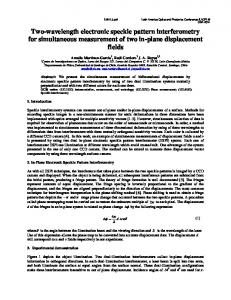
Fig. 2. Measurement results from using traditional phase-shifting technology. 50


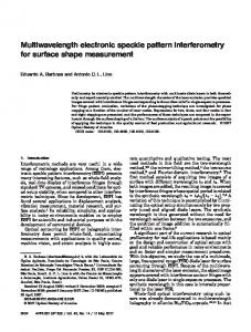
Fig. 3. Experimental results retrieved from the 共5,1兲 algorithm.

herein. Similar to the DC-共1,5兲 algorithm, the DC共5,1兲 algorithm performs the correlation calculation between the five intensity maps from the original state and the single intensity from the deformed state. The noise immunity of the direct-correlation algorithm can be maintained in this algorithm. In addition, the advantages of the 共5,1兲 algorithm such as its applicability for high-speed dynamic ESPI measurements are maintained as well. Starting from the intensity maps recorded before and after the specimen is deformed, i.e., I Ba ⫽ I 1 ⫹ I 2 ⫹ 2共I 1 I 2兲

1兾2

cos共⌽⬘ ⫺ ⌬⌽ ⫺ 2␤兲,

I Bb ⫽ I 1 ⫹ I 2 ⫹ 2共I 1 I 2兲

1兾2

cos共⌽⬘ ⫺ ⌬⌽ ⫺ ␤兲,

⌫ b⬘ ⫽ 12 关1 ⫹ cos共⌬⌽ ⫺ ␤兲兴, 1

⌫ c⬘ ⫽ 2 关1 ⫹ cos共⌬⌽兲兴, 1

⌫ d⬘ ⫽ 2 关1 ⫹ cos共⌬⌽ ⫹ ␤兲兴, 1

⌫ e⬘ ⫽ 2 关1 ⫹ cos共⌬⌽ ⫹ 2␤兲兴.

(30)

The phase difference ⌬⌽ can then be calculated by tan共⌬⌽兲 ⫽

关1 ⫺ cos共2␤兲兴共⌫ b⬘ ⫺ ⌫ d⬘兲 . sin共␤兲共2⌫ c⬘ ⫺ ⌫ a⬘ ⫺ ⌫ e⬘兲

(31)

I Bc ⫽ I 1 ⫹ I 2 ⫹ 2共I 1 I 2兲 1兾2 cos共⌽⬘ ⫺ ⌬⌽兲,

Implementing the above-mentioned phase-shifting14 and signal-processing algorithms for real experimental data is examined in Section 5.

I Bd ⫽ I 1 ⫹ I 2 ⫹ 2共I 1 I 2兲 1兾2 cos共⌽⬘ ⫺ ⌬⌽ ⫹ ␤兲,

5. Experimental Verification and Results

I Be ⫽ I 1 ⫹ I 2 ⫹ 2共I 1 I 2兲 1兾2 cos共⌽⬘ ⫺ ⌬⌽ ⫹ 2␤兲, I A ⫽ I 1 ⫹ I 2 ⫹ 2共I 1 I 2兲

1兾2

cos共⌽⬘兲,

(29)

we can rewrite the correlation coefficients for each phase-shifting step as ⌫ a⬘ ⫽ 12 关1 ⫹ cos共⌬⌽ ⫺ 2␤兲兴,

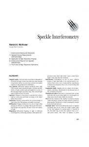
The optical setup used for the experimental verifications is shown in Fig. 1, which shows a typical ESPI setup, except for the configuration used to execute the phase-shifting operations. In a typical phaseshifting operation a mirror driven by some sort of actuator capable of inducing small displacement is used to induce the predesignated phase needed. 1 January 2002 兾 Vol. 41, No. 1 兾 APPLIED OPTICS

51

Fig. 4. Experimental results computed from the DC-共5,1兲 algorithm.

In the configuration shown in Fig. 1 a lead zirconate titanate, PZT, actuator from Tokin Corporation15,16 is attached to a fix end to drive a retroreflector to perform the phase-shifting procedures. The main advantage of the configuration shown is that the optical path does not change during the phase-shifting operation, which can significantly reduce efforts needed to set up the spatial filters typically used within the ESPI optical path. The phase obtained from this arrangement can be written as ⌬⌽ ⫽ 共K3 ⫺ K1兲䡠 L ⫽ 共V3 ⫺ V1兲䡠 L ⫽

⫽

2␲ ˆ ˆ ˆ ⫺ cos共45°兲Zˆ 兴其䡠关L XX 兵Z ⫺ 关sin共45°兲Y ␭ ˆ ⫹ L ZZˆ 兴 ⫹ L YY 2␲ 兵关1 ⫹ cos共45°兲兴 L Z ⫺ sin共45°兲 L Y其, ␭

(32)

where L is the displacement vector and LY and LZ are the displacements along the Y and the Z axes. This arrangement was used to perform a five-step phaseshifting algorithm to measure the displacement of an object under a point load. The phase maps from the undeformed and the deformed states, i.e., a total of 10 52


intensity maps, were recorded. These data were first computed by using both the 共5,1兲 and the 共1,5兲 algorithms to compare results generated by these two algorithms. Furthermore phase-unwrapping methods called the discrete cosine transform 共DCT) 共Ref. 9兲 and the discrete Fourier transform 共DFT兲共Ref. 14兲 were adopted for comparison purposes owing to their path independency and simplification. Some issues related to the domain of interest about DCT and DFT must be further explained owing to their behaviors at the boundaries.10,11,14 Considering the case that N ⫻ N sample points must be analyzed, a N ⫻ N matrix that represents the phase change induced by the displacement are to be obtained. The DCT algorithm can be executed across the N ⫻ N sample points directly. On the other hand, to use the DFT algorithm, the N ⫻ N data region must be expanded to 2N ⫻ 2N by taking the mirror reflection of the original N ⫻ N data points and then stitched back. More specifically, the concept of period normal equations and the selfrepeating behavior of the DFT would induce a jump on the boundary unless the methodology mentioned above was implemented. Furthermore, the fast Fourier transform 共FFT兲 was also adopted, because adopting DFT increases the number of data points that must be handled by a factor of 4. To meet the

need of FFT, the domain was further edited by adding zeros to change the 2N ⫻ 2N to 2m ⫻ 2m, where m is an exponent of a power of 2. It has long been known that the FFT runs more than 4 times faster than the data points to be handled. The results from using the traditional phase-shifting technology mentioned above are shown in Fig. 2. Figure 2共a兲 shows the phase map from the undeformed state computed by the traditional five-step phase-shifting technique. Figure 2共b兲 is the phase map of the deformed state computed by the five-step phase-shifting technique as well. Subtracting Fig. 2共b兲 from Fig. 2共a兲 generated the results shown in Fig. 2共c兲. Figure 2共d兲 is the phase-unwrapping results obtained from the DCT. The noisy and the cloudy results shown in Fig. 2 clearly reveal that the traditional phase-shifting technique is not adequate to handle such a noisy data set. The traditional technique not only requires a long measurement time but also generates unnecessary data sets. It is clear from the results above that the traditional phase-shifting approach is not suitable for noisy ESPI measurement data. Figure 3 was obtained by using the 共5,1兲 algorithm and the DCT phase-unwrapping algorithm to compute the same data set. Figure 3共a兲 is the phase map computed by the 共5,1兲 algorithm. Figure 3共b兲 is the unwrapped phase obtained by the DCT. Figure 3共c兲 is the three-dimensional plot of the data shown in Fig. 3共b兲. Because only a one phase-shifting procedure needs to be performed in the 共5,1兲 algorithm, the measurement time is significantly reduced. Note that more intensity maps usually introduce more noise due to an external disturbance such as air turbulence or outside vibration. The results from using the 共1,5兲 algorithm were found to be similar to those data in Fig. 3 and thus are not discussed here. A comparison of the results in Figs. 2 and 3 indicates that the quality of the phase-unwrapping result improves with adoption of the 共5,1兲 algorithm. Figure 4 shows the result from combining the 共5,1兲 algorithm and the direct-correlation algorithm, i.e., the DC-共5,1兲 algorithm. Figure 4共a兲 shows the wrapped phase map obtained with this integrated algorithm. Figure 4共b兲 shows the unwrapped phase computed from using the DCT, and Fig. 4共c兲 shows the three-dimensional plot of the data in Fig. 4共b兲. Again the results from using the DC-共1,5兲 algorithm are very similar to those data in Fig. 4. By comparing the results in Fig. 4 and those in Fig. 3, it is clear that the DC-共5,1兲 algorithm provides higher-quality ESPI phase maps than the 共5,1兲 algorithm. Note that the only disadvantage of the DC共5,1兲 algorithm when compared with the 共5,1兲 algorithm is the longer computation time needed because more tedious calculation steps must be performed to compute the correlation coefficients. 6. Conclusions and Discussions

To overcome some difficulties, such as long measurements, long computation time, and noisy or cloudy phase maps, in using a traditional phase-shifting technique for ESPI and the like, two new set of meth-

ods were developed. The first set of methods includes two similar algorithms, the 共5,1兲 algorithm and the 共1,5兲 algorithm. Both of these algorithms can reduce the phase-shifting steps needed in either the undeformed or the deformed state. Our experimental investigations indicate that these two approaches provide comparable experimental results. Nevertheless the 共5,1兲 algorithm appears to be more useful because a high-speed camera can be used to record the specimen ESPI intensity map while the specimen is undergoing deformation. This basic configuration extends the application range of the ESPI into a high-speed dynamic vibration regime. The two new approaches were created by integrating the direct-correlation algorithm with either the 共5,1兲 algorithm or the 共5,1兲 algorithm. Experimental results were also obtained to compare the effectiveness of all these newly developed signal-processing algorithms. It has been shown clearly that the 共5,1兲 algorithm can be executed faster than traditional approaches. In addition, owing to the generic features of the 共5,1兲 algorithm, this approach is suitable for high-speed dynamic deformation. To enhance further the effectiveness of the newly developed algorithms for ESPI applications, the 共5,1兲 algorithm was integrated with the direct-coefficient algorithm to form the DC-共5,1兲 algorithm. For noisy phase maps the ESPI experimental results processed from using this novel DC-共5,1兲 algorithm were clear and free from the noise-propagation problem. References and Notes 1. R. Jones and C. Wykes, Holographic and Speckle Interferometry 共Cambridge University, Cambridge, UK, 1983兲. 2. A. J. Moore and J. R. Tyrer, “Phase-stepped ESPI and moire interferometry for measuring the stress-intensity factor and J integral,” Exp. Mech. 35, 306 –314 共1995兲. 3. J. N. Butters and J. A. Leendertz, “A double exposure technique for speckle pattern interferometry,” J. Phys. E 4, 277– 279 共1971兲. 4. K. Creath, “Phase-shifting speckle interferometry,” Appl. Opt. 24, 3053–3058 共1985兲. 5. P. Hariharan, B. F. Orbel, and T. Eiju, “Digital phase-shifting interferometry: a simple error-compensating phase calculation,” Appl. Opt. 26, 2504 –2507 共1987兲. 6. D. R. Schmitt and R. W. Hunt, “Optimization of fringe pattern calculation with direct correlations in speckle interferometry,” Appl. Opt. 36, 8848 – 8857 共1997兲. 7. C. Gorecki, “Phase-correlation techniques for quasi-real-time measurement of deformations with digital speckle interferometry,” Appl. Opt. 33, 2933–2938 共1994兲. 8. J. Pomarico, R. Arizaga, R. Towoba, and H. Rabal, “Algorithm to compute spacing of digital speckle correlation fringes,” Optik 共Stuttgart兲 95, 125–127 共1993兲. 9. D. C. Ghiglia and L. A. Romero, “Robust two-dimensional weighted and unweighted phase unwrapping that uses fast transforms and iterative methods,” J. Opt. Soc. Am. A 11, 107–117 共1994兲. 10. H. Takajo and T. Takahashi, “Noniterative method for obtaining the exact solution for the normal equation in a leastsquares phase estimation,” J. Opt. Soc. Am. A 5, 1818 –1827 共1988兲. 11. H. Takajo and T. Takahashi, “Least-squares phase estimation from the phase difference,” J. Opt. Soc. Am. A 5, 416 – 425 共1988兲. 1 January 2002 兾 Vol. 41, No. 1 兾 APPLIED OPTICS

53

12. H. Y. Chang, C. W. Chen, C. K. Lee, and C. P. Hu, “The tapestry cellular automata phase unwrapping algorithm for nondestructive testing,” J. Opt. Lasers Eng. 30, 487–502 共1998兲. 13. C. W. Chen, H. Y. Chang, and C. K. Lee, “An innovative phase shifting system for nondestructive testing,” J. Chin. Soc. Appl. Mech. 14, 31–39 共1998兲. 14. Y. C. Chen, S. S. Lee, C. M. Lee, C. K. Lee, and G. B. Yeh, “New methodology for measuring highly aberrated wave fronts in-

54


duced by diffractive optical elements,” in Testing, Packaging, Reliability, and Applications of Semiconductor Lasers IV, M. Fallahi, J. Linden, and S. Wang, eds., Proc. SPIE 3626, 248 – 259 共1999兲. 15. S. Takahashi, “Multilayer piezoelectric ceramics actuators and their applications,” Jpn. J. Appl Phys. 24, 41– 45 共1985兲. 16. Tokin America Inc., “Multilayer piezoelectric actuator,” Insp. Rec. 912-46S-02039, displacement: 14.4 ␮m at 100 V dc for 17.981-mm length 共1991兲.