PHD THESIS Complex Wavelet Transform: application to denoising

POLITEHNICA UNIVERSITY OF TIMISOARA UNIVERSITÉ DE RENNES 1

PHD THESIS to obtain the title of

PhD of Science of the Politehnica University of Timisoara and Université de Rennes 1

Defended by

Ioana Adam

Complex Wavelet Transform: application to denoising

Thesis Advisors : Alexandru Isar Jean-Marc Boucher

Contents 1 Introduction 1.1 Motivation . . . . . . . . . . . . . . . . . . . . . . . . . . . . . . . . . . . 1.2 Thesis outline . . . . . . . . . . . . . . . . . . . . . . . . . . . . . . . . .

1 1 2

2 Wavelet Transforms 2.1 Introduction . . . . . . . . . . . . . . . . . . . . . . . . . . . . . . . . . . 2.1.1 Wavelet Definition . . . . . . . . . . . . . . . . . . . . . . . . . . 2.1.2 Wavelet Characteristics . . . . . . . . . . . . . . . . . . . . . . . . 2.1.3 Wavelet Analysis . . . . . . . . . . . . . . . . . . . . . . . . . . . 2.1.4 Wavelet History . . . . . . . . . . . . . . . . . . . . . . . . . . . . 2.1.5 Wavelet Terminology . . . . . . . . . . . . . . . . . . . . . . . . . 2.2 Evolution of Wavelet Transform . . . . . . . . . . . . . . . . . . . . . . . 2.2.1 Fourier Transform (FT) . . . . . . . . . . . . . . . . . . . . . . . 2.2.2 Short Time Fourier Transform (STFT) . . . . . . . . . . . . . . . 2.2.3 Wavelet Transform (WT) . . . . . . . . . . . . . . . . . . . . . . 2.2.4 Comparative Visualization . . . . . . . . . . . . . . . . . . . . . . 2.3 Theoretical Aspects of Wavelet Transform . . . . . . . . . . . . . . . . . 2.3.1 Continuous Wavelet Transform (CoWT) . . . . . . . . . . . . . . 2.3.2 Discrete Wavelet Transform (DWT) . . . . . . . . . . . . . . . . . 2.4 Implementation of DWT . . . . . . . . . . . . . . . . . . . . . . . . . . . 2.4.1 Multiresolution Analysis (MRA) . . . . . . . . . . . . . . . . . . . 2.4.2 Filter-bank Implementation of the Discrete Wavelet Transform . . 2.4.3 Perfect Reconstruction . . . . . . . . . . . . . . . . . . . . . . . . 2.5 Extensions of DWT . . . . . . . . . . . . . . . . . . . . . . . . . . . . . . 2.5.1 Two Dimensional DWT (2D DWT) . . . . . . . . . . . . . . . . . 2.5.2 Wavelet Packet Transform . . . . . . . . . . . . . . . . . . . . . . 2.5.2.1 One-Dimensional Wavelet Packet Transform (1D WPT) 2.5.2.2 Two-Dimensional Wavelet Packet Transform (2D WPT) 2.5.3 Undecimated Discrete Wavelet Transform (UDWT) . . . . . . . . 2.6 Applications of Wavelet Transforms . . . . . . . . . . . . . . . . . . . . . 2.7 Limitations of Wavelet Transforms . . . . . . . . . . . . . . . . . . . . . 2.7.1 Shift Sensitivity . . . . . . . . . . . . . . . . . . . . . . . . . . . . 2.7.2 Directional selectivity . . . . . . . . . . . . . . . . . . . . . . . . . 2.8 Summary . . . . . . . . . . . . . . . . . . . . . . . . . . . . . . . . . . .

3 3 3 3 4 4 4 5 5 6 6 7 8 8 9 11 11 13 17 18 18 22 22 26 28 30 31 31 32 33

i

CONTENTS

ii

3 Complex Wavelet Transforms (CWT) 3.1 Introduction . . . . . . . . . . . . . . . . . . . . . . . . . . . . . . 3.2 Earlier Work . . . . . . . . . . . . . . . . . . . . . . . . . . . . . . 3.3 Recent Developments . . . . . . . . . . . . . . . . . . . . . . . . . 3.4 Examples of Complex Wavelet Transforms . . . . . . . . . . . . . 3.4.1 Dual-Tree based Complex Wavelet Transforms . . . . . . . 3.4.1.1 One-dimensional DT CWT . . . . . . . . . . . . 3.4.1.2 Two-dimensional DT CWT . . . . . . . . . . . . 3.4.2 Projection-based CWTs . . . . . . . . . . . . . . . . . . . 3.4.3 Hyperanalytic Wavelet Transform . . . . . . . . . . . . . . 3.4.3.1 Analytical Discrete Wavelet Transform (ADWT) 3.4.3.2 Hyperanalytic Wavelet Transform (HWT) . . . . 3.5 Advantages and Applications of Complex Wavelet Transforms . . 3.6 Summary . . . . . . . . . . . . . . . . . . . . . . . . . . . . . . .

. . . . . . . . . . . . .

. . . . . . . . . . . . .

. . . . . . . . . . . . .

. . . . . . . . . . . . .

35 35 35 39 40 40 41 42 46 50 50 56 59 61

4 Denoising 4.1 Introduction . . . . . . . . . . . . . . . . . . . . . . . . . . . . . . . . . . 4.1.1 Digital images and noise . . . . . . . . . . . . . . . . . . . . . . . 4.1.2 Denoising algorithms . . . . . . . . . . . . . . . . . . . . . . . . . 4.1.3 Local averaging and PDEs . . . . . . . . . . . . . . . . . . . . . . 4.1.4 The total variation minimization . . . . . . . . . . . . . . . . . . 4.1.5 Properties of natural images . . . . . . . . . . . . . . . . . . . . . 4.1.6 Frequency domain filters . . . . . . . . . . . . . . . . . . . . . . . 4.1.7 Non local averaging . . . . . . . . . . . . . . . . . . . . . . . . . . 4.2 Non-parametric Denoising . . . . . . . . . . . . . . . . . . . . . . . . . . 4.2.1 Basic Concept . . . . . . . . . . . . . . . . . . . . . . . . . . . . . 4.2.2 Shrinkage Strategies . . . . . . . . . . . . . . . . . . . . . . . . . 4.2.2.1 A New Class of Shrinkage Functions Based on Sigmoid . 4.2.2.2 Translation invariant wavelet thresholding . . . . . . . . 4.2.2.3 A semi parametric denoising method using a MMSE estimator . . . . . . . . . . . . . . . . . . . . . . . . . . . . 4.3 Parametric Denoising . . . . . . . . . . . . . . . . . . . . . . . . . . . . . 4.3.1 The Bayesian Approach . . . . . . . . . . . . . . . . . . . . . . . 4.3.1.1 The Wiener Filter . . . . . . . . . . . . . . . . . . . . . 4.3.1.2 The adaptive soft-thresholding filter . . . . . . . . . . . 4.3.1.3 Local vs global . . . . . . . . . . . . . . . . . . . . . . . 4.3.1.4 Inter-scale dependency . . . . . . . . . . . . . . . . . . . 4.3.1.5 The Bishrink Filter . . . . . . . . . . . . . . . . . . . . . 4.3.1.6 Other statistical models for the wavelet coefficients . . . 4.4 Summary . . . . . . . . . . . . . . . . . . . . . . . . . . . . . . . . . . .

75 76 76 78 82 87 87 93 109 114

5 Speckle Reduction 5.1 Introduction . . . . . . . . . . . . . . . . 5.1.1 Speckle’s Statistics . . . . . . . . 5.1.2 Speckle Filtering Techniques . . . 5.1.2.1 Homomorphic Filtering

115 115 116 116 116

. . . .

. . . .

. . . .

. . . .

. . . .

. . . .

. . . .

. . . .

. . . .

. . . .

. . . .

. . . .

. . . .

. . . .

. . . .

. . . .

. . . .

. . . .

63 63 63 64 65 66 66 68 69 70 70 71 73 75

CONTENTS

5.2

5.3

5.4

5.1.2.2 Pixel-ratioing - based filtering . . . . . . . 5.1.3 Quality measures . . . . . . . . . . . . . . . . . . . Spatial-domain Speckle reduction methods . . . . . . . . . 5.2.1 Frost Filter . . . . . . . . . . . . . . . . . . . . . . 5.2.2 Kuan Filter . . . . . . . . . . . . . . . . . . . . . . 5.2.3 Lee Filter . . . . . . . . . . . . . . . . . . . . . . . 5.2.4 Other speckle reduction filters in the spatial domain 5.2.4.1 Zero-order Wiener filter . . . . . . . . . . 5.2.4.2 A MAP filter acting in the spatial domain 5.2.4.3 Model-Based Despeckling (MBD) . . . . . Speckle reduction in the wavelet domain . . . . . . . . . . 5.3.1 Non-parametric filters . . . . . . . . . . . . . . . . 5.3.2 MAP filters . . . . . . . . . . . . . . . . . . . . . . 5.3.2.1 MAP filters associated with 2D UDWT . 5.3.2.2 MAP filters associated with 2D DWT . . 5.3.2.3 MAP filters associated with 2D DTCWT . 5.3.2.4 MAP filters associated with HWT . . . . Summary . . . . . . . . . . . . . . . . . . . . . . . . . . .

iii . . . . . . . . . . . . . . . . . .

. . . . . . . . . . . . . . . . . .

. . . . . . . . . . . . . . . . . .

. . . . . . . . . . . . . . . . . .

. . . . . . . . . . . . . . . . . .

. . . . . . . . . . . . . . . . . .

. . . . . . . . . . . . . . . . . .

. . . . . . . . . . . . . . . . . .

118 118 118 119 120 120 121 121 122 122 124 124 125 125 128 130 137 140

6 Conclusions 145 6.1 Contributions . . . . . . . . . . . . . . . . . . . . . . . . . . . . . . . . . 145 6.2 Perspectives . . . . . . . . . . . . . . . . . . . . . . . . . . . . . . . . . . 146

List of Figures 2.1 2.2 2.3 2.4 2.5 2.6 2.7 2.8 2.9 2.10 2.11 2.12 2.13 2.14 2.15 2.16 2.17 2.18 2.19 2.20 2.21 2.22 2.23 2.24 2.25 2.26 2.27 2.28 3.1 3.2 3.3 3.4

Wavelet . . . . . . . . . . . . . . . . . . . . . . . . . . . . . . . . . . . . Time-frequency representation of the Fourier Transform. . . . . . . . . . Time-frequency representation of the Short Time Fourier Transform . . . Time-frequency representation of the Wavelet Transform. . . . . . . . . . Approximation Spaces (Vj ) and Detail Spaces (Wj ) . . . . . . . . . . . . One-level DWT decomposition scheme . . . . . . . . . . . . . . . . . . . DWT decomposition tree . . . . . . . . . . . . . . . . . . . . . . . . . . . One-level DWT reconstruction scheme . . . . . . . . . . . . . . . . . . . Three-level DWT reconstruction scheme . . . . . . . . . . . . . . . . . . One-level 2D DWT decomposition scheme . . . . . . . . . . . . . . . . . 2D DWT coefficients’ image . . . . . . . . . . . . . . . . . . . . . . . . . Example of a 2D DWT decomposition . . . . . . . . . . . . . . . . . . . One-level 2D DWT reconstruction scheme . . . . . . . . . . . . . . . . . Binary tree of wavelet packet spaces . . . . . . . . . . . . . . . . . . . . . Example of admissible wavelet packet binary tree . . . . . . . . . . . . . One-dimensional Wavelet Packet Decomposition . . . . . . . . . . . . . . One-dimensional Wavelet Packet Reconstruction . . . . . . . . . . . . . . Example of a wavelet packet quad-tree . . . . . . . . . . . . . . . . . . . One Level 2D WPT Decomposition Scheme . . . . . . . . . . . . . . . . One Level 2D WPT Reconstruction Scheme . . . . . . . . . . . . . . . . Three-Level UDWT Decomposition Scheme . . . . . . . . . . . . . . . . Relation between the filters corresponding to two consecutive levels of UDWT decomposition . . . . . . . . . . . . . . . . . . . . . . . . . . . . Three-Level UDWT Reconstruction Scheme . . . . . . . . . . . . . . . . Relation between the filters corresponding to two consecutive levels of UDWT reconstruction . . . . . . . . . . . . . . . . . . . . . . . . . . . . One Level 2D UDWT Decomposition Scheme . . . . . . . . . . . . . . . One Level 2D UDWT Reconstruction Scheme . . . . . . . . . . . . . . . Shift-sensitivity . . . . . . . . . . . . . . . . . . . . . . . . . . . . . . . . DWT’s Directional selectivity . . . . . . . . . . . . . . . . . . . . . . . . Complex wavelet tree . . . . . . . . . . . . . . . . . . . . . . . . 2-D Complex wavelet tree . . . . . . . . . . . . . . . . . . . . . Implementation of an analytical DWT . . . . . . . . . . . . . . The Q-shift version of the DT CWT, giving real and imaginary complex coefficients from tree a and tree b respectively. . . . . . iv

. . . . . . . . . . . . . . . parts of . . . . .

3 7 8 8 12 16 16 18 18 21 21 22 22 24 24 26 26 27 28 28 29 29 29 30 30 30 32 33 36 37 40 42

LIST OF FIGURES 3.5 3.6 3.7

3.8

3.9 3.10 3.11 3.12 3.13 3.14 3.15 3.16 3.17 3.18 3.19

3.20 3.21 3.22 3.23

3.24

4.1 4.2 4.3 4.4

4.5

Detail and approximation components at levels 1 to 4 of 16 shifted step responses of the DT CWT (a) and real DWT (b) . . . . . . . . . . . . . Input image used for the 2D shift sensitivity test . . . . . . . . . . . . . . Wavelet and scaling function components at levels 1 to 4 of an image using the 2D DT CWT (upper row) and 2D DWT (lower row). Only half of each wavelet image is shown in order to save space. . . . . . . . . . . . . . . . Basis functions of 2D Q-shift complex wavelets (top) and 2D real wavelet filters (bottom), all illustrated at level 4 of the transforms. The complex wavelets provide 6 directionally selective filters, while real wavelets provide 3 filters, only two of which have a dominant direction . . . . . . . . . . . Components from each subband of the reconstructed output image for a 4-level 2D DT CWT decomposition of Lena (central part (128x128) only) Projection-based CWT and its inverse . . . . . . . . . . . . . . . . . . . |H + (ω)|, the magnitude response of the mapping filter h+ . . . . . . . . Relationship between L2 (R), Hardy-space and Softy-space . . . . . . . . PCWT . . . . . . . . . . . . . . . . . . . . . . . . . . . . . . . . . . . . . Non-redundant mapping . . . . . . . . . . . . . . . . . . . . . . . . . . . Equivalent implementations of the ADWT . . . . . . . . . . . . . . . . . The implementation of the Hilbert transformer . . . . . . . . . . . . . . . The use of the Hilbert transform in simulations . . . . . . . . . . . . . . A visual comparison ment to illustrate the shiftability of ADWT, DT CWT and DWT . . . . . . . . . . . . . . . . . . . . . . . . . . . . . . . . . . . The system used for the shift-invariance analysis of the third level of the wavelet decomposition. In this example is considered the case of the proposed implementation of ADWT . . . . . . . . . . . . . . . . . . . . . . . The dependency of the degree of shift-invariance of HWT on the regularity of the mother wavelet used for its computation . . . . . . . . . . . . . . . HWT implementation scheme . . . . . . . . . . . . . . . . . . . . . . . . Comparison in the 2D case between the HWT, the DT CWT and the DWT The strategy of directional selectivity enhancement in the HH subband illustrated through the transfer functions of the systems used in the HWT implementation . . . . . . . . . . . . . . . . . . . . . . . . . . . . . . . . The absolute values of the spectra of horizontal and diagonal detail subimages obtained after the first iterations of 2D DWT and HWT. In the HWT case, the real and imaginary parts of complex coefficients are separated Examples of standard WaveShrink functions . . . . . . . . . . . . . . . . Denoising scheme using HWT and Zero-Order Wiener filter . . . . . . . . The architecture of HWT with directional selectivity enhancement . . . . The histograms of some subbands of the HWT of the image Lena computed using the mother wavelets ‘Daub, 20’ are represented semi logarithmically (on the vertical axis are represented the logarithms of the values of the histograms) in blue. The corresponding linear dependencies are represented in red. . . . . . . . . . . . . . . . . . . . . . . . . . . . . . . . . . . . . . Different types of wavelet coefficients’ dependencies . . . . . . . . . . . .

v

43 45

46

47 48 48 49 49 50 50 51 52 52 53

54 55 57 58

59

60 74 83 84

85 88

LIST OF FIGURES 4.6

4.7 4.8 4.9 4.10

4.11

4.12

4.13 4.14 4.15

From left to right and up to bottom: original Barbara image; the image of local variances, the correspondent classes (obtained comparing the local variances with decreasing thresholds) - the first four classes contain textures and contours; the last two classes contain textures and homogeneous regions. For each of the last six pictures, the pixels belonging to a different class are represented in yellow. . . . . . . . . . . . . . . . . . . . . . . . . The architecture of the denoising system based on the association of the DE DWT with the bishrink filter . . . . . . . . . . . . . . . . . . . . . . A comparison of the directional selectivity of 2D DWT (a) and HWT (b). The architecture of the denoising system based on the association of the DE HWT with the bishrink filter . . . . . . . . . . . . . . . . . . . . . . A first implementation of the new synthesis mechanism. It can be applied to the association of the real and imaginary parts of the HWT coefficients or of their magnitudes with the bishrink filter . . . . . . . . . . . . . . . The final implementation of the new synthesis mechanism. It can be applied to the association of the real and imaginary parts of the HWT coefficients or of their magnitudes with the bishrink filter . . . . . . . . . . . A comparison between the results obtained using the association real and imaginary parts of HWT - bishrink (up) and the denoising method proposed in this section (bottom), for the image Lena perturbed by AWGN with σn = 35 . . . . . . . . . . . . . . . . . . . . . . . . . . . . . . . . . The architecture of the fusion system in the interior of one of the classes C6 − C9 from the system with the architecture in figure 4.11. . . . . . . . Directional elliptic windows . . . . . . . . . . . . . . . . . . . . . . . . . Simulation results using both directional and square estimation windows

The architecture of homomorphic filtering system. The mean correction mechanism and the kernel are highlighted. . . . . . . . . . . . . . . . . . 5.2 Test image . . . . . . . . . . . . . . . . . . . . . . . . . . . . . . . . . . . 5.3 The image in figure 5.2 having a number of looks equal to 1 treated with a Frost filter using a rectangular moving window of size 7x7. . . . . . . . 5.4 The image in figure 5.2 having a number of looks equal to 1 treated with a Kuan filter using a rectangular moving window of size 7x7. . . . . . . . 5.5 The image in figure 5.2 having a number of looks equal to 1 treated with a Lee filter using a rectangular moving window of size 7x7. . . . . . . . . 5.6 The image in figure 5.2 treated with a zero-order Wiener filter. . . . . . . 5.7 Model-Based Despecking simulation results. . . . . . . . . . . . . . . . . 5.8 A SAR image denoising system based on the association of the DE DWT with the Soft-thresholding filter . . . . . . . . . . . . . . . . . . . . . . . 5.9 The output of the system in figure 5.8 when at its input is applied the image in figure 5.2. . . . . . . . . . . . . . . . . . . . . . . . . . . . . . . 5.10 A comparison of the results obtained despeckling the image (a) with the algorithm proposed in [GD06] (b) and with the MBD algorithm proposed in [WD00] (c). . . . . . . . . . . . . . . . . . . . . . . . . . . . . . . . . .

vi

96 98 99 100

102

103

104 105 107 108

5.1

117 119 119 120 121 121 122 124 125

130

LIST OF FIGURES

vii

5.11 The result reported in [IIM+ 05]. The noisy image was acquired by IFREMER, Brest, France (ENL = 7.34 - up). The denoised image (ENL = 76.64 - down) . . . . . . . . . . . . . . . . . . . . . . . . . . . . . . . . . 132 5.12 The architecture of the additive noise denoising kernel proposed in [IMI09]. 133 5.13 Synthesized speckle noise. First line, from left to right: clean image; synthesized speckle; noisy image (PSNR=21.4 dB). Second line, from left to right: denoised image (PSNR=31.4 dB); method noise; histograms of the noise (up) and method noise (bottom). . . . . . . . . . . . . . . . . . . . 134 5.14 From up to bottom: noisy sub-images; results obtained in [WD00]; results obtained applying the method proposed in [FA05]; results of the denoising method proposed in [IMI09]. . . . . . . . . . . . . . . . . . . . . . . . . . 135 5.15 Speckle removal for the sea-bed SONAR Swansea image (acquired by GESMA). Left: acquired image (ENL=3.4), Middle: result in [IIQ07] (ENL=106), Right: result of the denoising method proposed in [IMI09] (ENL=101.8). . . . . . . . . . . . . . . . . . . . . . . . . . . . . . . . . . 136 5.16 HWT - Adaptive soft-thresholding denoising results applied on Lena affected by multiplicative noise . . . . . . . . . . . . . . . . . . . . . . . . 138 5.17 HWT - Bishrink denoising results applied on Lena affected by multiplicative noise . . . . . . . . . . . . . . . . . . . . . . . . . . . . . . . . . . . 139 5.18 HWT + Bishrink vs. UDWT + GGPDF-based MAP . . . . . . . . . . . 140 5.19 HWT - Bishrink denoising results obtained for the test image . . . . . . 141 5.20 HWT - Bishrink denoising results applied on SONAR image. In this case the ENL is 50 times higher, while in the results presented in 5.15 is only about 30 times higher . . . . . . . . . . . . . . . . . . . . . . . . . . . . . 142 5.21 Results of HWT - Bishrink denoising applied on SAR image . . . . . . . 143

List of Tables 3.1 3.2

A comparison between two quasi shift-invariant WTs, the ADWT and the CS . . . . . . . . . . . . . . . . . . . . . . . . . . . . . . . . . . . . . . . A comparison of ADWT, DT CWT and DWT . . . . . . . . . . . . . . .

PSNRs obtained using the soft-thresholding filter in the 2D DWTs domain, computed using the mother wavelets from the Daubechies family and in the DE DWT domain, for the image Lena perturbed with AWGN with different variances . . . . . . . . . . . . . . . . . . . . . . . . . . . . . . . 4.2 PSNRs obtained using the hard-thresholding filter in the 2D DWTs domain, computed using the mother wavelets from the Daubechies family and in the DE DWT domain, for the image Lena perturbed with AWGN with different variances . . . . . . . . . . . . . . . . . . . . . . . . . . . . 4.3 Denoising using zero-order Wiener filter directly on the image . . . . . . 4.4 Denoising using zero-order Wiener filters, both global and local, in the 2D DWT domain . . . . . . . . . . . . . . . . . . . . . . . . . . . . . . . . . 4.5 Denoising using zero-order local Wiener filter, in the HWT domain . . . 4.6 A comparison of the results obtained with the associations HWT-adaptive stf and HWT-local zero order Wiener filter used to denoise the image Lena perturbed with AWGN with different variances . . . . . . . . . . . . . . 4.7 PSNRs obtained using the bishrink filter in the 2D DWTs domain, computed using the mother wavelets from the Daubechies family and in the DE DWT domain, for the image Lena perturbed with AWGN with different variances . . . . . . . . . . . . . . . . . . . . . . . . . . . . . . . . . . . . 4.8 A comparison of the performance obtained associating the bishrink filter with the DWT and with the HWT respectively for denoising the image Lena perturbed with AWGN with different variances. The mother wavelets ‘Daub,20’ was used in both experiments. . . . . . . . . . . . . . . . . . . 4.9 A comparison of the performance obtained associating the bishrink filter with the real and imaginary parts of HWT and with the magnitude of the HWT respectively for denoising the image Lena perturbed with AWGN with different variances. The mother wavelets ‘Daub,20’ was used in both experiments. . . . . . . . . . . . . . . . . . . . . . . . . . . . . . . . . . . 4.10 The results obtained associating the bishrink filter with the real and imaginary parts of HWT and DEHWT for denoising the image Lena perturbed by AWGN with different variances. The mother wavelets: ‘Daub,4’ ‘Daub,20’ were used. . . . . . . . . . . . . . . . . . . . . . . . . . . . . .

55 56

4.1

viii

72

73 81 82 83

87

98

99

100

101

LIST OF TABLES 4.11 Results obtained applying the architecture in figure 4.9 where the magnitudes of HWTs are associated to the bishrink filter to the Lena image perturbed by AWGN with different variances. . . . . . . . . . . . . . . . 4.12 Results obtained applying the new synthesis mechanism. . . . . . . . . . 4.13 Contour errors obtained by applying the new synthesis mechanism. . . . 4.14 Results obtained applying the bishrink filter in association with HWT with ‘Daub,6’ and ‘Daub,20’, respectively with HWT DE, using directional estimation windows . . . . . . . . . . . . . . . . . . . . . . . . . . . . . . 4.15 Contour errors obtained by applying the bishrink filter in association with HWT with Daub,6 and HWT DE, using directional estimation windows . 4.16 Comparison HWT - bishrink vs. those reported in [Shu05] . . . . . . . . 5.1 5.2 5.3

5.4 5.5

5.6 5.7 5.8

ix

101 106 106

107 108 109

Comparison of the performances of some classical speckle reduction systems120 A comparison of different spatial-domain speckle reduction methods, from the S/MSE point of view. . . . . . . . . . . . . . . . . . . . . . . . . . . 122 A comparison of the ENLs of three regions of a SAR image obtained using the denoising method proposed in [FBB01] with ENLs of the same regions obtained using the association of the 2D UDWT with the Gamma-MAP filter which includes an edge detector inside each estimation window. . . 126 PSNR performances of the proposed despeckling algorithm applied to noisy versions of ‘Lena’ image. . . . . . . . . . . . . . . . . . . . . . . . . . . . 127 A comparison of the performance of the homomorphic Γ-WMAP filter (which acts in the 2D UDWT domain) with the performance of the ΓMAP filter (which acts in the spatial domain) for three analyzing window sizes, in terms of ENL. . . . . . . . . . . . . . . . . . . . . . . . . . . . . 128 PSNR performances of HWT associated with adaptive soft-thresholding, applied to noisy versions of ‘Lena’ image . . . . . . . . . . . . . . . . . . 137 PSNR performances of HWT, respectively HWTDE, associated with bishrink, applied to noisy versions of ‘Lena’ image. . . . . . . . . . . . . 139 HWT + Bishrink vs. UDWT + GGPDF-based MAP from the PSNR point of view . . . . . . . . . . . . . . . . . . . . . . . . . . . . . . . . . 140

Chapter 1 Introduction The introductory chapter presents the motivation of the work and ends with a short outline of the thesis.

1.1

Motivation

Wavelet theory is one of the most modern areas of mathematics. Masterfully developed by French researchers, such as Yves Meyer, Stéphane Mallat and Albert Cohen, this theory, is now used as an analytical tool in most areas of technical research: mechanical, electronics, communications, computers, biology and medicine, astronomy an so on. In the field of signal and image processing, the main applications of wavelet theory are compression and denoising. In the context of denoising, the success of techniques based on the wavelet theory is ensured by the ability of decorrelation (separation of noise and useful signal) of the different discrete wavelet transforms [FBB01, ICN02]. Because the signal is contained in a small number of coefficients of such a transform, all other coefficients essentially contain noise. By filtering these coefficients, most of the noise is eliminated. Thus, each method of image denoising based on the use of wavelets follows the classic method, in three steps: computing a discrete wavelet transform of the image to be denoised, filtering in the wavelet domain and the computation of the corresponding inverse wavelet transform. Throughout recent years, many wavelet transforms (WT) have been used to operate denoising. The first one was the discrete wavelet transform, [DJ94]. It has three main disadvantages [Kin01]: lack of shift invariance, lack of symmetry of the mother wavelet and poor directional selectivity. These disadvantages can be diminished using a complex wavelet transform [Kin01, Kin00]. More than 20 years ago, Grossman and Morlet [GM84] developed the continuous wavelet transform [SBK05]. A revival of interest in later years has occurred in both signal processing and statistics for the use of complex wavelets [BN04], and complex analytic wavelets, particularly in [Kin99, Sel01]. It may be linked to the development of complex-valued discrete wavelet filters [LM95] and the clever dual filter bank [Kin99, SBK05]. The complex WT has been shown to provide a powerful tool in signal and image analysis [Mal99]. In [OM06], the authors derived large classes of wavelets generalizing the concept of 1-D local complex-valued analytic decomposition introducing 2-D vector-valued hyperanalytic decomposition. 1

1.2. Thesis outline

2

The present work is situated in this context, and, by introducing a new version of the Hyperanalytic Wavelet Transform and by combining this transform with various parametric and non-parametric filtering techniques attempts to provide a solution to the denoising problem. The new transform, by allowing the use of all the mother wavelet families that are usually used with the discrete wavelet transform, while achieving the desirable properties of complex wavelet transforms, such as quasi shift-invariance and a good directional selectivity, in association with different filters selected has provided good denoising results both when applied to images affected by additive noise or by multiplicative noise, as is the case of SAR images.

1.2

Thesis outline

The current thesis is organized as follows: • Chapter 1, Introduction, is made of a short presentation of the context the present work relies in, and an overview of the structure of the thesis. • Chapter 2, Wavelet Transforms, introduces the discrete wavelet transform (onedimensional and two-dimensional), the undecimated wavelet transform and the wavelet packet transform (one-dimensional and two-dimensional), explaining the concept of multiresolution analysis and the limitations of the discrete wavelet transform (shift sensitivity, reduced directional selectivity). • Chapter 3, Complex Wavelet Transforms, constitutes a sequel of the previous chapter by introducing the complex wavelet transforms. The Hyperanalytic Wavelet Transform (HWT) is introduced, this representing the thesis’ main contribution and a parallel is drawn between this transform and the dual-tree complex wavelet transform, DTCWT. A special attention is given to the quasi shift-invariance and to the good directional selectivity of the HWT. • Chapter 4, Denoising, is a thorough presentation of denoising. The noise is considered to be additive in this case. The wavelet-based denoising techniques are emphasized. A distinction is being made between the non-parametric and parametric methods, emphasizing the second category. I have insisted on the maximum a posteriori (MAP) parametric methods. The importance of the coefficients’ interscale dependency is highlighted. Starting from the Gaussian mixture model for characterizing different scales (GSM), the bishrink filter is introduced. The association of the HWT with the bishrink filter is studied and compared with the denoising performances of other methods. • Chapter 5, Speckle Reduction, is a continuation of chapter 4 and its goal is the reduction of multiplicative speckle-type noise, affecting the SAR and SONAR images. I have developed a homomorphic denoising method based on the association of the HWT with the bishrink filter. This method is then compared with the classical despecklisation methods and with other methods proposed in the literature. • Chapter 6, Conclusions, presents the conclusions drawn and future perspectives.

Chapter 2 Wavelet Transforms 2.1 2.1.1

Introduction Wavelet Definition

The term ‘wavelet’ refers to an oscillatory vanishing wave with time-limited extend, which has the ability to describe the time-frequency plane, with atoms of different time supports (see fig. 2.1). Generally, wavelets are purposefully crafted to have specific properties that make them useful for signal processing. They represent a suitable tool for the analysis of non-stationary or transient phenomena.

Figure 2.1: Wavelet

2.1.2

Wavelet Characteristics

Wavelets are a mathematical tool, that can be used to extract information from many kinds of data, including audio signals and images. Mathematically, the wavelet ψ, is a function of zero average, having the energy concentrated in time: Z ∞ ψ (t) dt = 0, (2.1) −∞

3

2.1. Introduction

4

In order to be more flexible in extracting time and frequency informations, a family of wavelets can be constructed from a function ψ (t), also known as the ‘Mother Wavelet’, which is confined in a finite interval. ‘Daughter Wavelets’, ψu,s (t) are then formed by translation with a factor u and dilation with a scale parameter s: 1 t−u ψu,s (t) = √ · ψ (2.2) s s

2.1.3

Wavelet Analysis

The wavelet analysis is performed by projecting the signal to be analyzed on the wavelet function. It implies a multiplication and an integration: Z hx (t) , ψu,s (t)i = x (t) ψu,s (t) dt. Depending on the signal characteristics that we want to analyze, we can use different scales and translations of the mother wavelet. The particularity of the wavelet analysis is that it allows us to change freely the size of the analysis function (window), to make it suitable for the needed resolution, in time or frequency domain. For high resolution in time-domain analysis we want to ‘capture’ all the sudden changes that appear in the signal, and we do that by using a contracted version of the mother wavelet. Conversely, for high-resolution in the frequency-domain we will be using a dilated version of the same function.

2.1.4

Wavelet History

The development of wavelets can be linked to several works in different domains, starting with the first wavelet introduced by Haar in 1909. In 1946, Denis Gabor, introduced the Gabor atoms or Gabor functions, which are functions used in analysis, a family of functions being built from translations and modulations of a generating function. In 1975, George Zweig, former particle physicist who had turned to neurobiology, has discovered the continuous wavelet transform (named first the cochlear transform and discovered while studying the reaction of the ear to sound). Morlet, studying reflection seismology observed that, instead of emitting pulses of equal duration, shorter waveforms at high frequencies should perform better in separating the returns of fine closely-spaced layers. Grossmann, who was working in theoretical physics, recognised in Morlet’s approach some ideas that were close to his own work on coherent quantum states. In 1982, Grossmann and Morlet have given the formulation of the Continuous Wavelet Transform. Yves Meyer recognized the importance of this fundamental mathematical tool and developed this theory with collaborators as Ingrid Daubechies (who introduced the orthogonal wavelets with compact support (1988) [Dau88]) and Stéphane Mallat (who proposed the filter-bank implementation scheme of the Discrete Wavelet Transform).

2.1.5

Wavelet Terminology

Due to Mallat’s implementation of the Wavelet transform, the filter-bank theory is closely related to the wavelet theory. Also, the concept of ‘Multiresolution Analysis’ (MRA) is

2.2. Evolution of Wavelet Transform

5

connected to the wavelet theory. Besides the classic wavelet transforms (Continuous Wavelet Transform and Discrete Wavelet Transform) we have more ‘evolved’ transforms connected with the wavelet theory, such as the Complex Wavelet Transform and the Wavelet Packets Transform.

2.2

Evolution of Wavelet Transform

For many years, classical signal processing was concentrated on the characterization of signals and on the designing of time-invariant and space-invariant operators that modify stationary signal properties. But the biggest amount of information is concentrated in the transients rather than in stationary signals. In the following, the evolution of the Wavelet transform will be described, having as departure point the Fourier Transform.

2.2.1

Fourier Transform (FT)

In the first part of the 19th century, Joseph Fourier, a French mathematician and physicist, showed that any periodic function can be decomposed in a series of simple oscillating functions, namely sines and cosines (or complex exponentials). The generalization to the non-periodic signals has come only a century later, and took the name of Fourier Transform (FT), a tribute brought to the original idea. The FT decomposes a signal in complex exponential functions at different frequencies. The equations used in the decomposition and reconstruction part are the following: Z ∞ X (ω) = x (t) · e−jωt dt, (2.3) −∞ Z ∞ 1 x (t) = X (ω) · ejωt dω. (2.4) 2π −∞ In the above equations, t stands for time, ω = 2πf for frequency, x denotes the signal in the time domain and X denotes the signal in the frequency domain (also known as the spectrum of the original signal). As can be seen from eq. 2.3, the computation of the FT is done over all times, making no distinction between signals’ stationary parts and transient ones (whether the frequency component ‘ω’ appears at time t1 or t2 , it will have the same effect at the output of the integration). The scaling property of the FT states that if we have a scaled version of the original xs (t): xs (t) = x (st) ,

(2.5)

then, its corresponding FT will be Xs (ω): 1 ω X . (2.6) |s| s We can observe from the last two equations that if we reduce the time spread of x by s (if s>1) than the FT is dilated by s, meaning that if what we have gained in time localization, we have lost in frequency localization. Projecting the signal on complex exponentials leads to good frequency analysis, but no time localization. The poor time localization is the main disadvantage of the Fourier transform, making it not suitable for all kind of applications. Xs (ω) =


2.2.2

6

Short Time Fourier Transform (STFT)

To see how the frequency content of a signal changes over time, we can cut the signal into blocks and compute the spectrum of each block. This is the base concept of the Short Time Fourier Transform (STFT) introduced in 1946 by Gabor [Gab46], and again in 1977 by J.B. Allen [All77], the latter giving it a filterbank interpretation. For computing STFT we simply multiply the original signal by a window function, which is non-zero for only a short period of time, and then we compute the Fourier Transform of the obtained signal. The result is a two-dimensional representation of the signal, that can be mathematically written as: Z ∞ x (t) w (t − τ ) e−jωt dt, (2.7) ST F T {x (t)} ≡ X (τ, ω) = −∞

where w (t) is the window function, commonly a Hann window or a Gaussian centered around zero, and x (t) is the signal to be analyzed. This equation can be interpreted as an analysis of the signal by a sliding window in time or by a sliding bandpass filter in frequency. A particularity of this transform is the fact that the window is of constant length throughout the whole analysis process, meaning that the transform has a fixed resolution in time and frequency. Time and frequency energy concentrations are restricted by the Heisenberg uncerR tainty principle. If we consider a finite energy function, f ∈ L2 (R) ( |f (t)|2 dt < ∞) and we consider it centered around zero in time and its Fourier transform, F (ω) centered around zero in frequency, then the temporal variance, σt2 (given in eq. 2.8) and the frequency variance, σω2 (given in eq. 2.9) of the wave function satisfy the condition (2.10): Z ∞ 1 2 σt = t2 |f (t)|2 dt, (2.8) 2 kf k −∞ Z ∞ 1 2 ω 2 |F (ω)|2 dω, (2.9) σω = 2 3 8π kf k −∞ π (2.10) σt2 σω2 ≥ . 2 qR ∞ By kf k we have denoted the norm of the function f , computed as: |f (t)|2 dt. −∞ Depending on the time localization that is more suitable for our application, we can choose the width of the analysis window, namely a short window for a good time but poor frequency localization (suitable for signals with a high frequency content) or a wide window for good frequency localization with the price of poorer time localization.

2.2.3

Wavelet Transform (WT)

Having in mind the limitations of the Fourier Transform (poor time localization) and of the Short-Time Fourier Transform (fixed time and frequency localisation), Grossman and Morlet gave in 1984 ([GM84]) the formulation of the Continuous Wavelet Transform. Unlike the first two, who were decomposing the signal into a basis of complex exponentials, the Wavelet Transform decomposes the signal over a set of dilated and translated wavelets.


7

This difference confers to the WT the advantage of performing a multiresolution analysis, meaning that it processes different frequencies in a different way (in contrast with the STFT which analyses in the same way all frequencies). By using this technique, the time resolution is increased when we analyse a high frequency portion of the signal, and the frequencial localisation is increased when analysing a low-frequency part of the same signal. This type of analysis is suitable for signals that have both low-frequency components with long time duration and high-frequency components with short time duration, which is the case of most signals. If we consider a function x ∈ L2 (R) and for analysis we use the mother wavelet ψ (2.1), with its scaled and translated versions in (2.2), we can write the wavelet transform of x (t) at time u and scale s as: Z ∞ 1 ∗ t−u dt (2.11) x (t) √ ψ W x (u, s) = hx, ψu,s i = s s −∞ By looking at eq. 2.11 we can conclude that the Wavelet Transform can be seen as a convolution between the signal to be analyzed and the reverse function , √1s ψ ∗ − st derived from the Mother Wavelet.

2.2.4

Comparative Visualization

In the following, we will make a visual comparison of the time-frequency resolution cell for the three transforms we have previously mentioned. In fig. 2.2 is represented the Fourier Transform, and it can be observed the very good frequency localization and the non existing time localization of this transform.

Figure 2.2: Time-frequency representation of the Fourier Transform. Figure 2.3 presents the time-frequency localization of the Short-Time Fourier Transform. As the Heisenberg principle states, the time and frequency localization are limited to a certain bound which leads to the fact that the time-frequency atoms (the rectangles in our representation) will be of equal surfaces. In 2.3(a) we present a transform that is better localized in frequency, while in fig. 2.3(b) we have a transform with better time localization. In the case of the Wavelet Transform, we are also limited by the Heisenberg Uncertainty, meaning that the time-frequency atoms will have the same constraints as in

2.3. Theoretical Aspects of Wavelet Transform

8

(a) STFT with good frequency localiza- (b) STFT with better time localization tion

Figure 2.3: Time-frequency representation of the Short Time Fourier Transform

the case of the STFT but, instead of using a uniform splitting of the time-frequency plane, it uses a different approach, resulting in a good frequency localization and poor time localization for low-frequencies, and reduced frequency localization with better time localization as the frequency increases (as can be seen in fig. 2.4).

Figure 2.4: Time-frequency representation of the Wavelet Transform. Because of this particular approach, the Wavelet Transform is suited for most signal and image applications.

2.3

Theoretical Aspects of Wavelet Transform

After we have made a brief presentation of the origins of the Wavelet Transform, we will continue with a more thorough presentation of the theoretical aspects of this transform.

2.3.1

Continuous Wavelet Transform (CoWT)

Let x (t) be the finite energy signal that we want to analyze. The wavelet transform basically decomposes the signal over dilated and translated wavelets. This is why, in order to compute the continuous wavelet transform, we must choose the mother wavelet to be used (in this case denoted by ψ (t)). ψ ∈ L2 (R) has a zero average, it is normalized


9

(kψk = 1) and centered in the neighborhood of t = 0. A scaled and translated version of the mother wavelet, ψu,s (t) can be written as in eq. 2.2, where s denotes the scale parameter (s = f1 , where f represents the frequency) and u is the translation parameter. The forward Continuous Wavelet Transform of the signal x (t), using ψ (t) as mother wavelet can be written as: Z ∞ 1 ∗ t−u x (t) √ ψ W x (u, s) = hx, ψu,s i = dt = x ∗ ψ s (u) (2.12) s s −∞ and can be seen as a convolution product between the signal to be analyzed and ψ s (u), where: 1 ∗ −t . (2.13) ψ s (t) = √ ψ s s ψ ∗ represents the complex conjugate of the function ψ. The Fourier transform of ψ s (t) is √ Ψs (ω) = sΨ∗ (sω) . (2.14) Because the continuous component of this function is 0, we can say that Ψ is the transfer function of a band-pass filter. Thus, we can say that the wavelet transform is being computed by filtering the original signal with a series of dilated band-pass filters. A wavelet transform is invertible if the mother wavelet satisfies a condition, called the admissibility condition, as results from the following theorem [Mal99]: Theorem 2.3.1. (CALDERON, GROSSMAN, MORLET) Let ψ ∈ L2 (R) be a real function such that Z +∞ |Ψ (ω)|2 dω < +∞ (2.15) Cψ = ω 0 Any x ∈ L2 (R) satisfies 1 x (t) = Cψ and

Z

+∞

−∞

+∞

Z 0

Z

+∞

−∞

1 |x (t)| dt = Cψ 2

1 W x (u, s) √ ψ s Z 0

+∞

Z

t−u s

du

+∞

|W x (u, s)|2 du

−∞

ds , s2

ds . s2

(2.16)

(2.17)

This theorem also states that the wavelet transform preserves the energy of the original signal (eq. 2.17), if the admissibility condition (eq. 2.15) is fulfilled. As the Continuous Wavelet Transform is computed for a large number of values both for the scale and for the translation, we can conclude that it is a very redundant transform.

2.3.2

Discrete Wavelet Transform (DWT)

Wavelet Frames Because the CoWT is very redundant, a discretization of the scale and translation variables was introduced. This version of the CoWT is named the ‘(Continuous Time)


10

Wavelet Series (WS)’ by some authors ([XPZP96], [You93]) but also the ‘Discrete Wavelet Transform’, and in particular ‘Wavelet Frames’ by others ([Mal99], [Dau92]). A wavelet transform that uses the frames, yields a countable set of coefficients in the transform domain. The coefficients correspond to points on a two-dimensional grid or lattice of discrete points in the scale-translation domain. This lattice will be indexed by two integers: the first integer, j, will correspond to discrete scale steps while the second integer, n, corresponds to discrete translation steps (the grid is indexed by j and n). The dilation parameter, s is now s = sj0 and the translation, u, is now u = nu0 sj0 , where s0 and u0 are the discrete scale and translation steps, respectively, ! 1 t − nu0 sj0 . (2.18) ψj,n (t) = q ψ j j s 0 s 0

The necessary conditions imposed on ψ, s0 and u0 for ψj,n , j, n ∈ Z 2 to be a frame of L2 (R) is to fulfill the admissibility condition given in eq. 2.15 and theorem 2.3.2, while the sufficient conditions are given by another theorem (that provides the lower and upper bound for the frame bounds A and B, depending on ψ, s0 and u0 ) introduced also by Daubechies in [Dau92]. Theorem 2.3.2. (DAUBECHIES) If ψj,n , j, n ∈ Z 2 is a frame of L2 (R) then the frame bounds satisfy Cψ ≤ B, (2.19) A≤ u0 loge s0 +∞ 2 1 X ∀ω ∈ R − {0} , A ≤ Ψ sj0 ω ≤ B. u0 j=−∞

(2.20)

The condition (2.20) imposes that the Fourier axis is completely covered by wavelets dilated by sj0 j∈Z . The WS transform is defined with respect to a continuous mother wavelet, ψ. The wavelet transform maps continuous finite energy signals to a 2-D discrete grid of coefficients, Wψ : L2 (R) → l2 (Z 2 ). The WS transform of a signal x (t) is: ! Z ∞ 1 ∗ t − nu0 sj0 W x (j, n) = hx, ψj,n i = x (t) q ψ dt (2.21) sj0 −∞ sj 0

These wavelet coefficients represent the original signal but, as in the continuous case, the representation is sensitive to the chosen mother wavelet. Unlike the CoWT, this transform is defined only for positive values of s0 . This constraint is not restrictive as the reflected mother wavelet (a scale of -1) can be used as the new mother wavelet and effectively cover negative scales as well. Wavelet frames offer good localization both in time and frequency but they do not necessary form an orthonormal basis. The most commonly used values for s0 and u0 are 2 and 1, respectively, meaning that the scale is discretized, forming a dyadic sequence while the translation parameter is not

2.4. Implementation of DWT

11

discretized. The transform resulting from this particular case of discretization is called the Dyadic Wavelet Transform. DWT of a signal x (t) can be written as: Z ∞ 1 t−u j DW T x 2 , u = x (t) √ ψ dt (2.22) 2j 2j −∞ When a dyadic wavelet transform is discretized in time with a constant interval, u = 2j T , it leads to the classic Discrete Wavelet Transform (DWT). In addition, Meyer showed that there exist wavelets ψ (x) such that √ 2j ψ 2j t − k (j,k)∈Z 2

is an orthonormal basis of L2 (R). Actually, if the frame bounds A and B (from theorem 2.3.2) are equal, that the frame is, in fact, an orthonormal basis. The wavelet orthonormal bases provide an important tool in functional analysis; before them it has been believed that no construction could yield simple orthonormal bases of L2 (R) whose elements had good localization properties in both the spatial and Fourier domains.

2.4

Implementation of DWT

In order to take advantage of the Wavelet Transform’s properties, an computation algorithm and an implementation scheme were needed. Mallat [Mal89] solved these problems by discussing the Multi-Resolution Analysis (MRA) which is linked to the Perfect Reconstruction (PR) filterbank structures [SB86].

2.4.1

Multiresolution Analysis (MRA)

A signal’s approximation at resolution 2−j is defined as an orthogonal projection on a space Vj ⊂ L2 (R). The space Vj groups all possible approximations at the resolution 2−j . The orthogonal projection of x on Vj is the function xj that minimizes distance kx − xj k. The details of a signal at resolution 2−j are the difference between the approximations at the resolutions 2−j+1 and 2−j . Multiresolution Approximations A multiresolution analysis consists of a sequence of successive approximation spaces {Vj }j∈Z , presented in fig. 2.5, satisfying the following properties: ∀ (j, k) ∈ Z 2 , x (t) ∈ Vj ⇔ x t − 2j k ∈ Vj , (2.23) ∀j ∈ Z, Vj+1 ⊂ Vj , t ∈ Vj+1 , ∀j ∈ Z, x (t) ∈ Vj ⇔ x 2 limj→+∞ Vj =

+∞ \ j=−∞

Vj = {0} ,

(2.24) (2.25) (2.26)


12

limj→−∞ Vj = Closure

+∞ [

! Vj

= L2 (R) ,

(2.27)

j=−∞

T here exists θ such that {θ (t − n)}n∈Z is a Riesz basis of V0 .

Figure 2.5: Approximation Spaces (Vj ) and Detail Spaces (Wj ) For a given multiresolution approximation {Vj }j∈Z , there exists a unique function √ φ (t), called a scaling function, such that φj,n (t) = 2−j φ (2−j t − n) is an orthonorn∈Z

mal basis of Vj . The orthogonal projection on Vj can be computed by decomposing the signal x (t) in the scaling orthonormal basis. Specifically, 2

∀x (t) ∈ L (R) , pVj x (t) =

+∞ X

hx, φj,n i φj,n .

(2.28)

n=−∞

The inner products aj [n] = hx, φj,n i

(2.29)

represent the discrete approximation of the signal x (t) at scale 2j . It can also be written as: Z +∞ 1 t − 2j n ¯j 2j n aj [n] = x (t) √ φ dt = x ∗ φ (2.30) 2j 2j −∞ √ where φ¯j (t) = 2−j φ (−2−j t). It can be easily proved that φ¯j (t) is the impulse response of a low-pass filter, so, the discrete approximation aj [n] is a low-pass filtering of x, sampled by a factor of 2j . The orthonormality condition of the elements of V0 is: hφ0,0 (t), φ0,n (t)i = δ[n] ⇔ Γφ [−n] = δ[n].


13

The Detail Signal The difference of information between the approximation of a signal x (t) at scales 2j−1 and 2j is called the detail signal at scale 2j . It was shown in the previous paragraph that the approximations of a signal at scales 2j−1 and 2j are, respectively equal to its orthogonal projection on Vj−1 and Vj . It can be easily proved that the detail signal at the scale 2j is given by the orthogonal projection of the original signal on the orthogonal complement of Vj in Vj−1 , denoted here by Wj (see fig. 2.5). If Wj is the orthogonal complement, then Wj is orthogonal to Vj , and Wj ⊕ Vj = Vj−1 . Mallat proves in [Mal89] that there exists a function ψ (t), called an orthogonal wavelet, such that, if we denote t − 2j n 1 , ψj,n (t) = √ ψ 2j 2j for any scale 2j , {ψj,n }n∈Z is an orthonormal basis of Wj and {ψj,n }(n,j)∈Z 2 is an orthonormal basis of L2 (R), for all scales. The orthonormality condition of the elements of W0 is: hψ0,0 (t), ψ0,n (t)i = δ[n] ⇔ Γψ [−n] = δ[n]. Let pWj be the orthogonal projection on the vector space Wj . The detail signal of x (t) at the resolution 2j is equal to: pWj x (t) =

+∞ X

hx, ψj,n i ψj,n .

(2.31)

n=−∞

The inner products dj [n] = hx, ψj,n i ,

(2.32)

represent the wavelet coefficients (or the detail coefficients), calculated at scale 2j . Analogous to the approximation signal, the detail signal can be implemented as a high-pass filtering of x (t) followed by a sampling at rate 2j . A signal x (t) can be fully characterized by its wavelet decomposition, and can be written as a sum between the projection on the approximation space at level L and the projections on the detail spaces at all the other levels, as in eq. 2.33 0 X x (t) = pVL x (t) + pWj x (t) . (2.33) j=L

2.4.2

Filter-bank Implementation of the Discrete Wavelet Transform

As previously mentioned, both approximation and detail coefficients can be obtained by filtering and sub-sampling of the original signal. It is proved that any scaling function


14

is specified by a discrete filter called a ‘conjugate mirror filter’. Its impulse response is given by: 1 t h [n] = √ φ , φ (t − n) , (2.34) 2 2 where φ (t) denotes the scaling function. Its Fourier transform, denoted by H (ω) is given by: +∞ X H (ω) = h [n] e−jωn . n=−∞

With the definitions from above, the following theorem can be introduced: Theorem 2.4.1. (MALLAT, MEYER) H (ω) satisfies the following conditions: ∀ ω ∈ R, |H (ω)|2 + |H (ω + π)|2 = 2, √ |H (0)| = 2, and h [n] = O n−2 at inf inity.

(2.35) (2.36)

Conversely, let H (ω) be a Fourier transform satisfying 2.35 and 2.36 and such that |H (ω)| = 6 0 f or ω ∈ [0, π/2] .

(2.37)

The function defined by Φ (ω) =

+∞ Y

H 2−p ω

(2.38)

p=1

is the Fourier transform of a scaling function. The filters that satisfy property 2.35 are called conjugate mirror filters. Relation 2.37 implies that H (ω) is a low-pass filter. As {φj,n }n∈Z is an orthonormal basis of Vj (see 2.4.1), any φj+1,p ∈ Vj+1 ⊂ Vj can be decomposed as follows: ∞ X φj+1,p = hφj+1,p , φj,n i φj,n . (2.39) n=−∞

The inner products can be further processed and, taking into account relation 2.34, we obtain: 1 t hφj+1,p , φj,n i = √ φ , φ (t − n + 2p) = h [n − 2p] . (2.40) 2 2 Hence ∞ X φj+1,p = h [n − 2p] φj,n . (2.41) n=−∞

Using 2.29 we can write: aj+1 [p] = hx, φj+1,p i =

∞ X n=−∞

h [n − 2p] hx, φj,p i =

∞ X

h [n − 2p] aj [n] = aj [p] ∗ hd [2p] ,

n=−∞

(2.42) where hd [n] is the reverse filter associated to h [n], hd [n] = h [−n].


15

From equation 2.42 we can observe that the approximation coefficients from one iteration can be computed from the approximation coefficients from the previous iteration through low-pass filtering and subsampling with a factor of 2. As previously discussed, orthonormal wavelets carry the details necessary to increase the resolution of a signal approximation. Theorem 2.4.2 proves that one can construct an orthonormal basis of Wj by scaling and translating a wavelet. Theorem 2.4.2. (MALLAT, MEYER) Let φ be a scaling function and h the corresponding conjugate mirror filter. Let ψ be the function whose Fourier transform is 1 ω ω Ψ (ω) = √ G Φ , (2.43) 2 2 2 with G (ω) = e−jω H ∗ (ω + π) . let us denote

1 ψj,n (t) = √ ψ 2j

t − 2j n 2j

(2.44)

.

For any scale 2j , {ψj,n }n∈Z is an orthonormal basis of Wj . For all scales, {ψj,n }(j,n)∈Z 2 is an orthonormal basis of L2 (R). The necessary and sufficient conditions imposed on G for designing an orthogonal wavelet are: |G (ω)|2 + |G (ω + π)|2 = 2, (2.45) and G (ω) H ∗ (ω) + G (ω + π) H ∗ (ω + π) = 0. From theorem 2.4.2 we can prove that G (ω) is the Fourier transform of: 1 t g [n] = √ ψ , φ (t − n) , 2 2

(2.46)

(2.47)

which are the decomposition coefficients of 1 √ ψ 2

∞ X t = g [n] φ (t − n) , 2 n=−∞

and g [n] = (−1)1−n h [1 − n] .

(2.48)

Because H is a low-pass filter we can state that G is a high-pass filter (see relation 2.44). Also, due to relation 2.45, G can be called conjugate filter. Let us consider ψj+1,p ∈ Wj+1 ⊂ Vj . We can write: ψj+1,p =

∞ X n=−∞

hψj+1,p , φj,n i φj,n .

(2.49)


16

It can be proved that: hψj+1,p , φj,n i =

1 √ ψ 2

t , φ (t − n + 2p) = g [n − 2p] , 2

and, consequently, ψj+1,p =

∞ X

g [n − 2p] φj,n .

(2.50)

(2.51)

n=−∞

But, the detail coefficients from scale j + 1 can be computed with (see also 2.32): dj+1 [p] = hx, ψj+1,n i .

(2.52)

By replacing 2.51 in 2.52 and having in mind relation 2.29, we get: * + ∞ ∞ X X dj+1 [p] = x, g [n − 2p] φj,n = g [n − 2p] hx, φj,n i n=−∞

n=−∞

=

∞ X

g [n − 2p] aj [n] = aj [p] ∗ gd [2p] .

(2.53)

n=−∞

Analyzing 2.53 we can conclude that the detail coefficients from one scale can be computed from the approximation coefficients from the previous scale by convolution with the high-pass reverse filter gd , gd [n] = g [−n], followed by a subsampling with a factor of 2. To resume the previous results we present in figure 2.6, the decomposition scheme corresponding to one-level decomposition.

Figure 2.6: One-level DWT decomposition scheme If we consider level 0 as the starting level, namely x [n] = a0 [n], we obtain for a three-level decomposition the ‘tree’ in figure 2.7.

Figure 2.7: DWT decomposition tree The implementation presented above was first proposed by Stephane Mallat and is also called ‘Mallat’s implementation’. Due to the downsamplers, the number of coefficients


17

from one scale is equal to the number of approximation coefficients from the previous scale, (length (aj+1 ) + length (dj+1 ) = length (aj )). It is defined the ‘orthogonal wavelet representation’ of x as all the wavelet coefficients at scales 1 < 2j < 2J plus the remaining approximation at the largest scale 2J : h i {dj }1 η, then Ψ (ω) = 0 for ω < 0, resulting that ψ (t) is analytic. A Gabor wavelet is a particular type of such an analytic wavelet (presented in eq. 3.7), obtained with a Gaussian window: g (t) =

1

t2

e− 2σ2 . 1/4 (σ 2 π) −1/4

The Fourier transform of this window is G (ω) = (4πσ 2 ) exp (−σ 2 ω 2 /2). If σ 2 η 2 >> 1, then G (ω) ≈ 0 for |ω| > η. Such Gabor wavelets are thus considered to be approximately analytic.

3.3. Recent Developments

38

Auscher, in [Aus92] proved that compact discrete wavelet filters cannot be exactly analytic. In [Hig84], the author provides a way to build new complete orthonormal sets of the Hilbert space of finite-energy band-limited functions with a bandwidth of π, named the Paley-Wiener (PW) space. He proved the following proposition: Proposition 3.2.1. Let χ denote the characteristic function of the interval [−π, π] and let µ (x) be real valued and piecewise continuous there. Then, the integer translations of the inverse Fourier transform of χejµ constitute a complete orthonormal set in PW. Following this proposition, some new orthonormal complete sets of integer translations of a generating function can be constructed in the PW space. The scaling function and the mother wavelets of the standard multiresolution analysis of PW generate through integer shifts such complete orthonormal sets. Proposition 3.2.1 was generalized in [Isa93] to give a new mechanism of mother wavelet construction. In this reference, the following two propositions were formulated. Proposition 3.2.2. If Am = {αm,n n (t)}n∈Z is a complete orthonormal set generating a o √1 α ˆ m,n (ω) is a complete orthonormal set Hilbert space Hm , then the set Aˆm = 2π n∈Z

ˆ m and vice versa. of H We have denoted with α b, the FT of α.

ˆ Proposition 3.2.3. o If µ (ω) is a real-valued and piecewise-continuous function and Am = n ˆ m , then √1 α ˆ m,n (ω) is a complete orthonormal set of H 2π n∈Z

ˆ µ Am =

1 √ 2π

jµ(ω)

e

α ˆ m,n (ω) n∈Z

is another complete orthonormal set of the same space. These two propositions can be used to build new mother wavelets if we identify the subspaces of an orthogonal decomposition of the Hilbert space L2 (R), Wm , m ∈ Z, with ˆ m . With respect to this, the function µ (ω) must satisfy the following the Hilbert spaces H constraint: µ (ω) = µ (2m ω), ∀m ∈ Z. An example of a function that satisfies this constraint is µ (ω) = π2 (sgnω + 1). In this case, ejµ(ω) = sgn (ω). Therefore, the function generating the set µ Am (which corresponds to the new mother wavelets) is obtained by applying the Hilbert transform to the function generating the set Am (which corresponds to the initial mother wavelets) multiplied by j. Consequently, if the function ψ is a mother wavelet, then the functions jH {ψ} and ψa = ψ +jH {ψ} are also mother wavelets. Using the analytical mother wavelets we can implement an analytical DWT (ADWT). The pair (ψ, jH {ψ}) defines a complex DWT (CDWT), presented in fig. 3.3.

3.3

Recent Developments

The revival or interest in complex wavelets may be linked to the development of complexvalued discrete wavelet filters [LM95] and the clever dual filter bank [Kin99]. The complex

3.4. Examples of Complex Wavelet Transforms

39

Figure 3.3: Implementation of an analytical DWT

wavelet transform has been shown to provide a powerful tool in signal and image analysis [SBK05], where most of the properties of the transform follow from the analyticity of the wavelet function. In [OM06] were derived large classes of wavelets generalizing the concept of 1-D local complex-valued analytic decomposition to 2-D vector-valued hyperanalytic decomposition. Recent research in the development of CWTs follows, mainly, two directions. One direction regards the redundant transforms, meaning that if the input signal has N samples, then we will obtain M output coefficients, with M > N . From this class of transforms the most important are those relying on the dual-tree implementation. In this case, the original signal is passed through 2 real DWT filter-bank trees, the resulting coefficients being complex, having for real part the output values of the first tree and for imaginary part the output values of the second tree. From this type of transform we can mention Kingsbury’s Dual-Tree Complex Wavelet Transform (DT CWT) [Kin99], [Kin01] and another, quite similar, named as Selesnick’s DT CWT [Sel04]. Another class of transforms includes the non-redundant ones, meaning that if the input signal has N samples, the transformation will provide us N output coefficients. This non-redundancy is achieved by mapping the signal into a complex-function space. An example of such a transform is given in [FvSB03] and will be further presented in this chapter.

3.4

Examples of Complex Wavelet Transforms

In the following I will present in detail some complex wavelet transforms, starting with the DT CWT, continuing with projection-based complex wavelet transform and finishing with my own contribution to this field, namely the Hyperanalytical Wavelet Transform.

3.4.1

Dual-Tree based Complex Wavelet Transforms

For many applications it is important that the transform be perfectly invertible. Some authors, including Lawton [Law93], have experimented with complex factorization of the standard Daubechies polynomials and obtained perfect reconstruction (PR) complex filters, but these do not give filters with good frequency selectivity properties. DT CWT comes with a different approach in order to overcome this drawback.

3.4. Examples of Complex Wavelet Transforms 3.4.1.1

40

One-dimensional DT CWT

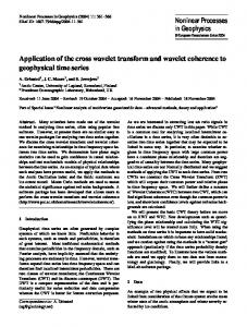
In 1998, Kingsbury first introduced the DT CWT [Kin98], that relies on the observation that approximate shift invariance can be achieved with a real DWT by doubling the sampling rate at each level of the tree. For this to work, the samples must be evenly spaced. The sampling rates can be doubled by eliminating the down-sampling by 2 after the level 1 filters. This is equivalent to having two parallel fully-decimated trees a and b, like in fig. 3.4, provided that the delays of H0b and H1b are one sample offset from H0a and H1a . Kingsbury found that, to get uniform intervals between samples from the two trees below level 1, the filters in one tree must provide delays that are half a sample different (at each filter input rate) from those in the other tree. This statement is also supported by Selesnick who, in [Sel01], gives an alternative derivation and explanation of the same result. The implementation of such a transform is done using two mother wavelets, one for each tree, one of them being (approximately) the Hilbert transform of the other. On one hand, the dual-tree DWT can be viewed as an overcomplete wavelet transform with a redundancy factor of two. On the other hand, the dual-tree DWT is also a complex DWT, where the first and second DWTs represent the real and imaginary parts of a single complex DWT. The first implementation proposed had the constraint of linear phase, and to accomplish this, the implementation required odd-length filters in one tree and even-length filters in the other. Greater symmetry between the two trees occurs if each tree uses odd and even filters alternately from level to level, but this is not essential. In another implementation proposed in [Kin01], the condition of linear phase is dropped, resulting the so-called Q-shift dual tree. In this case all the filters beyond level 1 are even length and are designed to have a group delay of approximately 41 sample (+q). The required delay difference of 21 sample (2q) is then achieved by using the time reverse of the tree a filters in tree b so that the delay then becomes 3q. Furthermore, because the filter coefficients are no longer symmetric, it is now possible to design the perfect-reconstruction filter sets to be orthonormal, resulting that all filters beyond level 1 are derived from the same orthonormal prototype set. The design of such Q-shift filters and of odd/even filters is quite complicated; it can be done only through approximations and is largely presented in [Kin01] and, respectively [Kin98]. In order to have a visual aspect of the DT CWT, we present in figure 3.4, the Q-shift version of the DT CWT as it is given in [Kin01]. Shift Invariance In order to examine the shift invariance properties of a transform, Kingsbury [Kin01] proposes a method based on the retention of just one type (details or approximations), from just one level of the decomposition tree. For example one might choose to retain only the level-3 detail coefficients and set all the others to zero. If the signal y reconstructed from just these coefficients, is free of aliasing then it can be said that the transform is shift invariant at that level. The degree of shift invariance of two implementation schemes (one for the DT CWT and the other for the classical DWT) is presented in fig. 3.5.


41

Figure 3.4: The Q-shift version of the DT CWT, giving real and imaginary parts of complex coefficients from tree a and tree b respectively.

In each case the input is a unit step, shifted to 16 adjacent sampling instants in turn. Each unit step is passed through the forward and inverse version of the chosen wavelet transform. The figure shows the input steps and the components of the inverse transform output signal, reconstructed from the wavelet coefficients at each of levels 1 to 4 in turn and from the scaling function coefficients at level 4. Summing these components reconstructs the input steps perfectly. Good shift invariance is shown when all the 16 output components from a given level have the same shape, independent of shift. It is easily observed that the DT CWT has outstanding performances in this direction compared to the severe shift dependence of the normal DWT. 3.4.1.2

Two-dimensional DT CWT

Extension of the DT CWT to two dimensions is achieved by separable filtering along columns and then rows. However, if column and row filters both suppress negative frequencies, then only the first quadrant of the 2-D signal spectrum is retained. It is well known, from 2-D Fourier transform theory, that two adjacent quadrants of the spectrum are required to represent fully a real 2-D signal. Therefore in the DT CWT it is also filtered with complex conjugates of the row (or column) filters in order to retain a second (or fourth) quadrant of the spectrum. This then gives 4:1 redundancy in the transformed 2-D signal. A schematic representation of the 2D DT CWT based on the even-odd implementation was given by Jalobeanu et. al. [JBFZ03]. At level m = 1, the 2D DT CWT is simply a non-decimated wavelet transform (using a pair of odd-length filters ho and g o ) whose coefficients are re-ordered into 4 interleaved images by using their parity. This defines the 4 trees T = A, B, C and D. If a and d denote approximation and detail coefficients


42

Figure 3.5: Detail and approximation components at levels 1 to 4 of 16 shifted step responses of the DT CWT (a) and real DWT (b) (a0 = x, the input image), we have: Tree T (a1T )x,y dT1,1 x,y dT1,2 x,y dT1,3 x,y

A (a ∗ ho ho )2x,2y (a0 ∗ g o ho )2x,2y (a0 ∗ ho g o )2x,2y (a0 ∗ g o g o )2x,2y 0

B (a ∗ h h )2x,2y+1 (a0 ∗ g o ho )2x,2y+1 (a0 ∗ ho g o )2x,2y+1 (a0 ∗ g o g o )2x,2y+1 0

o o

C (a ∗ h h )2x+1,2y (a0 ∗ g o ho )2x+1,2y (a0 ∗ ho g o )2x+1,2y (a0 ∗ g o g o )2x+1,2y 0

o o

D (a ∗ h h )2x+1,2y+1 (a0 ∗ g o ho )2x+1,2y+1 (a0 ∗ ho g o )2x+1,2y+1 (a0 ∗ g o g o )2x+1,2y+1 0

o o

For all other scales (m > 1), the transform involves an additional pair of filters, even-length, denoted he and g e . There must be a half-sample shift between the trees to achieve the approximate shift invariance. Therefore, different length filters are used for each tree, i.e. it is necessary to combine he , g e with ho , g o , the 4 possible combinations corresponding to the 4 trees: Tree T am+1 T x,y m+1,1 dT x,y dm+1,2 T x,y dm+1,3 T x,y

(am A (am A (am A (am A

A ∗ he he )2x,2y ∗ g e he )2x,2y ∗ he g e )2x,2y ∗ g e g e )2x,2y

(am B (am B (am B (am B

B ∗ h h )2x,2y+1 ∗ g e ho )2x,2y+1 ∗ he g o )2x,2y+1 ∗ g e g o )2x,2y+1 e o

(am C (am C (am C (am C

C ∗ h h )2x+1,2y ∗ g o he )2x+1,2y ∗ ho g e )2x+1,2y ∗ g o g e )2x+1,2y o e

(am D (am D (am D (am D

D ∗ h h )2x+1,2y+1 ∗ g o ho )2x+1,2y+1 ∗ ho g o )2x+1,2y+1 ∗ g o g o )2x+1,2y+1 o o


43

The trees are processed separately, as in a real transform. The combination of odd and even filters depends on each tree. The transform is achieved by a fast Filter Bank (FB) technique, of complexity O (N ). The reconstruction is done in each tree independently, by using the dual filters. To obtain a0 , the results of the 4 trees are averaged. This ensures the symmetry between them, thus enabling the desired shift invariance. The complex coefficients are obtained by combining the different trees together. If the subbands are indexed by k, the detail subbands dm,k of the parallel trees A, B, C and D are combined m,k m,k to form complex subbands z+ and z− , by the linear transform: m,k m,k m,k m,k + j d + d z+ = dm,k − d B C A D m,k m,k m,k m,k z− = dm,k + d + j d − d A D B C (3.8) Shift Invariance The main property of the 2D DT CWT is the quasi shift invariance, as shown by Kingsbury [Kin01] i.e. the magnitudes |z± | are nearly invariant to shifts of the input image. The shift invariance is perfect at level 1, and approximately achieved beyond this level: the transform algorithm is designed to optimize this property. In fig. 3.5, the shift-dependence properties of the DT CWT were compared with the DWT for one-dimensional step functions. A similar comparison in the 2-D is presented in fig. 3.7. The input is now an image of a light circular disc on a dark background (see fig. 3.6). This circular form is suited for the analysis of the shift dependence in 2D as neighbor pixels from the contour of the disc can be interpreted as obtained through 2D shifts. The upper row of images, from left to right in fig. 3.7, show the components of the output image, reconstructed from the DT CWT wavelet coefficients at levels 1, 2, 3 and 4 and from the scaling function coefficients at level 4. The lower row of images show the equivalent components when the fully decimated DWT is used instead. In the lower row, we see substantial aliasing artifacts, manifested as irregular edges and stripes that are almost normal to the edge of the disc in places. Contrast this with the upper row of DT CWT images, in which artifacts are virtually absent. The smooth and continuous images here demonstrate good shift invariance because all parts of the disc edge are treated equivalently; there is no shift dependence. Directional Selectivity Complex filters in multiple dimensions can provide true directional selectivity, despite being implemented separably, because they are still able to separate all parts of the m-D frequency space. For example a 2D DT CWT produces six bandpass subimages of complex coefficients at each level, which are strongly oriented at angles ±15◦ , ±45◦ , ±75◦ , as illustrated by the level 4 impulse responses in fig. 3.8(a). In order to obtain these directional responses, it is necessary to interpret the scaling function (lowpass) coefficients from the two trees as complex pairs (rather than as purely real coefficients at double rate) so that they can be correctly combined with wavelet (highpass) coefficients, which are also complex, to obtain the filters oriented at ±15◦ and ±75◦ (see 3.8). The


44

Figure 3.6: Input image used for the 2D shift sensitivity test

2D DT CWT is directionally selective because the complex filters can separate positive and negative frequency components (due to the analyticity of the transform) in 1D, and hence separate adjacent quadrants of the 2D spectrum. In figure 3.9 is presented an example of directionally selective subbands obtained at four decomposition levels of the 2D DT CWT applied on the image ‘Lena’. The positive orientations are grouped in the left part while the negative orientations are in the right part. The decomposition levels are represented in the 2D DWT’s traditional manner; at each decomposition level there are three detail subbands for positive orientations and other three detail subbands for negative orientations. The similarity between the subimages corresponding to the same type of details of a given orientation from successive decomposition levels can be observed. The increasing of the absolute value of the details with the decomposition level can be also noticed. The image Lena is not symmetrical, the orientation of 45◦ being better represented than the orientation −45◦ due to the contours of the hat. This asymmetry can be observed analyzing the corresponding subbands in figure 3.9. Rotational Invariance The directionality of the 2D DT CWT renders it nearly rotation invariant in addition to nearly shift invariant. Figure 3.7 illustrates the image obtained by reconstruction from only one level coefficients of the real DWT and of the DT CWT for a test image with a sharp edge on a hyperbolic trajectory. The ringing and aliasing artifacts in the DWT coefficients that change with the edge orientation are not present in the CWT coefficients. This may be due also to the fact that each image in 3.7 is using coefficients from all six directional subbands at the given wavelet level. The only rotational dependence is a slight thinning of the rings of the bandpass images near orientations of ±45◦ and ±135◦ , due to the diagonal subbands having higher center frequencies than the others.


45

Figure 3.7: Wavelet and scaling function components at levels 1 to 4 of an image using the 2D DT CWT (upper row) and 2D DWT (lower row). Only half of each wavelet image is shown in order to save space.

3.4.2

Projection-based CWTs

Another class of Complex Wavelet Transforms is represented by the set of projectionbased non-redundant complex wavelet transforms (NRCWT), introduced by Fernandes et. al., [FvSB03]. The projection (mapping) represents the conversion of a real signal to an analytic (complex) form through digital filtering. NRCWT is basically the DWT of the complexvalued projection. While this type of transforms are restricted to IIR filters, they produce orthogonal solutions. Fernandes’ projection-based CWT (PCWT) uses flexible design techniques to trade-off between redundancy and shift-invariance. The implementation of the mapping-based complex wavelet transform is presented in fig. 3.10. The forward CWT consists of an arbitrary DWT filter-bank preceded by a mapping stage. The CWT is then inverted by appending an inverse-mapping stage after an inverse-DWT filterbank. The independence of the two stages in the PCWT implementation (the complex mapping and the DWT) allows them to be performed separately and alternatively, leading toward a greater flexibility through the implementation. In true sense, all of the class of NRCWT, which are designed to mitigate all three disadvantages of standard DWT, are not exactly non-redundant CWT. For instance, Fernandes’ implementation has a redundancy factor of 2.67 in two dimensions. These complex wavelet transforms are considered NRCWTs because of their two main design constraints. The first condition that must be fulfilled by these transforms is to offer


46

(a) DT CWT

(b) DWT

Figure 3.8: Basis functions of 2D Q-shift complex wavelets (top) and 2D real wavelet filters (bottom), all illustrated at level 4 of the transforms. The complex wavelets provide 6 directionally selective filters, while real wavelets provide 3 filters, only two of which have a dominant direction

controllable redundancy, equal or less to the redundancy of the DT CWT, while preserving all the benefits introduced by the DT CWT. Second constraint is to offer improved directionality and phase information with perfect non-redundancy at the cost of increased shift-sensitivity. Unlike other redundant complex wavelet transforms, such as DT CWT, that also mitigate DWT shortcomings, the decoupled implementation of PCWT (from a class of NRCWT) (see fig. 3.10) has two important advantages. First, the controllable redundancy of the mapping stage offers a balance between the degree of shift sensitivity and the transform’s redundancy. The second advantage of PCWT is the flexibility to use any DWT in the transform implementation. Analyzing the DT CWT, Magarey and Kingsbury [KM97] showed that the complex coefficient obtained at the output of this transform can also be obtained using a single DWT tree based on a quasi-analytic wavelet. Fernandes et al. [FvSB03] pointed out that there is yet another interpretation for the DT CWT coefficients: they may be interpreted as the DWT of the analytic signal associated with the input signal. For an L2 (R) input, the analytic signal is defined in this case as the Hardy-space image of the input signal. The classical Hardy-space H 2 (R → C) is defined by: H 2 (R → C) ≡ f ∈ L2 (R → C) : F (ω) = 0 for a. e. ω < 0 . Let the superscript ‘H’ denote the isomorphic Hardy-space image (or Hardy-space map-


47

Figure 3.9: Components from each subband of the reconstructed output image for a 4-level 2D DT CWT decomposition of Lena (central part (128x128) only)

Figure 3.10: Projection-based CWT and its inverse

ping) of an L2 (R) function. Then, the Hardy-space image of a function f is given by F H (ω) = F (ω) χ[0,∞) (ω) , resulting that f H has half the bandwidth of f . The other important term related to this complex mapping is ‘unitary map’. The unitary map is a linear, bijective, inner-product preserving map. The function spaces that are related through unitary map are called isomorphic to each other. The unitary map or isomorphism is realizable if it can be implemented through digital filter. Thus, complex or Hardy space projection of a real signal is said to be realizable if it is possible to use some form of digital filtering for the mapping. If we consider f P to be the projection of an L2 (R) function onto the scaling space V1 so that f (x) = n c (n) φ (x − n) or, equivalently, F (ω) = C (ω) Φ (ω) then, the H Hardy-space image f is given by F H (ω) = χ[0,∞) (ω) C (ω) Φ (ω). Unfortunately, since χ[0,∞) (ω) is not 2π-periodic, it cannot be applied to the scaling-coefficient sequence c using a digital filter, meaning that the Hardy-space mapping of an L2 (R) signal is impossible to compute.


48

To circumvent this obstacle, Fernandes [FvSB03] defined a new function space called the Softy-space, S + . The Softy-space is an approximation to Hardy-space and, moreover, the Softy-space mapping of an L2 (R) signal may be computed using a digital mapping filter h+ with magnitude response shown in fig. 3.11.

Figure 3.11: |H + (ω)|, the magnitude response of the mapping filter h+ By suppressing the negative frequencies of an input signal, h+ maps the signal onto the Softy-space. The triangle in fig. 3.12 depicts the relationship between these function spaces.

Figure 3.12: Relationship between L2 (R), Hardy-space and Softy-space The PCWT is defined to be the DWT of the Softy-space image of an L2 (R) function, as shown in fig. 3.13. The mapping-filter h+ is used to project an L2 (R) function f onto the Softy-space. Since h+ is a complex-coefficient filter, it introduces a redundancy factor of two when applied to a real-valued scaling-coefficient sequence. It is then computed the DWT of the Softy-space mapping f + to obtain the CWT coefficients that will undergo application-specific processing. After the IDWT, an inverse-mapping filter g + computes the L2 (R) processed function f . Since f + ≈ f H , the CWT will have approximate shiftability. In order to eliminate the data redundancy, the non-redundant mapping scheme shown in fig. 3.14 is proposed. As depicted in the figure, the non-redundant mapping is defined as the concatenation of a mapping filter and a downsampler (elimination of odd-indexed scaling coefficients). The downsampler eliminates the redundancy created by the mapping filter that generates complex scaling coefficients from real scaling coefficients. It can be observed that the scaling-coefficient sequences c and e c+ can both be represented by N real numbers within a digital computer; therefore, there is no data redundancy in the scaling-coefficient sequence and e c+ .


49

Figure 3.13: PCWT

Figure 3.14: Non-redundant mapping

3.4.3

Hyperanalytic Wavelet Transform

In this section, a very simple implementation of the HWT is introduced. I will begin by presenting the 1D case, highlighting the shift-invariance properties and I will continue with the 2D case and insist both on the quasi shift-invariance and directional selectivity. 3.4.3.1

Analytical Discrete Wavelet Transform (ADWT)

As discussed in the previous chapter, a 1D wavelet transform (WT), is shift-sensitive if an input signal shift causes an unpredictable change of the transform coefficients. Shiftsensitivity is an undesirable property because it implies the impossibility to distinguish between wavelet transform coefficients corresponding to input signal shifts. The shiftsensitivity of the DWT is generated by the down-samplers used for its computation. Throughout time, there were numerous attempts to overcome this disadvantage. A straight-forward solution is to remove the downsamplers from the DWT’s implementation, resulting the UDWT [Mal99], [LGO+ 96]. Although the UDWT is shift-insensitive, it has high redundancy (equal to 2J , where J denotes the number of iterations), caused by the absence of down-samplers. Unfortunately, the high redundancy incurs a massive storage requirement that makes the UDWT inappropriate for most signal processing


50

applications. Another disadvantage of the UDWT comes from the fact that it requires the implementation of a large number of different filters. Lang, Guo, Odegard, Burrus and Welles [LGO+ 96] have proposed a new shift-invariant but very redundant wavelet transform, named Shift Invariant Discrete Wavelet Transform, SIDWT. Their proposition is based on a translation invariant algorithm proposed by Coifman and Donoho [CD95]. The computation of this transform implies the consideration of all circular shifts of the input signal. After the computation of the DWT of every shifted version of the signal, this method requires the shifting back (or unshifting) and averaging over all results obtained. The method introduced by Coifman and Donoho in [CD95] and called Cycle Spinning (CS) was conceived to suppress the artifacts in the neighborhood of discontinuities introduced by the classical DWT in denoising applications, and it implies the rejection of the translation dependence. For a range of shifts, data (time samples of a signal) is shifted (right or left as the case may be), the DWT of shifted data is computed, and than the result is un-shifted. Doing this for a range of shifts, and averaging the several results so obtained, a quasi shift-invariant discrete wavelet transform is obtained. The degree of redundancy of this transform is proportional to the number of shifts of the input signal produced. Cycle spinning over the range of all circular shifts of the input signal is equivalent to SIDWT. Abry [Abr94], first demonstrated that approximate shiftability is possible for the DWT with a small, fixed amount of transform redundancy. He designed a pair of real wavelets such that one is approximately the Hilbert transform of the other. This wavelet pair defines a CWT. For explaining that such a transform is complex, consider the pair of DWT trees associated with the wavelet pair already mentioned. A complex wavelet coefficient is obtained by interpreting the wavelet coefficient from one DWT tree as being its real part, whereas the corresponding coefficient from the other tree is interpreted as its imaginary part. This transform is represented in figure 3.15(a).

(a) Previous ADWT implementations

(b) Proposed ADWT implementation

Figure 3.15: Equivalent implementations of the ADWT In 3.15(b) we propose a new implementation of the complex wavelet transform, similar to the DTCWT but easier to implement, [AOB06]. It involves computing a single


51

DWT but, instead of applying it to the original signal we apply it to the analytical signal associated with our input signal. The analytic signal is defines as in 3.2. These implementations of the ADWT, presented in fig. 3.15 are equivalent because, taking into consideration the properties of the inner product and the ‘anti-self adjointness’ of the Hilbert transform, namely hH {u} , vi = hu, −H {v}i with u ∈ Lp (R) and v ∈ Lq (R), we can write the wavelet coefficients of the ADWT, at level m, dm ADW T as follows:

m dm x (t) , ψa,n (t) ADW T [n] = = hx (t) , ψnm (t) + jH {ψnm (t)}i = hx (t) , ψnm (t)i − j hx (t) , H {ψnm (t)}i = hx (t) , ψnm (t)i + j hH {x (t)} , ψnm (t)i = hx (t) + jH {x (t)} , ψnm (t)i = hxa (t) , ψnm (t)i (3.9) In fact neither the DTCWT, nor the proposed implementation of ADWT correspond to perfect analytic mother wavelets, because the exact digital implementation of a Hilbert transform pair of mother wavelets with good performance is not possible in the case of the first transform (due to the fractional delay between the two trees required) and because the digital Hilbert transformer is not a realizable system in the case of the second transform, in practice this transformation being done only through approximations. Our proposal requires a implementation of the Hilbert transformer acting in the domain of the Fast Fourier Transform, as in figure 3.16. In simulations we have used the processing

Figure 3.16: The implementation of the Hilbert transformer scheme in 3.17.

Figure 3.17: The use of the Hilbert transform in simulations The DTCWT requires special mother wavelets but can assure a higher degree of shift invariance whereas the implementation of the ADWT proposed in figure 3.15(b) can use any classical mother wavelets (e.g. those from the Daubechies family, Symmlet family and others). Both transforms have in the 1D case a redundancy of 2.


52

Shift Invariance In order to evaluate the shift-invariance performance of ADWT, two types of simulations are performed. First, we make a visual evaluation of the degree of shift invariance by taking the same test prof. Kingsbury has proposed in [Kin01]. We have used this test to make a comparison between ADWT, DT CWT, and the classical DWT. As can be seen, we obtain results comparable with those obtained by Kingsbury, even though we have used Daubechies, 10-taps filter. From fig. 3.18 it can be observed that the DWT is not

Figure 3.18: A visual comparison ment to illustrate the shiftability of ADWT, DT CWT and DWT shift-invariant; the lines of coefficients corresponding to different shift are not parallel, while the ADWT and DT CWT are quasi shift-invariant. The second series of tests involves the computation of a ‘degree of shift-invariance’ that I have introduced. In [SFAH92], Simoncelli has defined a new measure of the shiftinvariance, called ‘shiftability’. According to their definition, a transform is shiftable if and only if any subband energy of the transform is invariant under input-signal shifts. Although weaker than shift invariance, shiftability is important for applications because it is equivalent to interpolability, which is a property ensuring the preservation of transformsubband energy under input-signal shifts. Based on this observation, we introduced a new criterion: the degree of shift invariance. In order to calculate this measure, we compute the energies of every set of detail coefficients (at different decomposition levels) and of the approximation coefficients, corresponding to a certain delay (shift) of the input signal samples. This way, I obtain a sequence of energies at each decomposition level, each


53

sample of this sequence corresponding to a different shift. Then the mean m and the standard deviation d of every energy sequence are computed. My degree of invariance is defined as: Deg = 1 − d/m (3.10) I perform the normalization with respect to the mean of the energy sequence because I want the values of the degree of invariance to be within the interval [0, 1], in order to facilitate its interpretation. If the transform is shift-invariant, then the value of its degree of invariance is 1 because the standard deviation of the energy sequence is zero in this case. The reciprocity is not guaranteed. There are quasi shift invariant wavelet transforms with the degree of shiftinvariance equal to 1 that are not perfectly shift-invariant. However, generally, when the transform is not shift-invariant the value of this degree of invariance is smaller than 1. This observation is also sustained by experimental work. We consider that the degree of shift invariance is an objective way of analyzing the shift invariance of a transform. In simulations, I have used as input signal a unitary step, like in 3.18. In fact, 16 different unitary steps were used. They were generated one from another by delaying with a sample. The number of iterations used for the computation of the DWT was 3. I repeated the simulations for several mother wavelets commonly used in the literature (Daubechies, Symmlet and Coiflet). In order to isolate the coefficients corresponding to each level, after the computation of the corresponding forward WT, all the coefficients corresponding to the other levels are set to zero, by applying a ‘mask’ on the sequence obtained. For a better understanding of this procedure, I illustrate in figure 3.19 the system used for the analysis of the shift invariance at the 3rd decomposition level of the ADWT.

Figure 3.19: The system used for the shift-invariance analysis of the third level of the wavelet decomposition. In this example is considered the case of the proposed implementation of ADWT The inverse ADWT (IADWT) can be implemented using the systems proposed in [FIB09], [ANBI07b], [FIBI09] and [FNBI09]. In the first test involving the values of the degree of shift invariance I have compared its values obtained for our transform with the values obtained in the case of the CS with


54

a various number of cycle spins and for a variety of spinning steps (a spinning step is the number of samples the signal is shifted once). In table 3.1 I present a comparison between my transform and the CS. This comparison is based on the values of the degree of shift invariance calculated for the approximation coefficients obtained after the 3rd iteration of the corresponding WT computation algorithm (Scaling fn., level 3), for the detail coefficients obtained after the 3rd iteration (Wavelets level 3), for the detail coefficients obtained after the 2nd iteration (Wavelets level 2) and for the detail coefficients obtained after the 1st iteration (Wavelets level 1). It can be observed, analyzing this table, that the ADWT is equivalent to the CS with redundancy 64, from the degree of shift-invariance point of view. Symmlet, 10 Redundancy Scaling fn. level 3 Wavelets level 3 Wavelets level 2 Wavelets level 1 Daubechies, 10 Scaling fn. level 3 Wavelets level 3 Wavelets level 2 Wavelets level 1

ADWT 2 0,8594 0,9962 0,9963 0,9992 ADWT 0,8594 0,9981 0,9982 0,9992

CS step=1,64 delays 64 0,7551 0,9962 0,9965 0,9985 CS step=1, 64 delays 0,7551 0,9965 0,9968 0,9985

CS step=1, 512 delays 512 0,7551 0,9995 0,9996 0,9998 CS step=1, 512 delays 0,7551 0,9996 0,9996 0,9998

Table 3.1: A comparison between two quasi shift-invariant WTs, the ADWT and the CS Another test involved the dependency of the degree of shift invariance of the proposed WT with respect to the regularity of the mother wavelet used for its computation. I investigated the Daubechies family, each element being indexed by its number of vanishing moments. As the curve illustrated in figure 3.20 indicates, the degree of shift-invariance increases with the regularity of the mother wavelets used.

Figure 3.20: The dependency of the degree of shift-invariance of HWT on the regularity of the mother wavelet used for its computation Finally, in table 3.2 I have put the values of this degree computed for the signals deployed in fig. 3.18. As it can be seen, my new implementation is comparable with the DT CWT both from the visual point of view and by analyzing the values of the degree of invariance.

3.4. Examples of Complex Wavelet Transforms WT ADWT DT CWT DWT

W. lev. 1 0.9967 1.0000 0.9236

Degree of invariance W. lev. 2 W. lev. 3 W. lev. 4 0.9995 0.9986 0.9988 0.9811 0.9749 0.9734 0.8265 0.7878 0.8149

55 Sn. lev. 4 0.9990 0.9997 0.9958

Table 3.2: A comparison of ADWT, DT CWT and DWT

3.4.3.2

Hyperanalytic Wavelet Transform (HWT)

All the 1D WTs already mentioned have simpler or more complicated 2D generalizations. The generalization of the analyticity concept in 2D is not obvious, because there are multiple definitions of the Hilbert transform in this case. In the following I will use the definition of the analytic signal associated to a 2D real signal named hypercomplex signal. So, the hypercomplex mother wavelet associated to the real mother wavelet, ψ (x, y) is defined as: ψa (x, y) = ψ (x, y) + iHx {ψ (x, y)} + jHy {ψ (x, y)} + kHx {Hy {ψ (x, y)}}

(3.11)

where i2 = j 2 = −k 2 = −1, ij = ji = k, jk = kj = −i, ki = ik = −j and ijk = 1, [Dav]. The HWT of an image f (x, y) is: HW T {f (x, y)} = hf (x, y) , ψa (x, y)i .

(3.12)

Replacing 3.11 in 3.12, we will obtain: HW T {f (x, y)} = hf (x, y) , ψ (x, y)i + hf (x, y) , iHx {ψ (x, y)}i + + hf (x, y) , jHy {ψ (x, y)}i + hf (x, y) , kHx {Hy {ψ (x, y)}}i = = hf (x, y) , ψ (x, y)i − i hf (x, y) , Hx {ψ (x, y)}i − −j hf (x, y) , Hy {ψ (x, y)}i + k hf (x, y) , Hx {Hy {ψ (x, y)}}i = = hf (x, y) , ψ (x, y)i − i h−Hx {f (x, y)} , ψ (x, y)i − −j h−Hy {f (x, y)} , ψ (x, y)i + k h−Hx {f (x, y)} , Hy {ψ (x, y)}i = = hf (x, y) , ψ (x, y)i + i hHx {f (x, y)} , ψ (x, y)i + +j hHy {f (x, y)} , ψ (x, y)i − k h−Hy {Hx {f (x, y)}} , ψ (x, y)i = = DW T {f (x, y)} + iDW T {Hx {f (x, y)}} + +jDW T {Hy {f (x, y)}} + kDW T {Hy {Hx {f (x, y)}}} = = hfa (x, y) , ψ (x, y)i = DW T {fa (x, y)} . (3.13) Based on 3.13 we can conclude that the HWT of the image f (x, y) can be computed with the aid of the 2D DWT of its associated hyper complex image. In consequence the HWT implementation uses four trees, each one implementing a 2D DWT, thus having a redundancy of four. The first tree is applied to the input image. The second and the third trees are applied to 1D Hilbert transforms computed across the lines (Hx ) or columns (Hy ) of the input image. The fourth tree is applied to the result obtained


56

Figure 3.21: HWT implementation scheme

after the computation of the two 1D Hilbert transforms of the input image. The HWT implementation is presented in figure 3.21, [ANBI07a]. In what concerns the reconstruction part, a possible method would be to reverse the Hilbert transform applied at the input (both Hilbert transforms in the last case) for each of the three trees mentioned above, and the final result to be the mean of the four images computed on the four trees. Shift Invariance To illustrate the quasi shift-invariance properties of the HWT, I have, once again, retaken one of Kingsbury’s tests, presented in fig. 3.7, the results obtained being depicted in fig. 3.22. In this case the wavelet used in the computation of the HWT has been Daubechies with 10 vanishing moments. Analyzing the results in 3.22 we can conclude that the two complex WTs outperform the 2D DWT, the behavior of the HWT being quite similar to the behavior of the 2D DTCWT. Directional Selectivity The enhancement of the directional selectivity of the HWT is made, as in the case of the 2D-DTCWT, [Kin98], [SBK05], through linear combinations of detail coefficients belonging to each subband of each of the four 2D-DWTs (see the right side of fig. 3.21). Let us consider, for example, the case of the diagonal detail subbands, (HH), presented in figure 3.23. I have selected a particular input image, f (x, y)) = δ (x, y), to appreciate the frequency responses associated to different transfer functions represented in figure 3.21 [ANBI07b]. More precisely, the example in figure 3.23 refers to the transfer functions that relate the input f with the outputs z−r and z+r . The spectrum of the input image, F {δ (x, y)} (fx , fy ) is constant. The wavelet coefficients belonging to the subband HH are obtained by lines and columns high-pass filtering.


57

Figure 3.22: Comparison in the 2D case between the HWT, the DT CWT and the DWT

I have assumed ideal high-pass filters. The spectra of the wavelet coefficients d1 , d2 , d3 , d4 belonging to the subband HH, denoted by F {DW THH {δ (x, y)}}, F {DW THH {Hx {δ (x, y)}}} , F {DW THH {Hy {δ (x, y)}}} and, respectively, F {DW THH {Hy {Hx {δ (x, y)}}}}, have two preferential orientations, corresponding to the two diagonals ±π/4. These directions are the result of the fact that 2D DWT cannot separate these two orientations. After the linear combinations proposed, we can observe of the that the spectra coefficients so obtained, for example z−r and z−r , F HHz−r (fx , fy ) and F HHz+r (fx , fy ), have only one preferential direction, namely the second diagonal, respectively the first one. In conclusion, by using the HWT these directions can be separated. The same strategy can be used to enhance the directional selectivity in the other two subbands: LH and HL, obtaining the preferential orientations at ±atan (2) and ±atan (1/2). A comparison of the directional selectivity of the 2D DWT and HWT, implemented as proposed in figure 3.21, is presented in figure 3.24. I have conceived a special input image, in the frequency domain, to conduct this simulation. Its spectrum, represented in figure 3.24, is oriented following the directions: 0, ±atan (1/2), ±π/4, ±atan (2) and π.

3.5. Advantages and Applications of Complex Wavelet Transforms

58

Figure 3.23: The strategy of directional selectivity enhancement in the HH subband illustrated through the transfer functions of the systems used in the HWT implementation

Like the 2D DTCWT, the HWT implemented as proposed in figure 3.21, has six preferential orientations: ±atan (1/2), ±π/4 and ±atan (2). The 2D-DWT has only three preferential orientations: 0, π/4 and π/2, it does not make the difference between the two principal diagonals. The better directional selectivity of the proposed implementation of HWT versus the 2D DWT can be easily observed, comparing the corresponding detail sub-images in figure 3.24. For the diagonal detail sub-images, for example, the imaginary part of the HWT rejects the directions: −atan (1/2), −π/4 and −atan (2), whereas the 2D DWT conserves these directions.

3.5

Advantages and Applications of Complex Wavelet Transforms

The advantages of the complex wavelet transforms lay in the reason they were introduced in the first place, namely decreased shift sensitivity and increased directional selectivity.

3.5. Advantages and Applications of Complex Wavelet Transforms

59

Figure 3.24: The absolute values of the spectra of horizontal and diagonal detail subimages obtained after the first iterations of 2D DWT and HWT. In the HWT case, the real and imaginary parts of complex coefficients are separated

Although these goals might be achieved with real wavelet transforms (UDWT is shift invariant and DWPT offers good directional selectivity), complex wavelets transforms manage to obtain good results in these directions while preserving a reasonable amount of redundancy. When talking about the specific complex wavelet transforms presented above, each of them has advantages and limitations, the latter resulting mainly from the fact that there is impossible to compute an analytic signal using digital filters. In what concerns the applications of the complex wavelet transforms, they cover mainly the area of signal and image processing were the advantages introduced with the price of increased redundancy are significant. A description of these advantages is nicely presented in [Kin01], [Shu03] and [SBK05]. One of the most important applications in signal and image processing is denoising. In what concerns signals, apparently many denoising methods perform better when associated with shift-invariant wavelet transforms. In the case of images, the increased di-

3.6. Summary

60

rectional selectivity in addition to shift-invariance leads to better performances especially when it comes to images containing significant diagonal edges. Directional selectivity is a desirable feature when dealing with textures, in applications like texture analysis and synthesis and also in image segmentation and classification. Other possible applications include motion estimation and compensation, watermarking, deconvolution, coding, traffic applications [SI10] and so on.

3.6

Summary

In this chapter I have introduced the complex wavelet transform, focusing on the theoretical approach (the analytic wavelet transform - not realizable in practice), continued with the presentation of two classes of CWTs, namely the dual-tree based complex wavelet transforms and the projection-based complex wavelet transforms. For each of these classes I have taken a representative complex wavelet transform and presented it in large. Finally I have presented my own contribution to this domain, namely the implementation of the Hyperanalytic Wavelet Transform, which permits the exploitation of the mathematical results and of the algorithms previously obtained in the evolution of wavelets theory. This implementation has a very flexible structure, as we can use any orthogonal or bi-orthogonal real mother wavelets for the computation of the HWT. I have also illustrated its performances with the results of a few simulation tests. In the following chapter I will focus on the denoising of images based on the theory of wavelets and I will present some simulations based on the use of the HWT.

Chapter 4 Denoising 4.1

Introduction

In common use, the word ‘noise’ refers to any unwanted sound. In both analog and digital electronics, noise is an unwanted perturbation to a wanted signal; it is called noise as a generalization of the audible noise heard when listening to a weak radio transmission. Signal noise is heard as acoustic noise if played through a loudspeaker and it manifests as ’snow’ on a television or video image. Noise can block, distort, change or interfere with the meaning of a message in both human and electronic communication. In signal processing or computing it can be considered unwanted data without meaning; that is, data that is not being used to transmit a signal, but is simply produced as an unwanted by-product of other activities. The term ‘denoising’, also known as ‘noise reduction’ refers to the removal of noise.

4.1.1

Digital images and noise

Images taken with both digital cameras and conventional film cameras will record noise from a variety of sources. Many further uses of these images require that the noise will be (partially) removed - for aesthetic purposes as in artistic work or marketing, or for practical purposes such as computer vision. Depending on the model used to characterize the noise, we can encounter ‘salt and pepper’ noise, gaussian noise and many others. Another possible classification takes into consideration the way the noise affects the image, resulting in additive noise and multiplicative noise. The case of additive noise will be presented in this chapter, while the multiplicative noise will be discussed in chapter 5. In Gaussian noise, each pixel in the image will be changed from its original value by a (usually) small amount. A histogram, a plot of the amount of distortion of a pixel value against the frequency with which it occurs, shows an estimation of the distribution of noise. While other distributions are possible, the Gaussian (normal) distribution is usually a good model, due to the central limit theorem that says that the sum of independent noises tends to approach a Gaussian distribution. The case of Additive White Gaussian Noise (AWGN) will be considered. The acquired

61

4.1. Introduction

62

image is expressed in this case in the following form: x=s+n

(4.1)

where x is the observed/acquired image, s is the noiseless input image and n is the AWGN component. In salt and pepper noise (sparse light and dark disturbances), pixels in the image are very different in color or intensity from their surrounding pixels; the defining characteristic is that the value of a noisy pixel bears no relation to the color of surrounding pixels. Generally this type of noise will only affect a small number of image pixels. When viewed, the image contains dark and white dots, hence the term salt and pepper noise. Typical sources include flecks of dust inside the camera, or with digital cameras, faulty CCD elements. The speckle noise is modeled as multiplicative noise, the observed image having the expression: x=s·n (4.2) where n represents the speckle. In either case, the noises at different pixels can be either correlated or uncorrelated; in many cases, noise values at different pixels are modeled as being independent and identically distributed, and hence uncorrelated.

4.1.2

Denoising algorithms

In his book, [Mal99], Mallat stated that the estimation of signals in additive noise is optimized by finding a representation that discriminates the signal from the noise. An estimation is calculated by an operator that attenuates the noise while preserving the signal. There is a big diversity of estimators used as denoising systems. A review of such systems can be found in [Bua07]. One may classify these systems in two categories: those directly applied to the signal and those who use a wavelet transform before processing. From the first category, we must mention the denoising systems proposed in [FKE07] and [WD00]. The first one is based on the shape-adaptive discrete cosine transform (SADCT), transform that can be computed on a support of arbitrary shape. The second one is a maximum a posteriori (MAP) filter that acts in the spatial domain. Linear operators have long predominated because of their simplicity, despite their limited performance. It is possible to keep the simplicity while improving the performance with non-linearities in a sparse representation. Optimizing an estimator requires taking advantage of prior information. Bayes theory uses a probabilistic signal model to derive estimators that minimize the average risk. These models are often not available for complex signals such as natural images. An alternative is offered by the minimax approach, which only requires knowing a prior set where the signal is guaranteed to be. The quasi minimax optimality of wavelet thresholding estimators is proved for piecewise regular signals and images.

4.1. Introduction

63

Performance evaluation criteria The Mean Square Error (MSE) and the Peak Signal to Noise Ratio (PSNR) are the two error metrics used to compare image processing (denoising, compression) quality. The MSE represents the cumulative squared error between the denoised and the original image, whereas PSNR represents a measure of the peak error. The lower the value of MSE, the higher the PSNR. To compute the PSNR, it is first calculated the mean-squared error using the following equation: PM,N 2 m=1,n=1 [Io (m, n) − Ii (m, n)] M SE = (4.3) M ·N In the previous equation, Ii is the input, noise-free image, Io is the output image (might be noisy or already denoised) and M and N are the number of rows and columns in the input image, respectively. Then PSNR is being computed using the following equation: R2 (4.4) P SN R = 10log10 M SE In the previous equation, R is the maximum fluctuation in the input image data type. For example, if the input image has a double-precision floating-point data type, then R is 1. If it has an 8-bit unsigned integer data type, R is 255, etc.

4.1.3

Local averaging and PDEs

Many classical image denoising methods are based on a local average. The restored value at a pixel is obtained as an average of its neighboring pixels. The most classical algorithm is the Gaussian filtering. In that case, the restored value is obtained as a weighted average where the weight at each pixel depends on the distance to the restored one. This low pass filter tends to blur the image. This is known as the ‘local average treatment effect’. The neighborhood filters avoid the blurring effect by restricting the average to pixels having a similar gray level value. The idea is that gray level values inside a homogeneous region slightly fluctuate while pixels belonging to different regions have a larger gray level difference. The neighborhood filter takes an average of the values of pixels which are simultaneously close in gray level value and spatial distance. One can involve calculus to interpret more in depth the neighborhood filters and improve them. In fact, expert photographers object to the creation of irregularities, in particular the flat tints and false details. In general, image filters can be better understood by establishing their asymptotic action when they are made more and more local. This action is then described by a Partial Differential Equation (PDE). A further inquiry has led us to discover that a very simple version of the neighborhood filter has a well posed subjacent PDE, namely the mean curvature motion. This variant simply consists of replacing the average by a linear regression in the formula defining the neighborhood filter. The improvement has been accepted by professionals.

4.1. Introduction

4.1.4

64

The total variation minimization

Total variation (TV) based filtering was introduced by Rudin et al. [ROF92]. TV denoising is an effective, robust filtering method for recovering piecewise-constant signals. Many algorithms have been proposed to implement total variation filtering. The total-variation of a signal measures how much the signal changes between signal values. Specifically, the total-variation of an N -point signal x (n), 1 ≤ n ≤ N is defined as: N X T V (x) = |x (n) − x (n − 1)| . (4.5) n=2

The total variation of x can also be written as: T V (x) = kDxk1 where

  D= 

−1

(4.6) 

1 −1 1

 , 

...

(4.7)

−1 1 is a matrix of size (N − 1) × N . We assume we observe the signal x corrupted by additive white Gaussian noise, y = x + n, y, x, n ∈ RN One approach to estimate x is to find the signal x that minimizes the objective function J (x) = ky − xk22 + λ kDxk1 . This approach is called TV denoising. The regularization parameter, λ, controls how much smoothing is performed. Larger noise levels call for larger λ. Many algorithms have been proposed to implement total variation filtering, and it still represents an active topic of research.

4.1.5

Properties of natural images

In this section are presented axioms and properties of images justified by the processing of observed natural images. Structural properties are defined, enabling the description of image contents with general statistical rules. These properties have precise consequences on image modeling. 1. Axiom A1: self-similarity. Natural phenomena are often self-similar, from a statistical point of view. As a result, natural images display scale invariance. This means that changing the scale of a signal (by studying only a small part of it for instance) does not change the statistical properties of the signal. When studying a statistic (e.g. the expectation of the power spectrum), the spatial shape of this statistic is not affected by scaling. The self-similarity can be associated with the notion of fractal, widely used to model objects such as mountains or coast lines.

4.1. Introduction

65

2. Axiom A2: spatial adaptivity. Natural images generally exhibit a strong spatial adaptivity, since they are composed of different textures, homogeneous areas, sharp edges and small features. The importance of having a spatially variant model is shown by the failure of stationary approaches to correctly model images, especially when dealing with inverse problems such as denoising or deblurring. However, taking into account the space-varying characteristics of a natural scene is a difficult task, since it requires the definition (followed by the estimation) of a large number of additional parameters, at least one per pixel. This can inevitably lead to over fitting issues, since the non stationary parameters can adapt more to the noise than to the underlying signal, if they are not subject to any constraint. The use of a prior probability density function helps to constrain these parameters and take advantage of the spatial adaptivity. 3. Property P1: inter-scale persistence. When dealing with scale invariant data, it is natural to use a multiresolution decomposition (e.g. wavelets) to analyze them. This enables us to get a sparser representation, and to separate the scale invariance from other properties. The underlying spatial structure of the image persists through the different scales, i.e. high/low value of the coefficient magnitudes often lead to high/low values at the next scale. This can be seen as the inability of any multiscale transform to perfectly decorrelate natural images, since such a transform exhibits some inter-scale redundancy. 4. Property P2: intra-scale dependencies. Now we consider two different subbands of the same scale, but with different orientations (they are generated by linear filtering with the same filter with respect to size and shape, but oriented differently). Homogeneous areas and details are found approximately at the same spatial location in the different subbands. Isotropic details, such as smooth areas and round features, are naturally found at all orientations. This shows again that multiscale transforms do not perfectly decorrelate the information contained in natural images. The best basis to represent such a process is the Karhunen-Loeve (K-L) basis. The image coefficients in this basis are independent. It is optimal, since it provides the minimum mean error when approximating an image by its projection on orthogonal basis vectors chosen a priori (this relates to image denoising by thresholding). For stationary processes, the K-L basis is the Fourier basis. However, the Fourier basis is not well suited to the nonstationarity of natural images. In the case of natural images a wavelet basis is the closest approximation to a K-L basis, since it provides both a frequency and a spatial representation. The fact that it is only an approximation is illustrated by the properties P1 and P2 (residual dependencies). The aim is not only to diagonalize a Gaussian process, but also to provide the shortest description of the useful signal. Modeling can be seen as finding a simple description of nature, and in this case it can be related to image compression. It is well-known that wavelets provide a compact representation of natural images, and are widely used in coding.

4.1. Introduction

66

An interesting consequence of the self-similarity is that high order statistics are scale invariant. It means that they obey a function f of the scale, and the shape of f is not affected by scaling (it is only multiplied by a scale factor). A generalization of this law is the scale invariance of the wavelet subband histograms, they relate to the full coefficient distribution instead of its order n moments.

4.1.6

Frequency domain filters

The effect of averaging the spatially closest pixels can also be achieved in the Fourier domain. The convolution of an image by a kernel k is equivalent to the multiplication of its Fourier transform by K. The average of the spatially closest pixels is then equivalent to the cancellation of the high frequencies. As the analogous spatial filter, this cancellation leads to the blurring of the image and a Gibbs effect. The optimal filter in the Fourier domain is the Wiener filter which does not cancel the high frequencies but attenuates them all. The coefficients with a magnitude over the noise standard deviation are nearly untouched while the coefficients with a lower value are reduced. By the use of the Fourier basis, global image characteristics may prevail over local ones. The presence of any boundary makes all the Fourier coefficients to have a meaningful value and therefore they are less attenuated. In that case, the flat zones which should be easily restored preserve a regular amount of noise. In order to avoid these effects, the basis must take into account more local features, as the wavelet transform and the local discrete cosine transform (DCT) do. David Donoho actually introduced the word denoising in association with the wavelet theory [DJ94]. Thresholding estimators are studied in wavelet and wavelet packet bases, where they are used to suppress additive noises and restore signals degraded by low-pass filters. Non-linear estimations from sparse representations are also studied for operators, with an application to power spectrum estimation. The multi-resolution analysis performed by the WT has been shown to be a powerful tool in order to achieve good denoising. In the wavelet domain, the noise is uniformly spread throughout the coefficients, while most of the image information is concentrated in the few largest ones (sparsity of the wavelet representation) [FBB01, SS02, PP06, AK05, GD06, LBU07, Shu05, ZS07, Olh07]. The most straightforward way of distinguishing information from noise in the wavelet domain consists of thresholding the wavelet coefficients. Soft-thresholding filter (stf) is the most popular strategy and has been theoretically justified by Donoho and Johnstone [DJ94]. They propose a three steps denoising algorithm: 1. the computation of the forward WT, 2. the filtering of the wavelet coefficients, 3. the computation of the IWT of the result obtained. They use the Discrete Wavelet Transform (DWT) and the stf. Because it is not made any explicit hypothesis on the noise-free image it results in a non-parametric method. Their unique statistical hypothesis refers to the noise, considered additive white and Gaussian (AWGN). The stf is used to put to zero all the wavelet coefficients with the

4.1. Introduction

67

absolute value smaller than a threshold. This threshold is selected to minimize the minmax approximation error. Consequently, regarding the three steps denoising algorithm, there are two tools to be chosen: the WT and the filter. In what concerns the first choice, in this chapter will be used the new implementation of the HWT. In [FBB01, PP06] was used the UDWT, in [SS02, AK05, Shu05] the DTCWT, and in [GD06, LBU07] the DWT. Concerning the second choice, numerous non-linear filter types can be used in the WT domain. A possible classification is based on the nature of the noise-free component of the image to be processed. Basically, there are two categories of filters: those built assuming only the knowledge of noise statistics (a non-parametric approach), and those based on the knowledge of both signal and noise statistics (a parametric approach). From the first category can be mentioned: the hard-thresholding filter, [DJ94], the stf [DJ94, Mal99], that minimizes the Min-Max estimation error and the Efficient SURE-Based Inter-scales Point-wise Thresholding Filter [LBU07], that minimizes the Mean Square Error (MSE). To the second category belong filters obtained by minimizing a Bayesian risk under a cost function, typically a delta cost function (MAP estimation [FBB01, SS02, AK05]) or the minimum mean squared error (MMSE estimation [PP06]). The denoising algorithms proposed in [SS02, PP06, AK05, GD06, LBU07] exploit the inter-scale dependence of wavelet coefficients. The method proposed in [PP06] takes into account the intra-scale dependence of wavelet coefficients as well. The statistical distribution of the wavelet coefficients changes from scale to scale. The coefficients of the WT have a heavy tailed distribution. To deal with this mobility, there are two solutions. The first one assumes the use of a fixed simple model, risking a decrease of accuracy across the scales. This way, there is a chance to obtain a closed form input-output relation for the MAP filter. Such an input-output relationship has two advantages: it simplifies the implementation of the filter and it allows the sensitivity analysis. The second solution assumes the use of a generalized model, defining a family of distributions and the identification of the best fitting element of this family to the distribution of the wavelet coefficients at a given scale (e.g. the family of Pearson’s distributions in [FBB01], the family of SαS distributions in [AK05] and the model of Gauss-Markov random field in [GD06]). The use of a generalized model makes the treatment more accurate but requires implicit solutions for the MAP filter equation, which can often be solved only numerically.

4.1.7

Non local averaging

Non-local (NL) means algorithms are proposed in [Bua07]. The NL-means algorithm tries to take advantage of the high degree of redundancy of any natural image. Every small window in a natural image has many similar windows in the same image. In a very general sense, one can define as ‘neighborhood of a pixel i’ any set of pixels j in the image so that a window around j looks like a window around i. All pixels in that neighborhood can be used for predicting the value at i. Given a discrete noisy image x = {x (i) |i ∈ I}, the estimated value, N Lx (i) is computed as a weighted average of all the pixels in the image, X N Lx (i) = β (i, j) x (j) , j∈I

4.2. Non-parametric Denoising

68

where the weights {β (i, j)}j depend on the similarity between the pixels i and j and P satisfy the usual conditions 0 ≤ β (i, j) ≤ 1 and j β (i, j) = 1. In order to compute the similarity between the image pixels, a neighborhood system on I is defined. While producing state-of-the-art denoising results, this method is computationally impractical [MS05]. Its high computational complexity is due to the cost of weights calculation for all pixels in the image during the process of denoising. For every pixel being processed, the whole image is searched, and differences between corresponding neighborhoods are computed. The complexity is then quadratic in the number of image pixels. In [MS05] the computational complexity of the algorithm proposed in [Bua07] is addressed in a different fashion. The basic idea proposed in [MS05] is to pre-classify the image blocks according to fundamental characteristics, such as their average gray values and gradient orientation. This is performed in a first path in [MS05], and while, denoising in the second path, only blocks with similar characteristics are used to compute the weights. Accessing these blocks can be efficiently implemented with simple lookup tables. The basic idea is then to combine ideas from [Bua07], namely, weighted average based on neighborhoods similarity, with concepts that are classical in information theory and were introduced in image denoising context. Images with much finer texture and details will not benefit that much from the denoising; while reducing most of the noise, this type of processing will inevitably degrade important image features [GSZ06]. The first problem is to distinguish between good and bad candidates for denoising. Many natural images exhibit a mosaic of piecewise smooth and texture patches. This type of image structure calls for position (spatial)-varying filtering operation. Textured regions are characterized by high local variance. In order to preserve the detailed structure of such regions, the level of filtering should be reduced over these regions. The basic concept amounts to a reduction in the extent of filtering in regions where signal power exceeds that of the noise. So, the solution proposed in [GSZ06] supposes the anisotropic treatment of the acquired image taking into account the local variance values of its regions. This procedure can be seen like an NL-means algorithm where the classification of the image blocks is done on the basis of their local variance.

4.2

Non-parametric Denoising

The term ‘non-parametric’ is used to define all the methods developed without an a priori knowledge of the distribution of the signal to be processed. This non-parametric approach is motivated by the fact that in most practical situations, the distribution of the signals forming the observation are not known and is difficult to estimate them precisely.

4.2.1

Basic Concept

Even though we do not have any information on the distribution of the signal to be estimated, it is possible to satisfactory estimate this signal if we have a basis that permits the noise discrimination. The idea is to consider the noise additive, white and Gaussian. It is known that the projection of this type of noise on an orthonormal basis does not change


69

the nature of the noise. Let there be an observation made up of a signal perturbed by additive white Gaussian noise. If we dispose of an orthonormal basis able to ‘concentrate’ this signal’s energy over a small number of high-amplitude coefficients, than the projection of the observation on such a basis will be made of a small class of relatively large coefficients (containing mainly the information on the signal) and a large class of small coefficients which are mainly due to the noise. The estimation implies recovering and, eventually, processing the large coefficients, after setting to zero the small ones. Such an estimation is realized with a so called ‘thresholding function’, named after the threshold underneath which every coefficients will be forced to zero. It is said that a basis able to concentrate a big part of the signal’s energy on a small number of coefficients does a sparse representation of the signal [DJ94]. This definition is not really precise as the terms ‘small’ and ‘big’ are not clearly defined, resulting in a sparse representation in a wide sense. It can be said about a basis that it realizes a sparse representation in a strict sense if, for a given signal, the energy of this signal is ‘almost entirely’ contained in a small number of high-amplitude coefficients. In this type of sparsity, almost all the coefficients qualified as ‘small’ are, in fact, almost nulls or with very low amplitudes, consequently not containing any significant information on the signal. In the case of the sparse representation in a wide sense, and not strictly sparse, it might be useful to process in equal manner the small coefficients. In this case it is being considered not a thresholding function but a so called attenuation function, in the sense that it does not force to zero all the small coefficients but it imposes them a higher attenuation than on the large coefficients.

4.2.2

Shrinkage Strategies

In order to realize the non-parametric estimation described before, one must choose a sparse representation and an appropriate attenuation function. When the attenuation function sets to zero all the coefficients inferiors to a threshold, than the function is called thresholding. Some of the most used thresholding function are the Hard Thresholding and the Soft Thresholding, Soft Thresholding The three-step denoising algorithm proposed by Donoho and Johnstone [DJ94], already mentioned, uses the DWT and the stf. They do not make any explicit hypothesis on the noise-free image and, consequently, this method can be considered non-parametric. Their unique statistical hypothesis refers to the noise, considered AWGN. The stf is used to put to zero all the wavelet coefficients with the absolute value smaller than a threshold. This threshold is selected to minimize the min-max approximation error. The input-output relation of the stf is given by:   Wx − t, for Wx > t ˆ 0, for |Wx | ≤ t Ws (Wx ) = (4.8)  Wx + t, for Wx < −t. where Wx = Ws + Wn and t represents a threshold. Wx represents the sequence of WT coefficients of the noisy image, Ws represents the sequence of the WT coefficients of


70

the noiseless component of the acquired image and Wn represents the sequence of WT coefficients of the noise in the acquired image. The interval (−t, t) is named dead zone, because all the detail WT coefficients having the values in this interval are set to zero by the stf. Because the magnitudes of all the detail WT coefficients are reduced by the stf, it is named shrinkage operator. If the threshold t is chosen accordingly with the value of the noise’s standard deviation, then this filter is called adaptive. The noise’s variance can be estimated using the relation: 2 = σ ˆW n

median (|Wx |) Wx ∈ D13 0.6745

(4.9)

PSNRo

In the case of the minimization of the Min-Max approximation error, the constant that multiplies the noise’s standard deviation in order to obtain the threshold value t is √ equal to 2lnN , where N represents the number of pixels of the observed image. Another value, specific for the criteria that demands the minimization of the output noise power, is 3 (having in mind the three sigmas rule, specific for the Gaussian laws). In the following we present an experiment that associates the Diversity Enriched Discrete Wavelet Transform (DE DWT - a transform whose result is the mean of 9 different DWTs, each one corresponding to a different mother wavelet from the Daubechies family) [IIA06] and the soft-thresholding filter. The optimization criteria (in this case the maximization of the output peak signal-to-noise ratio) demands the use of another value for the proportionality constant, between the threshold of the stf filter and the noise’s standard deviation. In the following simulations the value of this constant is chosen such that the PSNR associated to each DWT is maximum. The results obtained for the image Lena are presented in the folowing table. The values in this table were obtained by selecting each time a number of 6 iterations for the DWTs. σn PSNRi Daub,4 Daub,6 Daub,8 Daub,10 Daub,12 Daub,14 Daub,16 Daub,18 Daub,20 DE DWT

10 28.17 30.71 30.96 30.99 30.96 30.77 30.70 30.68 30.64 30.72 31.80

15 24.62 28.64 28.77 28.82 28.90 28.79 28.65 28.71 28.66 28.64 29.77

20 22.15 26.99 27.10 27.17 27.22 27.17 27.12 27.06 27.08 27.07 28.14

25 20.17 25.77 25.87 25.89 25.91 25.91 25.86 25.83 25.78 25.76 26.87

30 18.63 24.80 24.88 24.98 25.03 25.02 24.94 24.92 24.91 24.84 25.94

35 17.30 23.97 24.11 24.23 24.24 24.21 24.16 24.16 24.09 24.07 25.18

Table 4.1: PSNRs obtained using the soft-thresholding filter in the 2D DWTs domain, computed using the mother wavelets from the Daubechies family and in the DE DWT domain, for the image Lena perturbed with AWGN with different variances


71

Hard Thresholding Another type of non-parametric filter is the hard-thresholding filter (Htf). This is also a shrinkage operator. The input-output relation of this filter is: y, for |y| ≥ t hard (y, t) = (|y| − t)+ = (4.10) 0, for |y| < t where

(X)+ =

X, for X > 0, 0, otherwise.

(4.11)

PSNRo

This filter also has a dead zone. Next, the results of some simulations on the association of the DWT and ED DWT with a hard thresholding filter are presented. The optimization criterion (in this chapter it is the PSNR maximization) demands for another value of the proportionality constant, between the threshold value and the standard deviation of the noise. In the following simulations the value of this constant is chosen to insure that the PSNR value associated to each DWT is maximum. The results obtained are presented in the following table. The values in the table correspond to a number of six iterations for each DWT. σn PSNRi Daub,4 Daub,6 Daub,8 Daub,10 Daub,12 Daub,14 Daub,16 Daub,18 Daub,20 DE DWT

10 28.17 30.46 30.63 30.69 30.81 30.77 30.69 30.56 30.53 30.58 33.37

15 24.66 28.02 28.21 28.20 28.25 28.21 28.14 28.04 28.03 28.04 30.91

20 22.11 26.39 26.49 26.61 26.56 26.53 26.34 26.29 26.29 26.35 29.13

25 20.21 25.22 25.23 25.33 25.39 25.34 25.23 25.20 25.15 25.26 27.81

30 18.62 24.20 24.28 24.49 24.48 24.51 24.41 24.24 24.22 24.25 26.75

35 17.29 23.49 23.59 23.73 23.64 23.75 23.51 23.58 23.49 23.47 25.83

Table 4.2: PSNRs obtained using the hard-thresholding filter in the 2D DWTs domain, computed using the mother wavelets from the Daubechies family and in the DE DWT domain, for the image Lena perturbed with AWGN with different variances The results obtained using the hard-thresholding are better than the results obtained using the soft-thresholding, as can be seen by comparing tables 4.1 and 4.2. 4.2.2.1

A New Class of Shrinkage Functions Based on Sigmoid

The standard WaveShrink functions considered are the hard and soft thresholding functions (proposed in [DJ94]); the Non-Negative Garrote (NNG) function (proposed for wavelet shrinkage in [Gao98]) and the Smoothly Clipped Absolute Deviation (SCAD) function of [AF01]). The graphical representations of these functions are given in the following figure.


72

Figure 4.1: Examples of standard WaveShrink functions

On one hand, the hard thresholding function is not everywhere continuous and its discontinuities generate a high variance in the estimated signal; on the other hand, the soft thresholding function is continuous, but creates an attenuation on large coefficients, which results in an oversmoothing and an important bias for the estimated signal [Gao98]. The NNG and SCAD functions achieve a certain compromise between the hard and the soft thresholding functions as can be seen in figure 4.1. However, all the standard WaveShrink functions presented above include zero-forcing. This zero-forcing induces singularities of the thresholding function. As a consequence, it results a significant variance of the estimation due to the sensitivity of the inverse wavelet transform. In addition, thresholding rules assume that the wavelet representation is sparse. Note that smooth signals yield sparse wavelet representations in the sense given by [DJ94]: for such signals, large coefficients are very few in number. In contrast, wavelet representations of natural images, which tend to be piecewise regular rather than smooth, fail to be sparse enough since large coefficients are not very few. This justifies the introduction of more flexible WaveShrink methods for correcting the drawbacks of thresholding rules. As an example, a WaveShrink parameterization such as that proposed in [LBU07] results in non zero-forcing and is shown to be more efficient than soft thresholding estimation. Therefore, a suitable shrinkage function should satisfy the following two properties [APM08], Proposition 4.2.1. Smoothness: a smooth shrinkage function induces small variability among coefficients with close values. Proposition 4.2.2. Penalized shrinkage: a strong (resp. a weak) attenuation for small (resp. large) coefficients is required because small (resp. large) coefficients contain less (resp. more) information about the signal. In [APM08] are reported very good denoising results obtained applying a class of shrinkage operators, called the Smooth Sigmoid-Based Shrinkage (SSBS) functions, satisfying propositions 4.2.1 and 4.2.2, associated with the UDWT. This WT was preferred for its translation invariance. The absence of translation invariance in denoising applications produces artifacts in the neighborhood of discontinuities resembling with the manifestation of Gibbs phenomenon.

4.2. Non-parametric Denoising 4.2.2.2

73

Translation invariant wavelet thresholding

Another possibility to obtain a translation invariant denoising is to use the DWT associated with the Cycle Spinning (CS) algorithm proposed by R. Coifman and D. Donoho [CD95]. They improved the wavelet thresholding methods by averaging the estimations of all translations of the degraded signal. The CS algorithm was conceived to suppress the artifacts in the neighborhood of the discontinuities introduced by the DWT, and it implies the rejection of the translation dependency. For a range of delays, data is shifted, its DWT is computed, and then the result is unshifted. Doing this for a range of shifts, and averaging the several results so obtained, a quasi shift-invariant DWT is implemented. The degree of redundancy of this transform is proportional to the number of shifts of the input signal produced. CS over the range of all circular shifts of the input signal is equivalent with a translation-invariant WT. Calling yp (i) the translated signal y (i − p), the wavelet coefficients of the original and translated signals can be very different, and they are not related by a simple translation or permutation, yBp (α) = hy (n − p) , gα (n)i = hy (n) , gα (n + p)i The vectors gα (n + p) are not, generally, in the basis B = {gα }α∈A , and therefore the estimation of the translated signal is not related to the estimation of y. This new algorithm yields an estimate u bp for every translated version, y p , of the original signal, X u bp = Dy p = ap (α) yBp (α) gα . α∈A

The translation invariant thresholding based on CS, denoted by T IW T (y), is obtained by averaging all these estimations after being translated in the inverse sense, 1 X p u b (i + p) . T IW T (y) = |I| p∈I The Gibbs effect is considerably reduced by the translation invariant wavelet thresholding, since the average of different estimations of the signal reduces the oscillations. 4.2.2.3

A semi parametric denoising method using a MMSE estimator

In [LBU07] is proposed a new denoising method acting in the field of orthogonal WTs, lying on the border between the non-parametric and parametric methods. It has the usual structure in three steps for a denoising method based on wavelets, computation of the direct WT, filtering in the wavelets domain and computation of the IWT. • The MSE in the space domain is a weighted sum of the MSE of each individual subband: J X 2 E

Nj D j 2 |w b − w| = w b − wj N j=0 where the expectation is denoted by N 1 X hui = uk N k=1

4.3. Parametric Denoising

74

• The noise remains white and Gaussian, having the same statistics in the orthonormal wavelet domain as in the spatial domain, i.e. nj ∼ = N (0, σn2 ). This makes it possible to apply a new denoising function, independently, in every high pass subband, leading to a subband-adaptive solution as in the case of most of the successful wavelet denoising approaches. In denoising applications, the performance is often measured in terms of PSNR. Since the noise is a random process, in [LBU07] is introduced an expectation operator E {} to estimate the potential results obtained after processing the noisy data y. Note that the noise-free data w is not modeled as a random process; thus, E {w} = w. This is the reason why the proposed denoising method can be considered as non-parametric. The aim of image denoising is naturally to maximize the PSNR and, thus, to minimize the MSE. Such an estimator is of minimum MSE (MMSE) type. In [LBU07], the authors have chosen to estimate wj by a point wise function of y j w bkj k∈[1,Nj ] = θj ykj k∈[1,Nj ] . The subband index can be dropped since a new denoising function is independently applied in each individual subband. The goal in [LBU07] is to find a function θ which minimizes:

M SE = |θ (y) − w|2 = θ (y)2 − 2 hwθ (y)i + w2 . In practice, only the noisy signal y = w + n can be accessed. So it is necessary to remove the explicit dependence on w in the last relation. The solution taken by Luisier and al. consists of thresholding the coefficients with a pointwise thresholding function depending on only two parameters: a1 and a2 2 − y 2 θ0 (y, a) = a1 + a2 e 12σn y This denoising method is considered semi parametric, as it requires only the identification of the coefficients a1 and a2 , without any prior information about the noiseless component of the acquired image.

4.3

Parametric Denoising

The aim of the denoising process is to improve the visual quality of the image and, ideally, to recover the original one. Mathematically, it is necessary to minimize the error between the restored and the original images. This section deals with the definition and the minimization of such an error. Mathematically, this error is written as a distance and, for simplicity, the Euclidean distance can be used. In order to optimize the restoration process, the definition of such an error should incorporate the a priori information about the original image and the noise, when available.

4.3.1

The Bayesian Approach

In this section we will begin by presenting the general features of the Bayesian estimation both in the spatial and in the wavelet coefficients’ domain and we will continue with some examples of filters using this approach.


75

Spatial Domain Let x = s + n, where s is the original signal, n is the noise and x is the received or observed signal.The problem is to estimate s when the only available data is x. The Bayes theorem gives the relation between one conditional probability and its inverse. This relation can also be applied in the probability density function (pdf) domain, for example to the probability density function of s, knowing x and the pdf of x knowing s: pX| S (x | s) · pS (s) pS| X (s | x) = (4.12) pX (x) In 4.12, pS (s) is the prior or marginal probability density function of s. It is ‘prior’ in the sense that it does not take into consideration any information about x. pS| X (s | x) is the conditional pdf of s given x, and is also called the posterior pdf because it depends on the specified value of x. pX| S (x | s) is the conditional pdf of x given s, also known as the likelihood of s, L (s) = pX| S (x | s). The pX (x) is the prior or marginal probability of x and acts as a normalizing factor. However, once the observation x has been made, it is a constant and often ignorable in applications. If we want to take into account the noise statistics, than we can replace pX| S (x | s) by pN | S (x − s | s) as they are equivalent. Further more, if the noise and the signal are independent, as is the case in general, pN | S (x − s | s) = pN (x − s) and relation 4.12 becomes: pS| X (s | x) =

pN (x − s) · pS (s) pX (x)

(4.13)

The estimated value of s, sˆ, is the value S which maximizes the posterior distribution, pS| X (s | x). This is called the Maximum A Posteriori estimate. If there is a range of values of s with high probability, then a confidence interval or ‘error bar’ can be defined. Consequently, the MAP estimation of s based on the observation x = s + n is given by the MAP filter equation: sˆ = argmax pX| S (x | s) · pS (s) (4.14) s

or, equivalently, sˆ = argmax (pN (x − s) · pS (s))

(4.15)

s

The computation of sˆ is usually based on searching the zeros of the derivative of either the function to be maximized (eq. 4.16) or of its logarithm (eq. 4.17). ∂ (pN (x − s) · pS (s)) = 0 ∂s

(4.16)

∂ (ln (pN (x − s)) + ln (pS (s))) = 0 ∂s

(4.17)


76

Wavelet coefficients domain The MAP criterion can be applied in the spatial domain, as seen in the previous paragraph, but it can be applied as well in the wavelet coefficients’ domain. If we consider the observed signal x = s + n, than, as the wavelet transform is a linear transformation, we will obtain the following relations between the approximation (A) and wavelet (W ) coefficients from level j: Ajx = Ajs + Ajn Wxj = Wsj + Wnj .

(4.18)

In the following there will be considered only the wavelet coefficients. By repeating the same considerations previously exposed, the a posteriori probability density function of the noise-free signal’s wavelet coefficients conditional to the observed signal’s wavelet coefficients is pWX | WS (Wx | Ws ). Hence, by applying the Bayes rule and considering the noise independent of the signal, we have: pWX | WS (Wx | Ws ) · pWS (W s) pWX (Wx ) pWN (Wx − Ws ) · pWS (Ws ) = . pWX (Wx )

pWX | WS (Wx | Ws ) =

(4.19)

The MAP estimate of the process Ws will be: ˆ s = argmax pW | W (Wx | Ws ) W X S Ws

= argmax (pWN (Wx − Ws ) · pWS (Ws ))

(4.20)

Ws

If the pdfs pWs and pWn do not take into account the inter-scale dependency of the wavelet coefficients, the obtained filter is called marginal. For the MAP filters that take into account the inter-scale dependency, the pdfs are multivariate functions. Generally, the equation 4.20 has not an analytical solution. 4.3.1.1

The Wiener Filter

The Wiener filter reduces the noise affecting the signal by comparing the observed signal with an estimation of the noiseless signal and minimizing the mean square error, in this sense the Wiener filter being considered an MMSE filter. In the following I will consider, for simplicity, time-domain sequences, but the equations deduced are also available in the wavelet coefficients’ domain. Let x = s + n be the observed sequence applied at the input of the Wiener filter with impulse response h. The estimation given by the filter will be: sˆ = x ∗ h =

N X

hi x [n − i]

(4.21)

i=0

and the estimation error is: e [n] = sˆ [n] − s [n] =

N X i=0

hi x [n − i] − s [n] .

(4.22)


77

The filter coefficients, namely the values of the vector h are the solutions of the equation: hi = argmin E e2 [n] (4.23) The solution of equation 4.23 can be obtained by    Rx [0] Rx [1] ... Rx [N ]  Rx [1]  Rx [0] . . . Rx [N − 1]     ×    .. .. .. ...    . . . Rx [N ] Rx [N − 1] . . . Rx [0] {z } | | T

solving the following equation:    h0 Rxs [0]   h1    Rxs [1]  = (4.24) , ..   ..  .   . hN Rxs [N ] {z } | {z } V

h

where T is the Toeplitz matrix, having for elements the autocorrelation of the observed signal, h is the Wiener filter’s vector of coefficients and V is the inter correlation vector whose elements are the values of the inter correlation between the received and the original signal. Zero-Order Wiener Filter Generally, the following assumptions are made: 1. The signal s and the noise n are not correlated, namely Rsn [k] = 0, ∀k. 2. The noise, n, is a random additive white gaussian (AWG) process, with zero-mean and variance σn2 , N (0, σn2 ). 3. The useful signal, s, is a random AWG process with zero-mean and variance σs2 , N (0, σs2 ). Using these assumptions, we can write: µx = E {x} = E {s + n} = E {s} + E {n} = 0, σx2 = E (x − µx )2 = E x2 = E (s + n)2 = E s2 + 2E {sn} + E n2 = σs2 + 2Rsn + σn2 = σs2 + σn2 , Rx [k] = σx2 · δ [k] = σs2 + σn2 · δ [k] , ∀k, Rxs [k] = E {x [i] · s [i + k]} = E {s [i] · s [i + k]} + E {n [i] · s [i + k]} = σs2 · δ [k] , ∀k. (4.25) Based on 4.25, we can rewrite 4.24 as follows:    σs2 + σn2 0 ... 0    0 σs2 + σn2 . . . 0     × .. .. . . . .    . . . . 2 2 0 0 . . . σs + σn leading to the system of equations:  (σ 2 + σn2 ) · h0 = σs2    s2 (σs + σn2 ) · h1 = 0 ···    2 (σs + σn2 ) · hN = 0

h0 h1 .. . hN





    =  

σs2 0 .. .

   , 

(4.26)

0

(4.27)


78

Solving 4.27 we obtain the coefficients: h0 =

σs2 , and h1 = h2 = . . . = hN = 0. σs2 + σn2

(4.28)

As this filter has only one non-null coefficient (4.28), namely h0 , it is called ‘Zero-order Wiener filter’. Its impulse response, in the 2-dimensional case, is h (i, j) =

σs2 · δ (i, j) , σs2 + σn2

(4.29)

similar to the impulse response of the Kuan filter used in speckle filtering. The filtering equation can be put in the following form: σs2

2 σ2 σn sˆ = 2 s 2 · x = 2 · x. σs + σn 1 + σσ2s

(4.30)

n

2

The quantity σσ2s represents the Signal to Noise Ratio (SNR) of the acquired image. n Consequently, the input-output relation of the zero order Wiener filter can be written in the equivalent form: SN R sˆ = · x. (4.31) 1 + SN R For good quality acquired images (SNR » 1), equation 4.31 becomes: sˆ ∼ = x, while for poor quality acquired images (SNR « 1), the input-output relation of the zero order Wiener filter has the expression: sˆ ∼ = 0. In conclusion, the zero order Wiener filter is not a good solution for the denoising of images with low SNR. Generally, the variances in eq. 4.30, especially σs2 , vary in space. If we choose to estimate only once σs2 for the whole image, we can say we have a global filter. If we estimate σs2 locally, for each pixel using a neighborhood, we call the filter a local filter. In order to evaluate the space domain performances of the zero-order Wiener filter we have applied it directly to the image corrupted with additive noise and we have computed the PSNR ratio. In table 4.3 we present the input and output PSNR values obtained for the input image ‘Lena’ corrupted with additive white gaussian noise with variance σn2 presented on the first line of the table and the input PSNR value on the second line of the table. We have estimated σs2 locally using a square analysis window of 7x7 pixels and the output PSNRs are presented on the bottom line of the table. The relations deduced for time-domain signals are also available in the wavelet coefficients domain, under the same hypotheses, the estimated coefficient being computed with: 2 σW s ˆ s (i, j) = · Wx (i, j) . (4.32) W 2 2 σW + σW s n

4.3. Parametric Denoising σn PSNRi PSNRo

79

10 28.16 31.38

15 24.64 30.31

20 22.15 29.35

25 20.20 28.48

30 18.62 27.75

35 17.28 27.10

50 14.17 25.37

100 8.16 21.23

Table 4.3: Denoising using zero-order Wiener filter directly on the image

In the following set of simulations we associate 2D DWT to the zero-order Wiener 2 filter. In the case of the 2D DWT, the noise coefficients’ variance, σW is considered n equal to the variance of the detail sub-image obtained at the first level of decomposition [DJ94]. The useful image coefficients’ variance can be estimated either globally or locally. 2 and compute Globally, we compute in each subband the standard deviation, σW x q 2 2 − σ , 0 σWs = max σW Wn x Then, we replace these values in 4.32 and compute the denoised coefficients. Locally, we use an analysis window, square for instance, centered in the pixel to be processed (i, j) and of dimension 2p + 1, Fp (i, j). To estimate the useful image’s variance we must compute its local mean ˆ Ws lµ

(i, j) =

1 (2p + 1)2

X

Wx (m, n) ,

(4.33)

(m,n)∈Fp (i,j)

and the variance of the acquired image’s coefficients inside the analysis window: 2 ˆW lσ x

(i, j) =

1 (2p + 1)2

X

(Wx (m, n) −l µ ˆWs (i, j))2 .

(4.34)

(m,n)∈Fp (i,j)

Using these relations, the local variance of the useful image’s coefficients is given by: 2 2 2 (i, j) = max 0, l σ ˆW (i, j) − σ ˆW . (4.35) ˆW lσ n s x The impulse response of the filter for the considered pixel is: ˆ (i, j) = h

2 ˆW lσ s 2 ˆW lσ s

(i, j) · δ (i, j) . 2 (i, j) + σ ˆW n

(4.36)

Next we filter the coefficient considered and we shift the center of the analysis window to the next pixel and retake steps 4.33 - 4.36. In this way we perform an adaptive filtering. The Wiener filter can be considered a MAP filter, based on the hypotheses that the probability density functions of the useful image and of the noise are gaussian functions. The input-output relation of the equivalent MAP filter is: ˆ s (i, j) = W

2 ˆW lσ s 2 ˆW lσ s

2 (i,j) ˆW lσ s 2 σ ˆW n 2 (i,j) ˆW lσ s 2 σ ˆW n

(i, j) · Wx (i, j) = 2 (i, j) + σ ˆW n 1+

· Wx (i, j) .

(4.37)


80

This is a first example of local marginal MAP filter. The significance of the variances’ ˆ 2 (i,j) lσ ratio Wσˆ 2s is, in this case, of local SNR. The input-output relation of the local marginal Wn zero order Wiener filter can be put in the form:  1, if SN R (i, j) >> 1,  SN R(i,j) ˆ s (i, j) ∼ , if SN R (i, j) is moderate, (4.38) W = Wx (i, j) ·  1+SN R(i,j) 0, if SN R (i, j) 0, eq. 4.42 becomes: √ Wx − Ws 2 − =0 ⇔ 2 σWn σWs Wx − Ws √ 1 = 2 ⇔ ⇔ 2 σW σWs n √ σ2 ⇔ Wx − Ws = 2 Wn ⇔ σWs √ σ2 ⇔ Ws = Wx − 2 Wn , σWs

(4.43)


83

Figure 4.4: The histograms of some subbands of the HWT of the image Lena computed using the mother wavelets ‘Daub, 20’ are represented semi logarithmically (on the vertical axis are represented the logarithms of the values of the histograms) in blue. The corresponding linear dependencies are represented in red.

while for Ws < 0, eq. 4.42 becomes: √ Wx − Ws 2 + =0 ⇔ 2 σWn σWs √ 1 Wx − Ws = − ⇔ ⇔ 2 2 σW σWs n 2 √ σW ⇔ Wx − Ws = − 2 n ⇔ σWs 2 √ σW ⇔ Ws = Wx + 2 n , σWs

(4.44)

√ σ2 n The condition Ws > 0 implies the condition Wx > 2 σW and the condition Ws < 0 Ws 2 √ σW implies Wx < − 2 σWn . Taking into account the fact that any real number, x can be s written as x = sgn (x) · |x|, the solution to equation 4.42 can be put under the following form:  √ 2 √ 2  sgn (Wx ) |Wx | − 2 σWn , |Wx | > 2 σWn , σ σWs Ws ˆs = W (4.45) 2 √ σ  0, |Wx | < 2 Wn . σWs


84

equivalent with the final form: 2 √ σW ˆ Ws = sgn (Wx ) |Wx | − 2 n σWs

.

(4.46)

+

Comparing the input-output relations from 4.8 and 4.46 it can be observed their √ σ2 n identity if t = 2 σW . So, the last MAP filter is a stf. Because the quantity σWs varies Ws from subband to subband, the threshold’s value is variant. In this respect the last MAP filter can be considered adaptive. Of course the two variances in equation 4.46 must be estimated. If we assume all the detail coefficients of the noise component, Wn1 , Wn2 , Wn3 and Wn4 , in fig. 4.3 are distributed following the same Gaussian law: 2 Wn

− 2 1 2σ · e Wnd , pWn1 (Wn ) = pWn2 (Wn ) = pWn3 (Wn ) = pWn4 (Wn ) = √ 2πσWnd

the pdfs of the real and imaginary parts of the detail HWT coefficients of the noise z+in , z−in , z−rn , z+rn can be computed by convolutions: pz+in (Wn ) pz−in (Wn ) pz−rn (Wn ) pz+rn (Wn )

= = = =

pWn2 (Wn ) ∗ pWn3 (Wn ) ; pWn2 (Wn ) ∗ pWn2 (−Wn ) ; pWn1 (Wn ) ∗ pWn4 (Wn ) ; pWn1 (Wn ) ∗ pWn4 (−Wn ) ;

All these four pdfs will be Gaussians (by convolving two Gaussians a new Gaussian is obtained) with the same standard deviation: q 2 2 σWn = σW + σW . (4.47) n n d

d

The noise’s variance σWn can be estimated using the relations 4.9 and 4.47. The local version of this MAP filter is described by: 2 √ σ ˆW n ˆ Ws (i, j) = sgn (Wx (i, j)) |Wx (i, j)| − 2 (4.48) ˆWs (i, j) + lσ To estimate the local variance of the real and imaginary parts of the useful component, the relations 4.33, 4.34 and 4.35 can be used in each subband of the form z+i , z−i , z−r , z+r . The association of the HWT computed with the mother wavelets Daub,20 with the adaptive stf was tested to denoise the image Lena perturbed by AWGN with different variances. The results obtained are compared in table 4.6 with the results obtained using the association of the real and imaginary parts of the HWT with the local marginal zero order Wiener filter presented in table 4.5. The superiority of the association HWT-adaptive stf, observed mainly for low PSNRi, is justified by the fact that the Laplace law is more suited to model the repartition of the

4.3. Parametric Denoising σn PSNRi PSNRo Adaptive Stf PSNRo Wiener 0

85 10 28.15 34.81 34.81

15 24.65 32.97 32.80

20 22.15 31.64 31.37

25 20.21 30.55 30.21

30 18.62 29.67 29.29

35 17.28 28.98 28.47

50 14.19 27.28 26.61

100 8.16 24.01 22.92

Table 4.6: A comparison of the results obtained with the associations HWT-adaptive stf and HWT-local zero order Wiener filter used to denoise the image Lena perturbed with AWGN with different variances

wavelet coefficients than the Gauss law, as it is heavier tailed. The Gaussian hypothesis holds only asymptotically. Instead of applying filters on the real and imaginary parts of the HWT coefficient, a filtering can be applied on the magnitudes of the HWT coefficients, but, although the simulations results are good, they do not overtake the results previously mentioned, this being the reason why I will not further insist on this type of filtering in this section. 4.3.1.3

Local vs global

In the previous sections were presented some marginal MAP filters. In each case there can be considered global and local approaches. To implement the local versions, the local variances were estimated in sliding windows. For the experimental results already presented, rectangular estimation windows with the size of 7x7 pixels were used. In each experiment already reported, the performance of the local version were better than the performance of the global one. The shape of the estimation windows was rectangular (isotropic) in all subbands. So, the preferential direction of each subband was not exploited. Elliptically estimation windows with the principal axis parallel with the preferential direction of each subband (anisotropic) will be considered in a following section. All the pixels of the estimation windows already used in the simulation reported in previous sections belonged to the same decomposition level of the WT (same scale) because the corresponding MAP filters were marginal. Better results can be obtained using three dimensional neighborhoods of the pixel which is currently estimated. Such neighborhoods will be considered in following sections. 4.3.1.4

Inter-scale dependency

If we talk about the dependency of wavelet coefficients we can consider four types of dependencies. This is illustrated in figure 4.5, where the coefficients, spatially located at (n, p), (2n, 2p) and, respectively, (4n, 4p), from three consecutive decomposition levels m = 1 : 3, are represented. When we speak about the dependence of coefficients situated at the same scale and in the same sub-band (represented in yellow in the figure), we have intra-scale and intraband dependency. When we refer at the dependency between coefficients situated at the same decomposition level, but in two different sub-bands (in blue), we have intra-scale inter-band dependency. If we consider coefficients from different scales but belonging to the same sub-band (green), we have inter-scale, intra-band dependency while, in the case when the coefficients belong to different scales and different sub-bands, we talk about


86

Figure 4.5: Different types of wavelet coefficients’ dependencies

inter-scale inter-band dependency. In the case of DWT a strong inter-scale dependency was observed. The marginal distributions are typically long tailed with high kurtosis (fourth moment divided by the squared variance). This shape, including the sharp peak at zero and the long tails, is the statistical manifestation of the sparseness property of wavelet coefficients. The wavelet coefficients of natural images display a self-reinforcing characteristic such that if one coefficient is large in magnitude, then other coefficients in its neighborhood are also likely to be large in magnitude (intra-scale dependence). The intuitive explanation for this is that localized image structures such as edges have substantial power across many scales and nearby spatial locations at a given orientation. The wavelet coefficients that represent the image will also have large magnitudes at these scales, locations and orientations (inter-scale intra-band dependency). However, the signs and relative magnitudes of these coefficients will depend on the exact shape, location and orientation of the structure they represent. Each wavelet coefficient at level j, W j (2n, 2p), has a parent W j+1 (n, p) and four children W j−1 (4n, 4p), W j−1 (4n + 1, 4p), W j−1 (4n, 4p + 1) and W j−1 (4n + 1, 4p + 1). As the relation between the acquired image’s coefficients and the useful image’s coefficients is given by: Wxj = Wsj + Wnj , if the current level is considered j = 1 then the parent level is j = 2 and then we have the vectorial relationship Wx = Ws + Wn , where: Wx = Wx1 , Wx2 , Ws = Ws1 , Ws2 and Wn = Wn1 , Wn2 . The inter-scale dependence implies that, if a parent coefficient is large, then its child coefficient is also large. By taking into consideration the parent coefficients, we capture the ‘persistence across scale’ characteristic. If we want to take into account the inter-scale dependency in the construction of a MAP filter, we must use bivariate pdf’s in equation 4.20. A technique for the construction of such bivariate pdf’s will be presented in the following paragraph.


87

Gaussian Scale Mixtures (GSM) The construction of the bivariate pdf can be done with the aid of Gaussian Scale Mixtures (GSM). This simple statistical model has been used to model natural signals such as speech and more recently the wavelet coefficients of natural images and is given in equation 4.49. It assumes that each vector of coefficients Ws is specified by a stationary bivariate zero mean Gaussian process u and a spatially fluctuating variance z. √ Ws = z · u, z ∈ R, Ws , u ∈ Rd (4.49) The multiplier z is usually a function of the surrounding coefficient values (like the local variance of the coefficients within the same scale or a more complex function of the neighboring coefficients within the same and adjacent scales). The result is always leptokurotic (kurtosis ≥ 3), its distribution having long tails. The MMSE estimate with such priors takes the form of a locally adaptive Wiener-like estimator. The number of elements of the vectors Ws and u, when it is considered only the parent-child dependence, is d = 2. To model the self-reinforcing property of the coefficients, z must be slowly varying but does not need to be symmetric in all directions. It has been shown that, for slowly varying z, this model can successfully simulate the high kurtosis and long tails of the marginal distributions. The stationary part of the model u is Gaussian distributed over a small neighborhood of wavelet coefficients. It is generally assumed that z varies slowly enough to be considered constant over that neighborhood of coefficients. Under this assumption the model is now a particular form of a spherically invariant random process called a GSM. For a small neighborhood of coefficients at nearby spatial locations and scale, a GSM vector Ws is the product of two independent random variables: a positive scalar z referred to as the hidden multiplier or mixing variable and a Gaussian random vector u. The pdf of the Gaussian vector u is given by: pu (u) = Setting a =

√

1 (2πσ 2 )d/2

kuk2

· e− 2σ2 .

(4.50)

z we will have Ws = a · u and the pdf of the random vector Ws is given

by: Z pWs (Ws ) = 0

∞

1 pa (a) · d · pu a

Ws a

da.

(4.51)

Taking into account the relation between a and z, the pdf of a can be expressed as a function of the pdf of z: pa (a) = pz (z) ·

dz = 2a · pz a2 . da

Substituting 4.52 in 4.51, the expression of the pdf of Ws becomes: Z ∞ 1 Ws 2 pWs (Ws ) = 2a · pz a · d · pu da. a a 0 It remains to specify the prior probability function of the multiplier z, pz (z).

(4.52)

(4.53)


88

Bivariate probability density functions Some proposals of prior probability functions are made in [Sel08]. The first of these models that I will further present is the Gamma law: βα d+1 pz (z) = · z α−1 · e−βz with α = β = . (4.54) Γ (α) 2 Substituting 4.50 and 4.54 in 4.53, the expression of the pdf of Ws becomes: Z ∞ kW k2 2β α 1 1 2 − 2s 2 1 2a σ da, pWs (Ws ) = a · a2(α−1) · e−βa · d · · e Γ (α) 0 a (2πσ 2 )d/2

(4.55)

or, taking into account the values of the parameters α and β: 1

pWs (Ws ) =

2

d+1 Z

d+1 2 2 Γ d+1 2

∞

a · a2(

d−1 2

0

kW k2 1 1 − 2s 2 a2 ) · e− d+1 2 2a σ da. · e · d· a (2πσ 2 )d/2

(4.56)

Finally: 1

pWs (Ws ) =

2

Γ

· d+1 2

d+1 2

d+1 2 ·

1 (2πσ 2 )d/2

∞

Z

e−

·

2 d+1 2 kWs k a − 2 2 2 2a σ

da.

The last integral can be computed using the following identity: r Z ∞ K 1 π −2√K1 K2 −K1 a2 − 22 a da = e e . 2 K1 0 By comparing 4.58 with 4.57 we can identify the constants K1 = and the pdf of Ws can be put in the form: 1

pWs (Ws ) =

2

Γ

· d+1 2

d+1 2

d+1 2 ·

1 (2πσ 2 )d/2

(4.57)

0

1 · 2

r

π d+1 2

· e−

(4.58) d+1 2

and K2 =

√ d+1 kWs k σ

.

kWs k2 , 2σ 2

(4.59)

This is a d-dimensional spherically-contoured multivariate pdf [Sel08]. For d = 2, this pdf is bivariate: 1

pWs (Ws ) =

√ √ 3 − σ3 · Ws1 +Ws2 · e . 2πσ 2

(4.60)

With the aid of this bivariate distribution, the bishrink MAP filter [SS02] can be constructed. This construction will be explained in the following section. For d = 1, the pdf in 4.59 is univariate: √ 2 − √2 ·|Ws | 1 pWs (Ws ) = ·e σ . (4.61) σ This univariate pdf is of the form of the Laplace law (see the hypotheses of the adaptive stf, 4.41). In consequence the GSM hypothesis, even for the case of a unique scale, is useful for modeling the repartition of the wavelet coefficients.


89

The joint pdf from 4.60 is proportional with the product of two univariate pdfs of Laplace type: 1

pW s

Ws1 , Ws2

√ √ 3 − σ3 · Ws1 +Ws2 = ·e 2πσ 2 r r 3 1 − √σ3 |Ws1 | 3 1 − √σ3 |Ws2 | = · e e 2π σ 2π σ = K 1 pWs1 Ws1 · K 1 pWs2 Ws2 ,

(4.62)

which can be regarded as marginal distributions of the corresponding wavelet coefficients at the considered successive scales. K represents a constant. Because: 1 (4.63) pWs Ws1 , Ws2 6=1 pWs1 Ws1 ·1 pWs2 Ws2 , the random variables Ws1 and Ws2 are not independent. This observation reflects the interscale dependence. But it can be affirmed that the hypothesis of the univariate Laplace law 4.41 for the marginal distribution of the wavelet coefficients already analyzed is in accord with the model in 4.60. Another proposition for the prior probability function, made in [Sel08], is the exponential law: pz (z) = e−z for z ≥ 0. In the following, two wavelet coefficients bivariate distribution models corresponding to different pdfs for the vector u, constructed with the exponential prior are presented: u2 +u2 1 − 1 22 2σ · e , 2πσ 2 ! √ q 1 2 2 pWs (Ws ) = Kλ (Ws1 )2 + (Ws2 )2 , with πσ 2 σ Z ∞ u2 1 a λ t−λ−1 · e−t− 4t dt Kλ (a) = · · 2 2 0

pu (u) =

(4.64)

and

2

2

u1 u2 − 12 1 2 + σ2 σ1 2 , pu (u) = ·e 2πσ1 σ2 v ! u 2 2 1 2 u (Ws ) (Ws )  1 3 K0 t2 + , with pWs (Ws ) = 2 πσ1 σ2 σ1 σ22 Z ∞ a2 1 K0 (a) = · t−1 · e−t− 4t dt 2 0

(4.65)

The model in 4.64 is also a spherically-contoured bivariate pdf. The model in 4.65 represents an elliptically-contoured bivariate pdf. The GSM model was also used for the conception of one of the best denoising methods [PSWS03]. The prior probability function proposed in this reference is pz (z) = z1 , for z ≥ 0. It must be noticed that this is not a pdf in the strict sense. By substituting this


90

function in 4.53 and supposing that the pdf of the Gaussian vector is that given in 4.50, it can be written: Z ∞ 1 Ws 4 2 2a · pz a · d · pu pWs (Ws ) = da, (4.66) a a 0 or: 4

Z

∞

2a ·

pWs (Ws ) = 0

kW k2 1 1 1 − 2s 2 2a σ da. · e · · a2 ad (2πσ 2 )d/2

The las equation can be put in the following form: Z ∞ kW k2 1 2 − 2s 2 4 2a σ da. pWs (Ws ) = · · e (2πσ 2 )d/2 0 ad+1

(4.67)

(4.68)

By changing the variable a = 1t , the pdf of Ws becomes: 4

pWs (Ws ) =

−2

Z

(2πσ 2 )d/2

0

td+1 · e−

·

kWs k2 t2 2σ 2

∞

dt . t2

(4.69)

For d = 2, the bivariate pdf becomes 4

Ws1 , Ws2

pWs

But:

2 · = 2πσ 2

Z

∞

t · e−

kWs k2 t2 2σ 2

dt.

kW k2 t2 kWs k2 t − kWs k22 t2 − s2 · e 2σ . e 2σ =− σ2

d dt Hence:

−

t·e

kWs k2 t2 2σ 2

(4.70)

0

d σ2 =− 2 · kWs k dt

−

e

kWs k2 t2 2σ 2

(4.71)

.

Substituting 4.72 in 4.70, this equation becomes: Z ∞ kW k2 t2 2 σ2 d − s2 4 1 2 pWs Ws , Ws = · − · e 2σ dt, 2πσ 2 0 kWs k2 dt

(4.72)

(4.73)

or: 4

pWs Ws1 , Ws2 = −

kW k2 t2 1 1 1 − s2 2σ . · e |∞ 0 = 2 2 2 = π kWs k π kWs k π (Ws1 ) + (Ws2 )2

(4.74)

It results in a third spherically-contoured bivariate pdf. A last bivariate pdf for the wavelet coefficients was proposed in [AK05]: 5

γ

pWs Ws1 , Ws2 = 2π

(Ws1 )2

+

(Ws2 )2

+

γ2

23 .

(4.75)

4.3. Parametric Denoising 4.3.1.5

91

The Bishrink Filter

For the construction of the Bishrink filter, the noise is assumed i.i.d. Gaussian, 2

2

pWn (Wn ) =

1 2 2πσW n

(Wn1 ) +(Wn2 ) − 2σ 2 Wn ·e .

(4.76)

The model of the noise-free image is given in 4.60: √

3 −σ 3 · Ws pWs (Ws ) = · e 2 2πσW s

√

(Ws1 )2 +(Ws2 )2

,

a heavy tailed distribution. Substituting these two pdfs in the equation of the MAP filter, 4.20, this equation becomes:    2 2 √ √ (Wx1 −Ws1 ) +(Wx2 −Ws2 )   2 2 3 − 1 2 1 3 (Ws ) +(Ws ) −σ 2σ 2 ˆ   W W n s Ws (Wx ) = argmax ln e e 2 2   2πσW 2πσW Ws n s ( ) √ q 2 2 (Wx1 − Ws1 ) + (Wx2 − Ws2 ) 3 3 2 2 = argmax ln 2 2 2 − − (Ws1 ) + (Ws2 ) 2 4π σWs σWn 2σW σ Ws W s n (4.77) The system of equations to be solved in order to obtain the values that give the maximum of the right side of eq. 4.77 is:  q 2 2 √ (Wx1 −Ws1 ) (Wx2 −Ws2 )  2 2 3 d 3 1 2  − 2σ2 − σW · (Ws ) + (Ws ) = 0  dWs1 ln 4π2 σ2 σ2 − 2σ2 s Ws Wn Wn Wn q , 2 2 √ (Wx1 −Ws1 ) (Wx2 −Ws2 )  3 1 )2 + (W 2 )2  · − 2σ − (W = 0  dWd 2 ln 4π2 σ23 σ2 − 2σ2 2 s s σW s

Ws Wn

Wn

s

Wn

(4.78) or:

 

Wx1 −Ws1 2 σW n

−



Wx2 −Ws2 2 σW n

−

√ 3 σWs √ 3 σWs

·√

(Ws1 )2 +(Ws2 )2 Ws2

·√

(Ws1 )2 +(Ws2 )2

The system can be put in the following form:  W1 √  σ2 x = σ 3 · √ 

√

=

3 σWs

·√

or, equivalently:    Ws1 =   Ws2 =

Ws1

(Ws1 )2 +(Ws2 )2 Ws2 1 (Ws )2 +(Ws2 )2

Ws

Wn

Wx2 2 σW n

Ws1

= 0 = 0

+

Ws1 2 σW n

+

Ws2 2 σW n

.

(4.79)

,

(4.80)

√

(Ws1 )2 +(Ws2 )2 1 √ 2 Wx (Ws1 )2 +(Ws2 )2 + 3σW n

σWs √ σWs

√

(Ws1 )2 +(Ws2 )2 2 √ 2 Wx (Ws1 )2 +(Ws2 )2 + 3σW n

σWs √ σWs

(4.81)


92

Computing the square of each equation it results:  2 2 2 σW Ws1 ) +(Ws2 ) (  2 s 1    (Ws ) = σ √(W 1 )2 +(W 2 )2 +√3σ2 Ws

 2 2    (Ws ) =

2

2

s Wn 1 2+ W 2 2 W ( s) ( s) √ √ 2 2 σWs (Ws1 )2 +(Ws2 )2 + 3σW n 2 σW s

(Wx1 )

s

(4.82) 2 (Wx2 )

By adding the two equations in 4.82 it can be obtained: 2 2 1 2 2 σWs (Ws ) + (Ws ) 1 2 2 2 1 2 2 2 Ws + Ws = Wx + Wx ⇔ q √ 2 2 2 2 1 2 σWs (Ws ) + (Ws ) + 3σWn q √ 2 2 2 2 1 2 σWs (Ws ) + (Ws ) + 3σWn 1 2 2 2 Wx + Wx = ⇔ 2 σW s √ 2 ! q q 3σWn (Ws1 )2 + (Ws2 )2 = (Wx1 )2 + (Wx2 )2 − (4.83) σWs +

Substituting the result obtained in 4.83 in the two equations of the system in 4.81, it can be written:  ! √ 2 √ 3σW  n 1 )2 +(W 2 )2 − (W  x x σW  s  +  ˆ s1 = √  W · Wx1 2 2 1 2 (Wx ) +(Wx ) ! √ 2 . (4.84) √ 3σW  n 1 )2 +(W 2 )2 − (W  x x σW  s  +  ˆ s2 = √  W · Wx2 1 2 2 2 (Wx ) +(Wx )

Finally, the input-output relation of the bishrink filter is: q √ 2 3σ 2 2 1 2 (Wx ) + (Wx ) − σWWn s + ˆ s1 = q W · Wx1 . (Wx1 )2 + (Wx2 )2

(4.85)

It can be observed that the bishrink filter is an adaptive stf type estimator, the threshold √ 3σ 2

being t = σWWn . So, the bishrink filter has a dead zone as well. s This estimator requires prior knowledge of the marginal variance of the noise-free image for each wavelet coefficient. To estimate the noise variance from the noisy wavelet coefficients, a robust median estimator from the finest scale wavelet coefficients is used [DJ94]: median (|Wx |) 2 = σ ˆW , Wx ∈ subband HH 1 . (4.86) n 0.6745 In [SS02] the marginal variance of the k th coefficient is estimated using neighboring coefficients in the region N (k), a squared shaped window of 7x7 pixels, centered in this 2 2 2 coefficient. To make this estimation, we take into account the fact that σW = σW + σW , x s n


93

2 where σW represents the marginal variance of noisy observations Wx1 and Wx2 . In orx der to estimate the marginal variance of the noisy observations, the following relation is proposed in [SS02]: 2 1 X 2 σ ˆW = Wxi , (4.87) x M i Wx ∈N (k)

where M is the size of the neighborhood N (k). Then σWs can be estimated as: r 2 2 i = 1, 2. σ ˆWsi = ˆ Wn σ ˆW i − σ x

(4.88)

+

For the estimation of the local standard deviation of the useful component of a parent coefficient, σ ˆWs2 in a given subband, we first interpolate the subband by repeating each line and column and then we apply relations 4.87 and 4.88. Finally, the local standard deviation of the useful component of the child coefficients taking into consideration the parent is computed with the relation: σ ˆ Ws =

σ ˆWs1 + 0.5ˆ σWs2 . 2

(4.89)

Sensitivity analysis of the Bishrink filter The sensitivity of the bishrink filter with the estimation of the noise standard deviation, σ ˆWn can be computed with the relation: σ ˆ

SWˆW1n = s

ˆ s1 σWn dW . · ˆ s1 dσWn W

(4.90)

The input-output relation of the bishrink, 4.85, can be put in the following form: √ 2  √ 3σ q √ 2  (Wx1 )2 +(Wx2 )2 − σWWn 1 s 1 )2 + (W 2 )2 > 3σWn , √ 1 (W · W , if ˆ x x x Ws = (4.91) σWs (Wx1 )2 +(Wx2 )2  0, otherwise. Taking into account 4.91, we can rewrite 4.90 as:  q √ 2 −2 3σW  n √ , if (Wx1 )2 + (Wx2 )2 > σ ˆWn 2 2 √ 2 1 2 σ (W ) +(W ) − 3σ SWˆ 1 = W x x Wn s  s 0, otherwise.

√

2 3σW n , σWs

(4.92)

The absolute value of this sensitivity is an increasing function of σ ˆWn . When the value of the estimation of the noise standard deviation increases, the performance of the bishrink filter decreases. Another very important parameter of the bishrink filter is the local estimation of the ˆ s1 with marginal variance of the noise-free image, σ ˆWs . The sensitivity of the estimation W σ ˆWs is given by:  q √ 2 √ 2 3σWn 3σ  2 2 1 2 √ , if (Wx ) + (Wx ) > σWWn , σ ˆ Ws 2 2 √ 2 1 2 s σW (Wx ) +(Wx ) − 3σWn (4.93) SWˆ 1 = s  s 0, otherwise.


94

This is a decreasing function of σ ˆWs . The precision of the estimation based on the use of the bishrink filter decreases with the decreasing of σ ˆWs . The local variance of a pixel, σ ˆWs , can be interpreted in two ways. First, it represents a homogeneity degree measure for the region to which the considered pixel belongs. This behavior can be observed in figure 4.6, where the Barbara image, the associated local variances image and the images composed by the local variances of the pixels of the original image belonging to a given interval (classes) are presented together.

Figure 4.6: From left to right and up to bottom: original Barbara image; the image of local variances, the correspondent classes (obtained comparing the local variances with decreasing thresholds) - the first four classes contain textures and contours; the last two classes contain textures and homogeneous regions. For each of the last six pictures, the pixels belonging to a different class are represented in yellow. The regions with high homogeneity in the Barbara image correspond to the dark regions in the image of local variances. All the pixels belonging to a perfect homogeneous region have the same value. So, their local variances are equal with zero. The space localization of a pixel belonging to a homogeneous region is not very important because it has a value very similar with the values of its neighbors.


95

The values of the pixels belonging to a textured region oscillate in space and they have non-null local variances. The space localization of a pixel belonging to a textured region is more important than the space localization of one from a homogeneous region because of those oscillations (its neighbors could have different values). Finally, the pixels belonging to an edge have the highest local variances. Their space localization is more important than the space localization of a pixel belonging to a textured region because their values differ from those of their neighbors. So, the bishrink filter treats the edges very well (because their pixels have high local variance and the sensitivity of the bishrink filter is inverse proportional with the local variance), the estimation of the textured regions must be corrected and the worst treatment corresponds to the homogeneous regions. The denoising quality of pixels with slightly different σs will be very different in the σ ˆ homogeneous regions. The sensitivity SWˆW1s increases with the increasing of σWn . So, the s degradation of the homogeneous and textured zones of the noise-free image is amplified by the increasing of the noise standard deviation. Consequently the most difficult regime of the bishrink filter corresponds to the treatment of homogeneous regions of highly noisy images. This drawback can be diminished by the fusion of some partial results of denoising. These partial results can be obtained through diversification. Similar sensitivity analysis can be accomplished for the zero order Wiener filter or for the adaptive soft-thresholding filter, concluding that their worst behavior corresponds to the homogeneous regions of their noise-free input image component. Secondly, the local variance of a pixel gives some information about the frequency content of the region to which the considered pixel belongs. If the pixels of a given region have low local variances then the considered region contains low frequencies. If these pixels have high local variances then the considered region contains high frequencies. In conclusion, the local variance of a given pixel could be regarded as a measure of the space-frequency localization of that pixel. Associating the Bishrink filter with different WTs Some experimental results, obtained using the bishrink filter, are presented in the following. First the bishrink filter is associated with the 2D DWT and with the Diversity Enhanced Discrete Wavelet Transform (DEDWT) respectively. The construction of the DEDWT and its association with the MAP filter is presented in figure 4.7. The nine members of the Daubechies family of mother wavelets with the shortest supports, having a number of vanishing moments between 2 and 10, denoted with ‘Daub, par’, with par = 2 · no. of vanishing moments are used for the computation of the DEDWT. The denoising system makes, first, a diversification of the input image with the aid of the N DWTs computed with different mother wavelets associated to the same bishrink filter and with the N IDWTs, producing N partial results, sˆ1 , sˆ2 , ..., sˆN , and second, it synthesizes the final result by averaging the partial results (β1 = βs = . . . = βN = N1 ). So, it does not make any difference between different mother wavelets. All of them are weighted with the same weight. The results obtained after this association are presented in table 4.7 The best results, corresponding to the use of the DE DWT, are marked with bold fonts. The values corresponding to the second place concerning the quality of denoising


PSNRo

Figure 4.7: The architecture of the denoising system DWT with the bishrink filter σn 10 15 20 PSNRi 28.15 24.65 22.15 Daub,4 33.92 31.93 30.58 Daub,6 34.11 32.17 30.79 Daub,8 34.17 32.21 30.87 Daub,10 34.21 32.29 30.96 Daub,12 34.23 32.29 30.96 Daub,14 34.23 32.27 30.95 Daub,16 34.19 32.26 30.94 Daub,18 34.21 32.27 30.95 Daub,20 34.21 32.28 30.95 DE DWT 35.01 33.14 31.84

96

based on the association of the DE 25 20.21 29.51 29.7 29.75 29.84 29.83 29.83 29.83 29.82 29.82 30.72

30 18.62 28.62 28.81 28.90 28.99 28.96 28.94 28.97 28.97 28.95 29.83

35 17.28 27.91 28.06 28.18 28.31 28.28 28.21 28.22 28.25 28.25 29.11

Table 4.7: PSNRs obtained using the bishrink filter in the 2D DWTs domain, computed using the mother wavelets from the Daubechies family and in the DE DWT domain, for the image Lena perturbed with AWGN with different variances are marked with italic fonts. The utilization of the diversification mechanism brings a denoising gain around 0.8 dB. There is no best mother wavelet for this experiment. The best results, given by an association 2D DWT - bishrink filter are obtained for high PSNRs using the Daubechies mother wavelets with 6 vanishing moments and for low PSNRs using the Daubechies mother wavelets with 7 vanishing moments. This is why a combination of all the mother wavelets belonging to the Daubechies family like that used in the case of the DE DWT improves the denoising. The superiority of the DE DWT versus the 2D DWT can be also observed comparing the values on the last column of the table with the corresponding values presented in [SS02], where the 2D DWT was computed using a mother wavelets proposed by Kingsbury. The following experiments refer to the association HWT - bishrink filter. In the first experiment the bishrink filter is applied separately to the real and imaginary parts of the


97

HWT coefficients computed using the mother wavelets ‘Daub,20’. σn PSNRi PSNRo DWT Bishrink PSNRo HWT Bishrink

10 28.15 34.21

15 24.65 32.28

20 22.15 30.95

25 20.21 29.82

30 18.62 28.95

35 17.28 28.25

50 14.19 26.78

100 8.16 24.03

34.76

32.97

31.70

30.65

29.81

29.17

27.55

24.42

Table 4.8: A comparison of the performance obtained associating the bishrink filter with the DWT and with the HWT respectively for denoising the image Lena perturbed with AWGN with different variances. The mother wavelets ‘Daub,20’ was used in both experiments. The superiority of the HWT versus the DWT can be observed from the enhancement of PSNR point of view. The importance of the diversification can be appreciated comparing the last line of table 4.8 with the last line of table 4.7. Despite the superiority of the HWT versus the DWT, the DEDWT produces better results than the HWT computed with the mother wavelets Daub, 20. To compare the proposed version of HWT with the 2D DWT, we applied the same denoising procedure based on both WTs in similar conditions (input image, mother wavelets) obtaining the results in fig. 4.8. Both images represent a zoom on a leg with a regular

(a) 2D DWT

(b) HWT

Figure 4.8: A comparison of the directional selectivity of 2D DWT (a) and HWT (b). texture from Barbara image. This illustrates that, compared with 2D DWT, the HWT leads to better visual results. Fig. 4.8(a) corresponding to the 2D DWT is strongly blurred. It clearly appears that the texture with an apparent angle of −π/4 is heavily corrupted by patterns in the opposite direction, due to the mixing in the "diagonal" subband produced in the 2D DWT case. Details are better preserved in the HWT case, fig. 4.8(b). There is much less directional mixture in the HWT case. In the second experiment the bishrink filter is associated with the magnitudes values of the HWT coefficients. This association can work well due to the existence of the dead zone of the bishrink filter. The results obtained applying this association to denoise the image Lena perturbed with AWGN with different variances are presented in table 4.9.

4.3. Parametric Denoising σn PSNRi PSNRo Re + Im HWT - Bishrink PSNRo Abs HWT - Bishrink

98 10 28.15 34.76

15 24.65 32.97

20 22.15 31.70

25 20.21 30.65

30 18.62 29.81

35 17.28 29.17

50 14.19 27.55

100 8.16 24.42

34.73

32.93

31.62

30.63

29.79

29.10

27.47

24.34

Table 4.9: A comparison of the performance obtained associating the bishrink filter with the real and imaginary parts of HWT and with the magnitude of the HWT respectively for denoising the image Lena perturbed with AWGN with different variances. The mother wavelets ‘Daub,20’ was used in both experiments. It can be observed that the results obtained from the association magnitude of HWT - bishrink are similar to those obtained from the association of the real and imaginary parts of HWT - bishrink filter, slightly inferior. Another WT that can be used in denoising is the Diversity Enhanced HWT, DE HWT. A denoising system based on this WT has the architecture from figure 4.9. The DE HWT is a redundant WT. Its redundancy is quit high.

Figure 4.9: The architecture of the denoising system based on the association of the DE HWT with the bishrink filter Applying the denoising system in figure 4.9, for the particular case of the bishrink filter, to the Lena image perturbed by AWGN with different variances, the results presented in table 4.10 are obtained. The bishrink filter was applied separately to the real and imaginary parts of each HWT. The results corresponding to the use of the DEHWT are marked with bold fonts. As can be seen analyzing table 4.10, the diversification mechanism brings a denoising gain of around 0.3 dB, compared to the results obtained using only a HWT and ‘Daub,20’ as mother wavelet. There are other mother wavelets that can provide better denoising results, but they are dependent of the input image (if ‘Barbara’ test image would have been used, there would have been other results). Comparing line by line tables 4.7 and 4.10, the superiority of the HWT versus the

PSNRo


99

σn PSNRi Daub,4 Daub,6 Daub,8 Daub,10 Daub,12 Daub,14 Daub,16 Daub,18 Daub,20 DE HWT ReIm

10 28.17 35.00 35.03 35.01 34.97 34.94 34.90 34.86 34.83 34.79 35.01

15 24.65 33.23 33.28 33.27 33.22 33.17 33.13 33.08 33.03 32.99 33.25

20 22.14 31.96 32.02 31.99 31.94 31.89 31.84 31.78 31.73 31.68 31.97

25 20.20 30.94 31.01 30.98 30.92 30.88 30.81 30.76 30.71 30.65 30.95

30 18.62 30.14 30.20 30.17 30.11 30.06 30.00 29.95 29.89 29.84 30.14

35 17.28 29.46 29.51 29.48 29.43 29.38 29.32 29.27 29.21 29.16 29.45

Table 4.10: The results obtained associating the bishrink filter with the real and imaginary parts of HWT and DEHWT for denoising the image Lena perturbed by AWGN with different variances. The mother wavelets: ‘Daub,4’ - ‘Daub,20’ were used.

PSNRo

DWT and the superiority of DEHWT versus DEDWT can be observed especially for low PSNRi. The magnitudes of different HWTs can be also associated with the bishrink filter using the architecture in figure 4.9. The results presented in the following table are obtained using this denoising strategy to process the image Lena perturbed by AWGN with different variances. σn PSNRi Daub,4 Daub,6 Daub,8 Daub,10 Daub,12 Daub,14 Daub,16 Daub,18 Daub,20 DE HWT Abs

10 28.17 34.86 34.92 34.92 34.90 34.87 34.83 34.80 34.76 34.72 34.92

15 24.65 33.14 33.17 33.18 33.14 33.11 33.06 33.02 32.98 32.96 33.16

20 22.15 31.89 31.91 31.90 31.86 31.82 31.77 31.72 31.67 31.62 31.87

25 20.20 30.92 30.94 30.91 30.86 30.81 30.76 30.71 30.66 30.61 30.88

30 18.62 30.09 30.11 30.08 30.03 29.98 29.93 29.88 29.84 29.78 30.04

35 17.28 29.40 29.42 29.37 29.34 29.29 29.24 29.19 29.15 29.10 29.35

Table 4.11: Results obtained applying the architecture in figure 4.9 where the magnitudes of HWTs are associated to the bishrink filter to the Lena image perturbed by AWGN with different variances. Comparing the lines of the tables 4.10 and 4.11 it can be observed that the denoising associations Real and Imaginary parts of HWT - bishrink filter and Magnitudes of HWT - bishrink filter have very similar performances. Other synthesis mechanisms The association of the DEDWT with the bishrink filter presented in figure 4.7 and the association of the DEHWT with the bishrink filter presented in figure 4.9 do not make


100

any difference between the mother wavelets used. The synthesis of the final result from partial results is realized by averaging. These partial results are affected by the sensitivity of the bishrink filter with σ ˆWs . In the following, a new synthesis mechanism is proposed. It exploits the same diversification mechanism, the computation of the real and imaginary parts or the magnitudes of N HWTs using different mother wavelets, but the fusion of those partial results is realized taking into account their space-frequency localizations. The new synthesis mechanism also solves the problem of the sensitivity of the bishrink filter with σ ˆWs . It represents a type of NL-means algorithm. Taking into consideration the space-frequency localization of the DWT [Olt09] and the results from section 2.5.1, the regions of the useful component of the input image with the best space-frequency localization must be treated with a HWT computed using the mother wavelet ‘Daub,4’ and the regions of the useful component of the input image with the poor space-frequency localization must be treated with a HWT computed using the mother wavelets ‘Daub,20’. Consequently, a segmentation of the useful component of the image to be denoised made using as criterion the space-frequency localization could help the synthesis mechanism. The values of the local variances could be used as a measure of space-frequency localization because, as already said in section 4.3.1.5, the local variance of a pixel provides some information about the importance of his space localization and about the frequency content of the region to which the considered pixel belongs. A first implementation of the new synthesis mechanism is presented in figure 4.10.

Figure 4.10: A first implementation of the new synthesis mechanism. It can be applied to the association of the real and imaginary parts of the HWT coefficients or of their magnitudes with the bishrink filter Computing the standard deviation of each pixel of sˆ5 , a pilot image (similar to the second image in figure 4.6) is obtained. Its pixels are classified in N = 9 regions according to their values with the aid of the block ‘Segm’. This is equivalent with the image blocks pre-classification proposed in [MS05]. Our segmentation criterion implies the inclusion of


101

the local standard deviation of the considered pixel to one of nine possible intervals Ik = (k−1 · max {ˆ σsˆ5 } , k · max {ˆ σsˆ5 }) , k = 1, 2, . . . , 9, where 0 = 0, k−1 < k and 9 = 1. This is the same classification criterion as that proposed in [GSZ06]. The set of coordinates of the pixels belonging to each of these regions will represent one of the N = 9 masks denoted by Mk , k = 1, 2, . . . , 9 in figure 4.10. These masks are used to extract from each partial result, sˆk , k = 1, 2, . . . , 9, the corresponding class Ck , k = 1, 2, . . . , 9, of the final result sˆ. The masks represent the indicator functions of the corresponding set of pixel coordinates. The mask M1 corresponds to the highest values of the local standard deviation, belonging to the interval I9 while the mask M9 corresponds to the interval I1 . The blocs denoted by ‘Extr’ in figures 4.10 and 4.11, multiply their inputs signals. The classes of the final estimation in figure 4.10 are generated as: Ck = sˆk · Mk . By their concatenation we obtain the final estimation sˆ. This first implementation of the new synthesis mechanism does not take into account σ ˆ the sensitivity SWˆW1s . Next, a second implementation of the new synthesis mechanism, s which completes the first implementation by adding some new blocks in the architecture in σ ˆ figure 4.10, which takes into account the sensitivity SWˆW1s is proposed. The corresponding s denoising architecture is presented in figure 4.11.

Figure 4.11: The final implementation of the new synthesis mechanism. It can be applied to the association of the real and imaginary parts of the HWT coefficients or of their magnitudes with the bishrink filter In conformity with equation 4.93, the performance of the bishrink filter degrades with the decreasing of σ ˆWs . The denoising quality of pixels with slightly different local


102

variances is different. This difference is higher when the corresponding values of the local variances are smaller. An example can be observed in the first picture of figure 4.12. This picture represents a homogeneous region of the Lena image affected by AWGN with

Figure 4.12: A comparison between the results obtained using the association real and imaginary parts of HWT - bishrink (up) and the denoising method proposed in this section (bottom), for the image Lena perturbed by AWGN with σn = 35 σn = 35, denoised with the association bishrink filter - real and imaginary parts of HWT, computed with the mother wavelet ‘Daub,20’. Some visible artifacts can be observed. It is necessary to make the denoising more uniform. In the case of the system in figure 4.11, the data is made more uniform with respect to the values of the local variances of the noise-free component of the acquired image, by segmenting the partial result sˆ5 according to the values of its local variances, obtaining N = 9 masks, like in figure 4.10. Next, some new partial results are computed. To reduce the sensitivity of the bishrink filter with σ ˆWs , some linear combinations of the partial results sˆk are computed, obtaining the new partial results (N P Rk ): N P R1 N P R6 N P R7 N P R8 N P R9

= = = = =

sˆ1 , N P R2 = sˆ2 , N P R3 = sˆ3 , N P R4 = sˆ4 , N P R5 = sˆ5 , (ˆ s1 + sˆ2 + sˆ3 ) /3, (ˆ s1 + sˆ2 + sˆ3 + sˆ4 ) /4, (ˆ s1 + sˆ2 + sˆ3 + sˆ4 + sˆ5 + sˆ6 + sˆ7 + sˆ8 ) /8, (ˆ s1 + sˆ2 + sˆ3 + sˆ4 + sˆ5 + sˆ6 + sˆ7 + sˆ8 + sˆ9 ) /9.

Each new partial result is multiplied with a different mask Mk , obtaining the nine classes


103

of the final result: Ck = N P Rk · M10−k . In figure 4.13 is presented the fusion system applied for the generation of the last four partial results. All the weights are equal: β1 = β2 = . . . = βL . An averaging block is a

Figure 4.13: The architecture of the fusion system in the interior of one of the classes C6 − C9 from the system with the architecture in figure 4.11. linear low-pass filter. Its cut-off frequency is inversely proportional with the number of partial results. The frequency content of a class corresponding to a higher value of local variance is richer than the frequency content of a class that corresponds to a smaller value of local variance. So, for the fusion of a class corresponding to a smaller value of local variance an increased number of partial results are necessary. The fusion procedure uses a different number of new partial results, from class to class. It is based on a NL-means like algorithm. The amount of noise reduction and the oversmoothing degree, for each of the last four NPR, increases with the increasing of the number of partial results used. The fusion procedure proposed prevents the oversmoothing using a different number of partial results in regions with different local variances of the noise-free component. Assembling the nine classes C1 , C2 , . . . , C9 , of the system in figure 4.10, by concatenation, the final estimation is obtained. After intensive simulations, the following values for k for the intervals Ik for the local standard deviations corresponding to the class Ck , where established: 0 = 0, 1 = 0.15, 2 = 0.225, 3 = 0.25, 4 = 0.3, 5 = 0.6, 6 = 0.7, 7 = 0.8, 8 = 0.9 and 9 = 1. The denoising results can be further improved by performing a correction on the homogeneous areas, namely a selection of the pixels belonging to these areas (performed on a local standard deviation basis) followed by a local averaging of these pixel values. This denoising system was tested on the image Lena perturbed with AWGN with different variances. The results obtained are presented in table 4.12. The second image in figure 4.12 was obtained with the aid of this new synthesis mechanism and has a better quality than the first image in figure 4.12 (which was obtained using the association of the real and imaginary parts of the HWT coefficients computed with the mother wavelet ‘Daub,20’ with the bishrink filter) especially in the uniform regions.

4.3. Parametric Denoising σn PSNRi PSNRo ReIm HWT DE - Bishrink PSNRo Abs HWT DE - Bishrink

104 10 28.16 35.06

15 24.65 33.43

20 22.15 32.19

25 20.21 31.17

30 18.62 30.32

35 17.29 29.67

50 14.19 28.03

100 8.16 24.83

35.01

33.34

32.10

31.09

30.28

29.56

27.93

24.78

Table 4.12: Results obtained applying the new synthesis mechanism.

The new synthesis mechanism outperforms the synthesis mechanism which corresponds to the DEHWT from the enhancement of PSNR point of view. The denoising gain is the effect of the new synthesis mechanism with the architecture in figure 4.11. The enhancement of the PSNR is not the only criterion for the appreciation of the quality of a denoising system. Other criteria are proposed in [FNBI09]. One of them refers to the contours treatment. The new synthesis mechanism outperforms the synthesis mechanism which corresponds to the DEHWT from the contours treatment point of view because it does not oversmooth them. The synthesis mechanism which corresponds to the DEHWT oversmooths the contours because it averages the contours of nine partial results. Some of those partial results are obtained using mother wavelets with bad space-frequency localization. In the case of the new synthesis mechanism, the contours belong to a single partial result which is obtained using a mother wavelets with very good space-frequency localization. In table 4.13 we present the values of the contour errors obtained after the denoising using a single mother wavelet, namely Daub, 6 in association with HWT and bishrink and the new synthesis model (including the homogeneous areas correction). The simulations were performed both using the Real and Imaginary parts of the HWT coefficients and their magnitudes. The countour errors are computed by the sum of the pixels of the σn ReIm + Daub,6 ReIm + HWT DE Abs + Daub,6 Abs + HWT DE

10 -153 -26 -148 -30

15 -530 -389 -507 -389

20 -866 -682 -896 -739

25 -1172 -971 -1229 -1014

30 -1403 -1175 -1523 -1331

35 -1649 -1430 -1827 -1590

Table 4.13: Contour errors obtained by applying the new synthesis mechanism. corresponding image of contour errors. A small value of the contour errors indicates a good-quality treatment (the denoising preserves the contours). As can be seen from the results presented in table 4.13, the new synthesis mechanism offers a good treatment of the contours. In [FNBI09] is made a comparison between the contour treatment of a denoising method based on the association HWT - adaptive soft-thresholding filter with the contour treatment of a method based on the association of DWT - non-parametric filter, emphasising the superiority of the HWT-based method.


105

Directional estimation windows The results already reported were obtained using rectangular estimation windows of size 7x7. The energy clusters in different subbands are mainly distributed along the corresponding preferential directions. For this reason, the estimator using a squared window often leads to downward-biased estimates within and around energy clusters, which is disadvantageous for the preservation of edges and textures in images. In [Shu05] the elliptic directional windows are introduced in conjunction with the 2D DWT to estimate the signal variances in each oriented subband. This idea was generalized in [FNBI09] for the case of the HWT, using constant array elliptic estimation windows with the main axes oriented following the preferential orientations of the subbands: ±atan(1/2), ±π/4 and ±atan(2). These windows are presented in figure 4.14.

(a) + atan(1/2)

(b) + atan(1)

(c) + atan(2)

(d) - atan(1/2)

(e) - atan(1)

(f) - atan(2)

Figure 4.14: Directional elliptic windows By applying the denoising method relying on the use of Bishrink filter in the context of the real and imaginary parts of HWT having ‘Daub,6’ and ‘Daub,20’ as mother wavelets, and of the HWT with enhanced diversity with homogeneous area correction (architecture in fig. 4.11), using the directional estimation windows presented in fig.4.14 we have obtained the PSNR values presented in table 4.14 and for the contours errors the values in table 4.15. σn PSNRi PSNRo Daub,6 PSNRo Daub,20 PSNRo HWT DE

10 28.17 35.06 34.82 35.10

15 24.64 33.31 33.00 33.45

20 22.15 32.04 31.67 32.19

25 20.20 31.07 30.69 31.21

30 18.62 30.25 29.88 30.39

35 17.29 29.58 29.21 29.72

50 14.19 27.92 27.57 28.06

100 8.16 24.77 24.45 24.92

Table 4.14: Results obtained applying the bishrink filter in association with HWT with ‘Daub,6’ and ‘Daub,20’, respectively with HWT DE, using directional estimation windows

4.3. Parametric Denoising σn Daub,6 HWT DE

106 10 -141 -32

15 -539 -384

20 -819 -640

25 -1144 -950

30 -1384 -1164

35 -1618 -1404

Table 4.15: Contour errors obtained by applying the bishrink filter in association with HWT with Daub,6 and HWT DE, using directional estimation windows In figure 4.15 is presented the case of input σn = 35. The results obtained using both directional and square windows have been taken into consideration.

(a) Original image

(b) Noisy image (σn = 35)

(c) ‘Daub,6’, directional windows

(d) HWT DE, directional windows

(e) ‘Daub,6’, square windows

(f) HWT DE, square windows

Figure 4.15: Simulation results using both directional and square estimation windows If we compare the results obtained using directional windows with those obtained using square windows from the PSNR and contours error point of view, we notice that they are similar but, from the visual point of view the directional window processing overtakes the other one. Simulations results are presented in [FII10] too.


107

In table 4.16 we compare the our results with those reported by [Shu05]. σn PSNRi PSNRo Daub,6 PSNRo Shui

10 28.17 35.06 34.7

15 24.64 33.31 32.8

20 22.15 32.04 31.5

25 20.20 31.07 30.4

Table 4.16: Comparison HWT - bishrink vs. those reported in [Shu05] In the experiments already reported the size of the directional windows was kept constant from a decomposition level to next decomposition level. There are references which recommend reducing the size of the directional estimation windows from a decomposition level to the next decomposition level, [Shu05, ZS07, AF01]. Because the simulation results using windows of different sizes did not show substantial improvements, we will not further insist on this aspect. 4.3.1.6

Other statistical models for the wavelet coefficients

The bishrink is one of the best MAP filters. In the following some other MAP filters, with comparable performances will be shortly presented. MAP filter built on the basis of a bivariate Cauchy statistical model In [AK05] a similar MAP filter is proposed, but the bivariate a priori pdf of the clean image is that given in 4.75. It is of SαS type and is named Cauchy bivariate distribution. So, the hypotheses of the MAP filter built on the basis of the SαS model are: 2

5

pWs Ws1 , Ws2 =

1 3 and pWn (Wn ) = 2 2πσW n 2π (Ws1 )2 + (Ws2 )2 + γ 2 2 γ

2

(Wn1 ) +(Wn2 ) − 2σ 2 Wn ·e

(4.94) Substituting these two pdfs in the equation of the MAP filter 4.20, this equation becomes: ( !) 2 −W 2 )2 (W 1 −Ws1 )2 +(Wx s − x 1 γ 2 2σ ˆ s (Wx ) = argmax ln Wn W e 3 2 2πσW Ws 2π ((Ws1 )2 + (Ws2 )2 + γ 2 ) 2 n ( 2 2 γ (Wx1 − Ws1 ) + (Wx2 − Ws2 ) = argmax ln 2 2 − − 2 4π σWn 2σW Ws n 3 2 2 2 1 2 (4.95) − ln (Ws ) + (Ws ) + γ 2 In the following the argument of the function from the right hand side of the last equation in 4.95 will be denoted by Φ (Ws1 , Ws2 ). The system of equations to be solved in order to obtain the value that maximize Φ (Ws1 , Ws2 ) is:   dΦ(Ws1 ,Ws2 ) = Φ (W 1 ) = 0; 1 s dWs1 1 ,W 2 dΦ W ( ) s s  = Φ (W 2 ) = 0. dWs2

2

s


108

By pursuing with the calculations, we will further get to:  2 x  Ws2 = W Ws1 ,  Wx1   3 2  (Ws1 ) − Wx1 (Ws1 ) +   

2 +γ 2 2σW n

(W 2 )2 1+ x1 2 (Wx )

γ 2 Wx1 (W 2 )2 1+ x1 2 (Wx )

· Ws1 −

(4.96) = 0.

The second equation in 4.96 is a third order algebraic equation. Making the change 1 of variable y = Ws1 − W3x it becomes:

y+

Wx1 3

 ( ⇔ y + 3

3

− Wx1 y +

2 Wx1

)

3

−

)

+

3

 ⇔ y3 + 

2 +γ 2 3σW n

1+

(Wx2 )2 (Wx1 )2

2

−

2

+

2 +γ 2 3σW n

(W 2 )2 1+ x1 2 (Wx )



2 Wx1

2(

Wx1 3

2 +γ 2 3σW n (W 2 )2 1+ x1 2 (Wx )

· y+

Wx1 3

−

3

γ 2 Wx1 (W 2 )2 1+ x1 2 (Wx )

=0 ⇔ 1

3

1 1 2 2 Wx 2 1  y + (Wx ) − (Wx ) + (3σWn +γ ) 23 2−γ Wx = 0 ⇔ 27 9 (W )

1+



x

(Wx1 )2

1

3

2 +γ 2 Wx −γ 2 W 1 2(Wx1 ) (3σW (Wx1 )  ) 3 x n y − + = 0. 3 27 (W 2 )2

1+

x

(Wx1 )2

(4.97) By making the notations: p=

2 3σW + γ2 n

1+

(Wx2 )2 (Wx1 )2

2 2 Wx1 − 23 γ 2 Wx1 σW (Wx1 ) 2 1 3 n − and q = − W , 2 x 2 3 27 1 + (Wx )2

(4.98)

(Wx1 )

the equation 4.97 can be written in the following form: y 3 + py + q = 0.

(4.99)

Three additional notations are made: ∆=

q 2 2

+

p 3 3

r 3 p ; A2 = −∆ and ρ = − . 25

(4.100)

The equation 4.97 can have three real solutions (different or a simple and a double solution) or a real solution and two complex conjugated solutions. First case: three real solutions: one simple and one double: ∆ = 0; y1 =

3q p

and y2 = y3 = − 21 y1 ⇒ (4.101)

ˆ1 = ⇒W s1

3q p

+

Wx1 3

ˆ1 =W ˆ 1 = − 3q + and W s2 s3 2p

Wx1 . 3

ˆ 1 or W ˆ 1 verifies the Finally, the right solution is selected by checking which solution, W s1 s2 condition: ˆ 1 − > 0 and sgnΦ1 W ˆ 1 + < 0 for any positive, very small (4.102) sgnΦ1 W s s


109

Second case: a real solution and two complex conjugate solutions: q q √ √ q 3 ∆ > 0; y1 = − 2 + ∆ + 3 − 2q − ∆ ⇒ q q √ √ q 3 1 ˆ ⇒ Ws1 = − 2 + ∆ + 3 − 2q − ∆ +

(4.103) Wx1 . 3

Third case: three real distinct solutions: θ θ + 2π θ + 4π √ √ √ ∆ < 0; y1 = 2 | 3 ρ| cos ; y2 = 2 | 3 ρ| cos and y3 = 2 | 3 ρ| cos , 3 3 3 where cosθ = −

q A and sinθ = . 2ρ ρ

So: 1 ˆ 1 = 3q + Wx , W s1 p 3 √ ˆ s1 = − 3q + 54 −∆ + W 2 2p p √ ˆ s1 = − 3q − 54 −∆ + W 3 2p p

Wx1 , 3 Wx1 . 3 (4.104)

The right solution is the one that verifies condition 4.102. For the computation of the solutions in each of the three cases is necessary to estimate the parameters of the two pdfs in 4.94. The standard deviation of the noise, σWn can be estimated using the procedure given in equation 4.9. The estimation of the parameter γ of the pdf of the noiseless image is more complicated. The denoising performance reported in [AK05], obtained associating the DTCWT with the MAP estimator is very good especially for its local form of the MAP estimator. A marginal MAP filter built on the basis of a Pearson statistical model A statistical speckle-removal method based on the association of the UDWT with a marginal MAP filter constructed using a Pearson statistical model is proposed in [FBB01]. Both the noise and the noiseless component of the input image are modeled as Pearson random variables: 2 Ws −a+γ pWs (Ws ) = (Ws − a + γ)2 + δ 2 · e−λatan( δ ) 2 Wn −an +γn ), (4.105) p (W ) = (W − a + γ )2 + δ 2 · e−λn atan( δn Wn

n

n

n

n

n

where a, γ, δ, an , γn and δn are specific parameters.


110

Substituting these pdfs in the equation of the MAP filter, 4.20, the latter becomes n W −W −a +γ ˆ s (Wx ) = argmax ln (Wx − Ws − an + γn )2 + δ 2 2 · e−λn atan( x sδn n n ) · W n Ws o 2 Ws −a+γ · (Ws − a + γ)2 + δ 2 · e−λatan( δ ) Wx − Ws − an + γn 2 2 + = argmax 2ln (Wx − Ws − an + γn ) + δn − λn atan δn Ws Ws − a + γ 2 2 +2ln (Ws − a + γ) + δ − λatan . δ (4.106) This equation can be written as, [FBB01]: Ws3 + c1 Ws2 + c2 Ws + c3 = 0.

(4.107)

This is a third order algebraic equation. Making the change of variable y = Ws + c31 , 4.107 becomes: c1 2 c1 c1 3 + c1 y − + c2 y − + c3 = 0 ⇔ y− 3 3 3 c2 c3 c2 c3 c1 c2 ⇔ y 3 − c1 y 2 + 1 y − 1 + c1 y 2 − 2 1 y + 1 + c2 y − + c3 = 0 ⇔ 3 27 3 9 3 c21 2c3 c1 c2 3 ⇔ y + c2 − y+ 1 − + c3 = 0. (4.108) 3 27 3 With the denotations: c21 2c3 c1 c2 and q = 1 − + c3 3 27 3 the equation 4.108 can be written as: p = c2 −

y 3 + py + q = 0.

(4.109)

(4.110)

The form of the MAP filter equation obtained is the same as that in 4.99 which corresponds to the MAP filter constructed on the basis of the Cauchy model, described in the previous section. As a consequence, the solving procedure already presented can be also applied in the case of the equation 4.110. The MAP filter obtained is associated in [FBB01] with the UDWT for images denoising purposes. For the computation of the solutions in each of the three cases is necessary to estimate the parameters of the two pdfs in 4.105. This is not a simple task because there are six parameters to be estimated: a, γ, δ, an , γn and δn . One of the merits of [FBB01] is the computation of the first four moments of the two random variables constituted by the noisy and noiseless UDWT coefficients. Using these values, a local estimation of the six parameters a, γ, δ, an , γn and δn can be realized and the MAP filter can be applied pixel wise. The results obtained are improved with the aid of a segmentation similar with that presented in section 4.3.1.5. Pixels belonging to homogeneous regions and to textured regions are treated differently. This treatment strategy does not take into account the type of mother wavelet used. The denoising results obtained in [FBB01] are impressive, but their visual aspect is quit different, being strongly dependent of the mother wavelet used.


111

A marginal MAP filter built on the basis of a generalized Gaussian statistical model In [ABA06] is proposed a statistical speckle reduction method based on the association of the UDWT with a marginal MAP filter constructed using a generalized Gaussian (GG) statistical model. Both the noise and the noiseless component of the input image are modeled with GG random variables: ν · η (ν, σ) −(η(ν,σ)|Ws |)ν pWs (Ws ) = e 2 · Γ (1/ν) νn · η (νn , σn ) −(η(νn ,σn )|Wn |)νn pWn (Wn ) = e 2 · Γ (1/νn ) (4.111) where σ and σn represent the standard deviations of the two pdfs and ν and νn represent their shape factors. The function η is defined as: 1/2 1 Γ (3/a) . η (a, b) = b Γ (1/a) Substituting these two pdfs in the equation of the MAP filter 4.20 this equation becomes: νn · η (νn , σn ) −(η(νn ,σn )|Wx −Ws |)νn ˆ Ws (Wx ) = argmax ln e · 2 · Γ (1/νn ) Ws ν · η (ν, σ) −(η(ν,σ)|Ws |)ν e · 2 · Γ (1/ν) ννn η (ν, σ) η (νn , σn ) νn ν = argmax ln − (η (νn , σn ) |Wx − Ws |) − (η (ν, σ) |Ws |) . 4Γ (1/ν) Γ (1/νn ) Ws (4.112) In the following the argument of the function from the right hand side of the last equation will be denoted by Φ (Ws ). The equation that gives the solution to 4.112 is: dΦ (Ws ) = Θ (Ws ) = 0, dWs or, more explicitly: νn · η (νn , σn )νn ⇔ νn · η (νn , σn )νn ⇔ νn · η (νn , σn )νn

|Wx − Ws | |Ws | · |Wx − Ws |νn −1 − ν · η (ν, σ)ν · |Ws |ν−1 = 0 ⇔ Wx − Ws Ws ν |Wx − Ws |νn ν |Ws | − ν · η (ν, σ) =0⇔ Wx − Ws Ws · Ws · |Wx − Ws |νn − ν · η (ν, σ)ν · (Wx − Ws ) · |Ws |ν = 0 (4.113)

This is not an algebraic equation and it can not be solved analytically. Only numerically solutions can be obtained.

4.4. Summary

4.4

112

Summary

In this chapter we have insisted on the denoising of natural images, which are normally affected by additive noise. We have presented both non-parametric and parametric methods, both in the spatial and wavelet domain. After a comparative analysis we can state that the Bayesian methods overtake the non-parametric ones, that denoising in the wavelet domain performs much better than in the spatial domain and that local parameters estimations is better than global estimation. In the wavelet domain, we have associated both classical DWT and the Diversity-Enhanced DWT but also the HWT with MAP filters, and have proved, by simulations, that the latter performs much better than the real transforms. In order to further increase its performances, we have associated our transform with directional estimation windows and we have tried different methods to increase its diversity. The results obtained are satisfactory. In the following chapter we will talk about the reduction of speckle noise, which is a multiplicative - type of noise.

Chapter 5 Speckle Reduction 5.1

Introduction

Synthetic Aperture Radar (SAR) images are a particular category of images, comprising both SONAR (originally an acronym for SOund Navigation and Ranging) and RADAR (RAdio Detection and Ranging). In order to capture such an image, one needs a device (sonar or radar) that emits signals (sound pulses in the case of the Sonar or microwave signals for Radar) and then measures the strength and round-trip time of the received signals, signals that are reflected of a distant surface or object. As a consequence of wave coherence [UKBW86], SAR images are perturbed by a specific type of noise, called speckle noise. Each ground resolution cell is composed of a large number of elementary reflectors backscattering the radar wave in the sensor direction. For a rough surface in comparison with the radar wavelength, these elementary reflectors are present in a number large enough to ensure the statistical independence in phase and amplitude of these backscattered elementary contributions. For this type of target, the speckle is fully developed. Elementary phases are then uniformly distributed random variables. The total component backscattered by the resolution cell is the vectorial sum of these elementary backscattered electrical fields. The energy recorded by the sensor from a resolution cell can be either null or significant according to the constructive or destructive interferences between the elementary contributions. Consequently, the backscattered energy can randomly fluctuate from one resolution cell to another independently of the radar backscattering coefficient. The homogeneous areas within the SAR image present a particular texture called speckle. The ground radar reflectivity proportional to the surface backscattering coefficient cannot then be derived from a single pixel digital number. The latter is only estimated by an average of a pixel set. One way to reduce the radiometric variability due to the speckle is the multi-look processing which consists of taking an average of looks of the same scene produced by a signal bandwidth sub band extraction. Consequently, we can affirm that the speckle is a signal-dependent noise. Even though there are many speckle scene models ([Tou02]), we chose the one that considers that speckle can be modeled as a multiplicative noise. The expression of the acquired image in this case is: x = s · n, (5.1) 113

5.1. Introduction

114

where s is the noise-free image or reflectivity and n represents the speckle. The aim of a speckle reduction algorithm is to reduce the noise level while preserving the image features.

5.1.1

Speckle’s Statistics

Throughout time, many researchers have tried to model the speckle noise. Some of the models chosen can be found in [FBB01], [ABA06], [GD06] and so on. When the speckle is entirely developed, the hypothesis of independence of random processes s and n can be adopted [FBB01]. The speckle that perturbs the SAR images can be modeled as a white noise distributed following a law Gamma, whose parameter is the number of views, L, [FBB01]: pNΓ (n) =

LL · nL−1 · e−Ln for n ≥ 0, Γ (L)

where Γ represents the Euler’s Gamma function: Z ∞ tL−1 · e−t dt. Γ (L) =

(5.2)

(5.3)

0

The speckle’s mean is µΓ = 1,

(5.4)

L (L + 1) 1 σΓ2 = E NΓ2 − µ2Γ = −1= . 2 L L

(5.5)

and its variance is [IIA06]:

The Sonar images are a particular case of SAR images, obtained for L = 1. In this case, the law Γ becomes a law χ2 .

5.1.2

Speckle Filtering Techniques

Because the noise affecting a SAR image is multiplicative, it is difficult to design effective noise filtering algorithms. The existing strategies rely on transforming the multiplicative noise component into an additive one. These methods can be grouped in two major categories: homomorphic filtering and filtering based on pixel-ratioing. 5.1.2.1

Homomorphic Filtering

Homomorphic filtering relies on the property of the logarithm, namely the logarithm of a product of variables is equal to the sum of the logarithms of each variable: ln x = ln s + ln n.

(5.6)

An implementation scheme for homomorphic denoising is presented in fig. 5.1. By applying the logarithm, the random variable NΓ is transformed, resulting a random variable

5.1. Introduction

115

Figure 5.1: The architecture of homomorphic filtering system. The mean correction mechanism and the kernel are highlighted.

denoted Nlog−Γ , which describes the speckle noise at the input of the second block in figure 5.1. The probability density function of this new variable is: LL · nL−1 · e−LnΓ pNΓ (nΓ ) Γ Γ(L) plog−Γ (n) = = = 1 dn nΓ dnΓ n nΓ =e nΓ =en LL LL n · nLΓ · e−LnΓ · eLn · e−Le . = = (5.7) Γ (L) Γ (L) nΓ =en The value of the mean of the log-Gamma law is given by: µlog−Γ =

L−1 X 1 k=1

k

− γ − lnL,

(5.8)

where γ represents the Euler’s number. The variance is: L−1

2 σlog−Γ

π2 X 1 = − . 2 6 k k=1

(5.9)

In conclusion, the noise that perturbs the logarithm of the useful part of a SAR image is white and distributed following a log-Gamma law, whose statistical characteristics are given by 5.7, 5.8 and 5.9. In the case of the SONAR images, after the computation of the logarithm the speckle component will follow a log − χ2 law, with the pdf: n

plog−χ2 (n) = eLn · e−e .

(5.10)

µlog−χ2 = −γ,

(5.11)

The value of its mean is : and the variance is:

π2 . (5.12) 6 To obtain the denoising result, the logarithm inversion is performed at the end of the process depicted in figure 5.1. Because the homomorphic treatment could introduce a small bias, the denoising system must contain a mean correction block. The corresponding 2 σlog−χ 2 =

5.2. Spatial-domain Speckle reduction methods

116

block in figure 5.1 computes the mean of the acquired image which is equal to the mean of the noise-free component because the speckle noise has unitary mean (see 5.4). In order to correct the mean of the result, the mean of the image at the output of the block that inverts the logarithm is extracted and the mean of the acquired image is added. 5.1.2.2

Pixel-ratioing - based filtering

Another possibility to transform the multiplicative noise into an additive one is given by the following equation: x = s · n = s + s · (n − 1) = s + n0 ,

(5.13)

where n0 is an additive, zero-mean, signal-dependent noise term, proportional to the signal to be estimated. Since s is, in general, non-stationary, the noise n0 will be non-stationary as well.

5.1.3

Quality measures

In what concerns the quality measures for the speckle reduction, two are more often encountered: the Equivalent Number of Looks (ENL) and the Signal-to-Mean Squared Error (S/MSE), [GJ97]: 1. The ENL is usually computed using formula 5.14 using pixel values over a homogenous image area: 2 mean EN L = = L = constant. (5.14) standard deviation Its interpretation would be that the denoised image is equivalent with the result obtained by averaging L different ‘snapshots’ of the same area. 2. S/MSE corresponds to standard SNR and can be computed with: ! PK 2 s (i) , S/M SE = 10log10 PK i s (i) − s (i))2 i (ˆ

(5.15)

where s is the original image, sˆ is the denoised image and K is the number of pixels in the image. An alternative to S/MSE is the PSNR already introduced in the previous chapter.

5.2

Spatial-domain Speckle reduction methods

In this section I will briefly present some classical speckle reduction methods, acting in the spatial domain. In order to compare their performances, the image in figure 5.2, [WD00], is used as input noisy image. It is a synthesis of six images of different nature: optic or radar. The first image (from top-left to bottom-right) is an image acquired by an optical sensor, the second one presents four types of texture generated using different


117

Figure 5.2: Test image statistical models, the third is obtained by zooming the well known Lena image, the forth is a mosaic of artificial sub-images, the fifth is another optical image and the last one is a SAR image. All the sub-images were perturbed with synthetic 3-look speckle. Tacking the third sub-image and comparing it with the corresponding zone obtained by cropping the clean Lena image, it was established that the mean square error produced by the noise generation method proposed in [WD00] is of 3635.

5.2.1

Frost Filter

Frost filter is a Wiener filter adapted to multiplicative noise, proposed in [FSJ+ 82]. The parameters of the Frost filter are: the size of the rectangular windows used for the estimation of the local standard deviation of the useful component of the acquired image and the number of looks. The result of processing the image in figure 5.2 with a Frost filter is presented in figure 5.3.

Figure 5.3: The image in figure 5.2 having a number of looks equal to 1 treated with a Frost filter using a rectangular moving window of size 7x7.


5.2.2

118

Kuan Filter

Kuan considered a multiplicative speckle model and designed a linear filter based on the minimum mean square error (MMSE) criterion, optimal when both the scene and the detected intensities are Gaussian distributed. More about this filter can be read in [KSSC87]. The parameters of the Kuan filter are: the size of the rectangular window used for the estimation of the local standard deviation of the useful component of the acquired image and the number of looks. The result of processing the image in figure 5.2 with a Kuan filter is presented in figure 5.4.

Figure 5.4: The image in figure 5.2 having a number of looks equal to 1 treated with a Kuan filter using a rectangular moving window of size 7x7.

5.2.3

Lee Filter

The Lee filter is a particular case of the Kuan filter due to a linear approximation made for the multiplicative noise model. It was proposed in [Lee81]. The parameters of the Lee filter are: the size of the rectangular windows used for the estimation of the local standard deviation of the useful component of the acquired image and its number of looks. The result of processing the image in figure 5.2 with a Lee filter is presented in figure 5.5. An objective comparison of these filters’ performances, using the MSE criterion is presented in table 5.1. For the computation of the MSE was considered only the subimage Lena, from the mosaic in figure 5.2. The parameters of the different filters were selected to minimize the output mean square error. Noisy 3635

Averager 7-1 571.7

Median 7-1 569.8

Lee 7-1 807.5

Kuan 9-1 732.8

Frost 5-1 566

Table 5.1: Comparison of the performances of some classical speckle reduction systems


119

Figure 5.5: The image in figure 5.2 having a number of looks equal to 1 treated with a Lee filter using a rectangular moving window of size 7x7.

5.2.4

Other speckle reduction filters in the spatial domain

In the following, we will briefly analyse the performances of some MAP filters applied in the spatial domain. 5.2.4.1

Zero-order Wiener filter

Applying the filter described in 4.3.1.1 to the logarithm of the image in figure 5.2, the result presented in figure 5.6 was obtained.

Figure 5.6: The image in figure 5.2 treated with a zero-order Wiener filter. Comparing the result in figure 5.6 with the results presented in previous figures, it can be observed that the MAP filter performs slightly better than the classical speckle


120

reduction filters. 5.2.4.2

A MAP filter acting in the spatial domain

As known, the zero-order Wiener type MAP filter is built on the hypothesis that both the noiseless image and the noise are distributed following Gaussian laws. This is not a realistic hypothesis for the noiseless image. In [AKZ06], another MAP filter, built supposing a heavy-tailed Rayleigh model for the logarithm of the noiseless component and a Gamma or Nakagami model for the logarithm of the noise component (depending on whether the image to be filtered is of intensity or amplitude) used in the homomorphic spatial domain filtering is proposed. In order to assess the quality of the filter proposed in [AKZ06], the S/MSE was computed in four different cases, the worst case corresponding to the input image whit the lowest quality (ENL = 1) and the best case corresponding to the image with the highest quality, (ENL = 12). Method Median Lee Proposed in [AKZ06]

ENL = 1 14.53 14.69 15.86

S/MSE ENL = 3 ENL = 9 15.52 15.85 15.35 16.64 16.83 18.00

ENL = 12 15.88 17.28 18.68

Table 5.2: A comparison of different spatial-domain speckle reduction methods, from the S/MSE point of view.

5.2.4.3

Model-Based Despeckling (MBD)

MBD is a statistical filter introduced in [WD00]. Applying this statistical filter on images from figure 5.7(a) they obtained the result presented in 5.7(b).

(a) Initial image

(b) Denoised image using the MBD method

Figure 5.7: Model-Based Despecking simulation results.


121

Through visual comparison with the results of the denoising methods acting in the spatial domain already presented, it can be observed that the statistical method proposed in [WD00] is the best. In [FLA00] is presented a comparison of the best spatial-domain despecklisation methods introduced before 2000. More than 30 different combinations of estimators and neighborhood types were tested. The basic estimators considered were: • the Kuan filter; • the Frost filter; • the improved Frost filter proposed by Touzi; • the MAP filter, which supposes Gamma distributed texture and speckle; • the a posteriori mean (APM) filter, also based on the hypothesis of Gamma distributed texture and speckle; • the T-linear filter, which is an approximation of the APM, with T = 0.5 and • the MBD filter. Each of these estimators has been associated with different ways of defining the neighborhood where the local statistics are computed: • fixed size analyzing window without structure detection; • detection of the biggest homogeneous area within the analyzing window, which includes the central pixel (a zone is considered to be homogeneous if the measured coefficient of variation is below a certain threshold); • analyzing window with local structure detection based on the generalized likelihood ratio, which constitutes an improvement of the method based on the ratio detector in the general case where the analyzing window is split in two unequally sized parts (asymmetrical binary masks); • intersection between a fixed size analyzing window and a region defined by a segmentation; • entire regions defined by a segmentation. The comparative study in [FLA00] reveals interesting differences between the radiometric estimators employed by different adaptive speckle filters. However, the method used to determine the relevant neighborhood seems to play an even more important role. All adaptive speckle filters perform automatic analysis of the image and may introduce artifacts leading to complicate subsequent automatic analysis or visual interpretation. Direct automatic analysis with robust methods that takes the speckle statistics explicitly into account, or dedicated interactive visualization tools based on non-adaptive transformations of the image (e.g. different spectral weighting functions), can be better than

5.3. Speckle reduction in the wavelet domain

122

speckle filtering for many applications. The radar division of the French Space Agency CNES (CNES/DSO/OT/QTIS/SR) intends to continue the comparison of speckle filters on a larger scale. Both a set of SAR images and the corresponding filtered images will be made available on CD-ROM (possibly also over the Internet). Hence different research groups can test their speckle filters on the same images, submit their results, and compare them to the other filtered images. It must be mentioned that the image in figure 5.2 and other images used in this chapter are taken from this CD. Next, I will present the reasons found in [JBFZ03] to select an additive noise denoising kernel based on wavelets.

5.3

Speckle reduction in the wavelet domain

As in the case of the additive noise removal, denoising methods can be applied in the wavelet domain as well. In the following I will continue with the presentation of some of these methods, beginning with a non-parametric one and continuing with parametric filters.

5.3.1

Non-parametric filters

Substituting the MAP filters in figure 4.9 with soft-thresholding filters, we obtain the denoising association DE DWT - soft-thresholding with the architecture presented in figure 5.8, [IMN+ 06]

Figure 5.8: A SAR image denoising system based on the association of the DE DWT with the Soft-thresholding filter For N = 9, the result obtained applying the system in figure 5.8 to the image in figure 5.2 is represented in figure 5.9. Comparing the result in figure 5.9 with the similar results presented in previous figures, one can observe the good treatment of the homogeneous regions (better even than the treatment of homogeneous regions in figure 5.7(b) obtained with the aid of the MBD algorithm). This is the effect of the use of the soft-thresholding filter which is a nonparametric system. The drawbacks of this denoising method lie in the poor treatment of


123

Figure 5.9: The output of the system in figure 5.8 when at its input is applied the image in figure 5.2.

the contours and textured regions due to the over-smoothing produced by the uniform use of all nine mother wavelets. Another drawback is the reduced directional selectivity of the result caused by the use of the DWTs. Some solutions to these drawbacks are presented in the following.

5.3.2

MAP filters

As presented in chapter 4, MAP filters are a good solution for denoising algorithms, and I will present their performances in speckle reduction purposes. 5.3.2.1

MAP filters associated with 2D UDWT

Pearson model MAP filter The fist speckle removal method presented is the one based on the association of the 2D UDWT with a marginal MAP filter constructed using a Pearson statistical model presented in section 4.3.1.6 as described in [FBB01]. The multiplicative noise is transformed into additive noise on the basis of the equation 5.13. The application of a Bayesian analysis requires models for the different probability density functions. Consequently, in [FBB01] is proposed an application of the Pearson system of distributions in order to approximate wavelet coefficients’ pdf, assuming Gamma distributions for both radar reflectivity and speckle. After a brief review of the usual statistical hypothesis for SAR images and a presentation of the 2D UDWT, in [FBB01] is described the 2D UDWT coefficients’ behavior using the second-order moments for a speckled image. The use of the multiplicative model allows a segmentation of the high-frequency images which permits different treatment of regions with different homogeneity degrees: homogeneous, textured and contours. Before applying a MAP criterion, it is also demonstrated in [FBB01] that


124

the wavelet coefficients’ pdf of a Gamma distributed image is well approximated by a Pearson type IV distribution. Therefore, the local Bayesian estimate of the wavelet coefficients of the ground reflectivity is the solution of the third-degree equation solved in section 4.3.1.6. Two types of mother wavelets were considered: orthogonal Daubechies with four vanishing moments (D4) and biorthogonal with five vanishing moments (B5). Results of this method are then compared to the Gamma-MAP filter with edge detection (Touzi’s detector). In the following table are presented the experimental results reported in [FBB01]. Denoising Method Proposed in [FBB01] with D4 Proposed in [FBB01] with B5 Gamma-MAP with edge detection

Region 1 34.4 42.8 48.5

Region 2 49.8 51.5 49.7

Region 3 15.0 22.0 22.0

Average Value 33.1 38.8 40.1

Table 5.3: A comparison of the ENLs of three regions of a SAR image obtained using the denoising method proposed in [FBB01] with ENLs of the same regions obtained using the association of the 2D UDWT with the Gamma-MAP filter which includes an edge detector inside each estimation window. In the case of the proposed denoising method the size of the windows used for the local statistics estimation is 7x7 on the first 2D UDWT decomposition level and progressively increases with the increasing of the number of decomposition levels. Generalized Gaussian MAP filter In the following we will consider the despecklisation method described in section 4.3.1.6. It is based on the use of a marginal MAP filter built on the hypothesis of a generalized Gaussian statistical model described in [ABA06]. The multiplicative noise is transformed into an additive noise using equation 5.13. Starting from the assumption that both components of the input image, the noiseless component and the noise, are distributed following generalized Gaussians (GG) pdfs, a MAP estimator with the equation presented in 4.3.1.6 is derived. The major novelty of the approach presented in [ABA06] is that the parameters of the GG pdf are taken to be space-varying within each wavelet frame. Thus, they may be adjusted to spatial image context, not only to scale and orientation. Since the MAP equation to be solved is a function of the parameters of the assumed pdf model, the variance and shape factor of the GG function are derived from the theoretical moments, which depend on the moments and joint moments of the observed noisy signal and on the statistics of speckle. The solution of the MAP equation yields the MAP estimate of the wavelet coefficients of the noise-free image. The restored SAR image is synthesized from such coefficients. Two types of mother wavelets were considered: orthogonal Daubechies with four vanishing moments (8 taps) (D4) and biorthogonal with 9/7 taps (B9/7). In table 5.4 are presented the experimental results reported in [ABA06]. Gamma Wavelet MAP filter (Γ-WMAP) Another speckle removal filter acting in the 2D UDWT domain is proposed in [SE04]. In this paper is introduced the homomorphic Γ - WMAP filter, a wavelet-based statistical

5.3. Speckle reduction in the wavelet domain Input

Raw

1-look 4-look 16-look

12.1 17.8 23.7

125 MAP D4 B9/7 26.0 26.2 29.3 29.6 32.9 33.1

Table 5.4: PSNR performances of the proposed despeckling algorithm applied to noisy versions of ‘Lena’ image.

speckle filter equivalent to the Γ - MAP filter. A logarithmic transformation is performed in order to make the speckle contribution additive and statistically independent of the radar cross section. Further, the use of normal inverse Gaussian (NIG) distribution as a statistical model for the wavelet coefficients of both reflectance image and noise image is proposed. The stochastic variable X is said to be NIG distributed if it has a pdf of the form: pX (x, θ) =

αδ ep(x) K1 [αq (x)] π q (x)

(5.16)

where K1 is the modified Bessel function of the second kind with index 1, p (x) = q p δ α2 − β 2 + β (x − µ) and q (x) = (x − µ)2 + δ 2 . The shape of the NIG - density is specified by the four-dimensional vector θ = [α, β, δ, µ] which is bounded: 0 ≤ β < α, δ > 0 and −∞ < µ < ∞. The NIG distribution is an excellent statistical model for the wavelet coefficients of synthetic aperture radar images, and in [SE04] is presented a method for estimating the parameters. The MAP filter equation (equation 4.20 in previous chapter) must be solved normally and the Γ-WMAP filter is obtained. The performance of this filter is compared in [SE04] with the performance of Γ-MAP filter which are both based on the same statistical assumptions. The homomorphic Γ-WMAP filter is shown to have better performance with regard to smoothing homogeneous regions. It may, in some cases, introduce a small bias, but it is always less than that introduced by the Γ-MAP filter. Further, the speckle removed by the homomorphic Γ-WMAP filter has statistics closer to the theoretical model than the speckle contribution removed with the other filters. The experimental results obtained in [SE04] are presented in table 5.5. Analyzing table 5.5 it can be observed that the ENL enhancement produced by the homomorphic Γ-WMAP filter is higher than the ENL enhancement produced by the ΓMAP filter, with a single exception. This exception appears in region A, where the input ENL is smaller than 1 (which indicates that region A is not perfectly homogeneous). So, the application of the MAP filter into the wavelets’ domain improves the treatment of homogeneous regions. A second observation which can be made analyzing table 5.5 refers to the influence of the analysis window’s size. This influence is higher in the case of the MAP filter applied into the spatial domain than in the case of the MAP filter applied in the wavelet domain.

5.3. Speckle reduction in the wavelet domain Image

Region

Original Γ-WMAP Γ-MAP

0.9 19.4 6.2


0.9 19.6 20.2


0.9 19.8 13.1

ENL A Region B Region C Window size 5x5 1 1 50.8 54.8 10.7 9.4 Window size 7x7 1 1 50.8 54.8 19.4 18.2 Window size 9x9 1 1 50.8 54.8 27.6 29.3

126 Region D 1 48.1 11.4 1 48.1 20.2 1 48.1 30.3

Table 5.5: A comparison of the performance of the homomorphic Γ-WMAP filter (which acts in the 2D UDWT domain) with the performance of the Γ-MAP filter (which acts in the spatial domain) for three analyzing window sizes, in terms of ENL.

5.3.2.2

MAP filters associated with 2D DWT

In [GD06] is presented another version of MAP filter. The multiplicative noise is transformed into additive noise on the basis of the equation 5.13. This method includes the step of solving the MAP filter equation into a recursive algorithm. For the denoising of SAR images, in this reference is proposed an association of the DWT with a MAP filter. The first level of the Bayesian inference is given by: p (w|y, θ) =

p (y|w, θ) pw (w|θ) , p (y|θ)

(5.17)

where y is the DWT of the noisy image, w is the DWT of the noise-free component of the considered image and θ represents the model’s parameters. The new idea proposed in [GD06] is to improve the estimation of the model’s parameters by maximizing the evidence p (y|θ). It is assumed that the image model in the wavelet domain is well approximated with GG distribution, and the speckle-noise can be modeled as non-stationary Gaussian noise with zero mean and with locally varying variance, which is estimated from a given spatial neighborhood, P . As can be seen, from the previous sections, there are a multitude of models for the wavelet coefficients of the speckle noise. The last hypothesis of Gaussianity will be applied in the rest of this document. The prior pdf p (w|θ) is defined in [GD06] as a generalized Gauss-Markov Random Field (GMRF): νη (ν, σw ) − ·e p (wk |θ) = 2Γ ν1

h

0 iν P η(ν,σw ) wk − p∈P θp wkp +wkp

,

(5.18)

where σw represents the standard deviation of the approximated image model, η (ν, σw ) = q Γ(3/ν) 1 is the shape factor and Γ represents the Gamma function. The parameters σw Γ(1/ν)


127

P 0 σw and θ define the GMRF in the neighborhood P . The sum p∈P θp wkp + wkp represents the sum of all distinct cliques of neighboring pixels at a specific sub-band. Using the additive model, y = w + n0 , the likelihood pdf can be written in the form: 2

p (yk |wk ) = √

(y −w ) 1 − k 2k 2σn ·e . 2πσn

(5.19)

The MAP estimate is found by solving equation 5.20: d lnp (wk |yk , θ) = 0, dwk

(5.20)

or: 2

(y −w ) 1 νη (ν, σw ) − η(ν,σw ) wk −Pp∈P θp wkp +wkp0 − k 2k 2σn ·e √ ·e · 2Γ ν1 2πσn ! ν X 0 d (yk − wk )2 ⇔ − =0⇔ − η ν (ν, σw ) wk − θp wkp + wkp dwk 2σn2 p∈P ν P p p0 θ w w − + w p k k k p∈P yk − wk ν = 0. ⇔ − η (ν, σ ) · ν · w P 0 σn2 θ wp + wp w −

d ln dwk

h

k

p∈P

p

k

iν

! =0⇔

(5.21)

k

For ν = 1, the last equation of 5.21 is a first order algebraic equation which can be solved analytically. For ν = 2, the solution of this equation represents the zero order Wiener filter: σ 2 · yk + µ · σn2 wˆk (yk ) = w 2 (5.22) σw + σn2 where µ=

X

0 θp wkp + wkp .

p∈P

For the other values of ν, the equation 5.21 must be solved numerically. The variable ν is incremented with a step of 0.2 in the interval [0.8, 2]. To choose an appropriate value for parameter ν, is taken advantage of the second level of Bayesian inference by the maximization of the evidence Z ev = p (y|θ) = p (y|w, θ) p (w|θ). For each value of ν = νk the evidence ev (νk ) is computed and, the value corresponding to argmax {ev (νk )} is selected. Next, the MAP filter equation is solved and the estimator k

obtained is applied to the current pixel of the image to be denoised. The experimental result reported in [GD06] can be seen in the figure 5.10. Analyzing figure 5.10, the better treatment of contours realized by the method which acts in the wavelets domain can be observed. We can also observe that the homogeneous regions are better reproduced in image (b) than in image (c). At the end of [GD06] is written: "All routines were written in ANSI C, and for the selected image, with 256x256


128

Figure 5.10: A comparison of the results obtained despeckling the image (a) with the algorithm proposed in [GD06] (b) and with the MBD algorithm proposed in [WD00] (c).

pixels as shown in figure, the proposed algorithm for despeckling runs for 7.6 s on a PC with a Pentium 4 processor with a CPU clock 2.6 MHz. The MBD algorithm runs for 41.3 s (on the same computer) using first-order neighborhood and window size 3x3.". So, the computation time required by the despeckling method which acts in the wavelets domain is shorter. 5.3.2.3

MAP filters associated with 2D DTCWT

A possible solution for the construction of the despeckling system in figure 5.1 is to use the additive noise denoising kernel based on the association of the 2D DTCWT with the bishrink filter, described in section 4.3.1.5. One of the papers in which this solution is exploited is [XXM08]. The only difference between the denoising kernel described in 4.3.1.5 and the solution proposed in [XXM08] concerns the computation of the local standard deviation. The estimator in equation 4.85 is replaced in [XXM08] with a Wiener estimator. Another paper that exploits the association of the 2D DTCWT with a version of the bishrink filter for despecklisation purposes is [IIQ07]. This variant was named ‘mixed bishrink filter’. After three iterations of each DWT representing one tree of a DTCWT, the pdf of wavelet coefficients can be considered Gaussian. The mixed bishrink filter acts for the first three iterations of each DWT as a bishrink filter with global estimation of the local variance, for the forth iteration it acts as a local adaptive Wiener filter and for the fifth iteration (the last one) it acts as a hard-thresholding filter with the threshold equal to 3ˆ σn . The bishrink filter with global estimation is a version of the genuine bishrink filter, constructed to increase the precision of the estimation in 4.87. The estimation in 4.87, although based on the correct assumption that Wx1 and Wx2 are modeled as zeromean random variables, is not very precise as these variables’ restrictions to the finite neighborhood N (k) are not necessarily zero-mean. The estimation proposed in [IIQ07] uses the estimation of the mean in the neighborhood µ ˆWx =

1 M

X Wxi ∈N (k)

Wxi ,


129

followed by the estimation of the variance: 2 = σ ˆW x

1 · M

X

2 Wxi − µ ˆWx ,

Wxi ∈N (k)

and, finally, the relation in 4.87. In the case of the bishrink filter with global estimation of the local variance, the detail wavelet coefficients at the output of the first tree are indexed with re and the ones at the output of the second tree are indexed with im, the standard deviation resulted being the arithmetic mean of the values obtained at each tree: ˆ +im σ ˆ re σ . σ ˆ= 2 Using this estimation, the bishrink filter with global estimation of the local variance is applied separately to the real detail wavelet coefficients produced by each of the two trees composing the DTCWT. The mixed bishrink filter was associated with the 2D DTCWT in [IIM+ 05]. The experimental result reported in this paper is presented in figure 5.11. The speckle was entirely suppressed. The good treatment of contours and textured regions can be observed analyzing figure 5.11. The use of the 2D DTCWT, which has an enhanced directional selectivity, allows a good representation of all the details (with any orientation) of the noiseless input image. The input image has a good quality, taking into account its ENL value (which is relatively high), being relatively simple to process. For low quality input images, the despecklisation method must be improved. One way for the improvement of the additive noise denoising kernel is to apply diversification mechanisms obtaining some partial results and then to synthesize these partial results. Such a strategy was applied in [IMI09]. The additive noise denoising kernel proposed in [IMI09] has the architecture in figure 5.12. The first stage of the algorithm is represented in red. It is composed by four blocks. The first three blocks implement the genuine denoising method based on the use of the bishrink filter with global estimation of local variance. The first block of the first stage implements a DTCWT and the third one the corresponding inverse transform (IDTCWT). So, a first result sˆ2A is obtained. The pilot image is generated by the segmentation of sˆ2A , done by the block Segm. The segmentation is done with regard to the value of local standard deviation of each pixel of the first result. The elements of a class have a value of the local variance, belonging to one of six possible intervals, Ip = (αp σ ˆ2Amax , αp+1 σ ˆ2Amax )1≤p≤6 , where α1 = 0 and α7 = 1. This way the data contained in each class is uniform. The class selector CSp in figure 5.12 selects the class associated to the interval I7−p . Intensive preliminary tests have led to the following values for the bounds of the intervals Ip : α2 = 0.025, α3 = 0.05, α4 = 0.075, α5 = 0.1 and α6 = 0.25. Recording the coordinates of the pixels belonging to each class, six masks are generated. The second stage of the denoising system in figure 5.12 is represented in blue. To realize the diversification required in the second stage of the proposed algorithm two types of WT, DT-CWT A and DT-CWT F are computed, obtaining the wavelet coefficients wA and wB . The first diversification mechanism refers to the construction of the DT-CWT. Since an image usually consists of several regions of different smoothness, the sparsity of


130

Figure 5.11: The result reported in [IIM+ 05]. The noisy image was acquired by IFREMER, Brest, France (ENL = 7.34 - up). The denoised image (ENL = 76.64 - down)

its representation in a single wavelet domain is limited. This naturally motivates using multiple wavelet transforms to denoise. This procedure is used for example in [CB04]. Besov balls are convex sets of images whose Besov norms are bounded from above by their radii. Projecting an image onto a Besov ball of proper radius corresponds to a type of wavelet shrinkage for image denoising. By defining Besov balls in multiple wavelet domains and projecting onto their intersection using the projection onto convex sets (POCS) algorithm, an estimate is obtained in [CB04], which effectively combine estimates from multiple wavelet domains. There are two kinds of filters used for the computation of the DT-CWT: for the first decomposition level and for the other levels [Kin01]. The first diversification mechanism is realized through the selection of two types of filters for the first level. The first one is selected from the (9,7)-tap Antonini filters pair and the second one corresponds to the pair of Farras nearly symmetric filters for orthogonal


131

Figure 5.12: The architecture of the additive noise denoising kernel proposed in [IMI09].

2-channel perfect reconstruction filter bank, [AS01]. The idea of diversification by using multiple mother wavelets was also exploited in [IIQ07, FA05], where the bishrink filter was associated with DWT. The same WT was used in [CB04]. The synthesis of the final result was carried out in [IIQ07] by simple averaging and in [CB04, FA05] by variational frameworks. Next, three versions of bishrink filter: F1-the genuine one, F2-the adaptive bishrink filter with global estimation of the local variance and F3-the mixed bishrink filter, are applied in the field of each DT-CWT. These variants represent another diversification mechanism. Six sequences of estimations of the wavelet coefficients: wˆ1A , wˆ2A , wˆ3A , wˆ1F , wˆ2F and wˆ3F are obtained. For each one the inverse WT, IDT-CWT, is computed, obtaining six partial results: sˆ1A , sˆ2A , sˆ3A , sˆ1F , sˆ2F and sˆ3F . This way, the redundancy was increased because the actual volume of data is six times higher than the initial volume of data. With the aid of the six masks generated at the end of the first stage, the six classes of each partial result are identified. Using the class selectors CS1 −CS6 , the partial results are individually treated. Each mask is used by the corresponding class selector. These systems select the pixels of their input image with the coordinates belonging to the correspondent mask. CS1 is associated with the class containing the highest values of the local standard deviation and treats the image sˆ2A . It generates the first class of the final result, sˆ1 and contributes to the generation of the classes sˆ2 ÷ sˆ6 of the final result. CS2 corresponds to the next class of sˆ2A and treats the image sˆ3A , participating to the construction of the classes sˆ2 ÷ sˆ6 of the final result. CS3 corresponds to the next class of sˆ2A and treats the image sˆ1A . It contributes to the construction of the classes sˆ3 ÷ˆ s6 of the final result and so on. Finally CS6 is associated to the remaining class of sˆ2A and treats the image sˆ3F . It participates to the construction of the sixth class of the final result, sˆ6 (the one that contains the smallest values of the local variance). By NL-averaging (a NL-means like methodology), the six classes of the final result are obtained. The first class of the final result, sˆ1 , is identical with the first class of the image sˆ2A and represents the output of CS1 . The second class of the final result, sˆ2 , is obtained by averaging the pixels of the outputs of CS1 and CS2 and so on. For the last class of the final result, sˆ6 , containing soft textures and homogeneous zones, all the pixels belonging to the outputs


132

of CS1 , CS2 , . . . and CS6 are averaged. Assembling these classes by concatenation, the final estimation is obtained. Some simulations results reported in [IMI09] which refer to synthesized speckle are presented in the following. In this case, the noise is generated following a Rayleigh distribution with unitary mean and is of a multiplicative nature. It is generated computing the square root of a sum of squares of two white Gaussian noises having the same variance. For the Lena image, applying the denoising system in figure 5.1 constructed with the additive noise denoising kernel in figure 5.12, in [IMI09] was obtained the result presented in figure 5.13.

Figure 5.13: Synthesized speckle noise. First line, from left to right: clean image; synthesized speckle; noisy image (PSNR=21.4 dB). Second line, from left to right: denoised image (PSNR=31.4 dB); method noise; histograms of the noise (up) and method noise (bottom). The PSNR gain performed by the proposed method is in this case of 10 dB. An excellent criterion for the appreciation of the quality of a denoising method conceived for the reduction of the multiplicative noise is based on the computation of the method noise. It represents the ratio of the noisy image by the denoising result, [AKZ06]. The method noise must be identical with the input noise for a perfect denoising method. It can be observed, analyzing figure 5.13, that the input noise (represented in the second picture from the first line) has the same aspect like the method noise (represented in the second picture from the second line). There are some fine differences between the images of the input noise and of the method noise, noticeable especially in the dark regions of the noise-free component of the input image (represented in the first picture of the first line in figure 5.13).


133

In the last picture from the second line is carried out a comparison between the histograms of the input noise (up) and of the method noise (down), highlighting the statistical differences between these two noises. Although they are distributed following the same type of law (a Rayleigh law), the input noise has a higher variance, meaning that the contrast of the noise-free input image is affected by the proposed denoising method. It can be observed that the proposed method performs a good treatment of edges and of homogeneous regions. Its drawback is the textures treatment, some of the fine textures of the clean component of the acquired image being erased by the denoising. A better analysis of the visual aspect of the proposed method can be carried out if it is applied to the test image, proposed in [WD00]. In this case the speckle noise is synthesized following the procedure presented in [WD00]. The methods from [FA05] and [WD00] are compared in figure 5.14 with the denoising method proposed in [IMI09].

Figure 5.14: From up to bottom: noisy sub-images; results obtained in [WD00]; results obtained applying the method proposed in [FA05]; results of the denoising method proposed in [IMI09].


134

The better treatment of the homogeneous regions is performed by MBD method in [WD00] but it erases some contours and textures carrying out an over-smooth filtering. The other two methods use the DT-CWT and treat the details better. The method proposed in [FA05], based on the DT-CWT-genuine bishrink filter denoising association does not eliminate all the noise. This effect is easy visible in the homogeneous regions. The denoising method proposed in [IMI09] makes a good treatment of real scenes, completely eliminating the noise and introducing small distortions. The treatment of edges is excellent. The denoising of rough textures is more accurate. Some distortions are visible at the borders of homogeneous zones. In the interior of those regions residual noise can be observed. Finally, some results concerning real SONAR images are presented in [IMI09]. Figure 5.15 shows the original SONAR image ‘Swansea’ and the results obtained with the method in [IIQ07] and the method proposed in [IMI09]. The visual analysis of the filtered image proves the correctness of the assumptions made in [IMI09]. Indeed, the result of the proposed method has a better visual aspect, the result in [IIQ07] being slightly oversmoothed. An objective measure of the homogeneity degree of a region of a SAR image is the ENL. The enhancement of the ENL of a denoising method in a homogeneous region is defined by the ratio of the ENLs of the considered region computed before and after the application of the method. The performance obtained for homogeneous regions through the denoising method proposed in [IMI09] is certificated by the important enhancement of the ENL obtained considering a region of 120x1000 pixels.

Figure 5.15: Speckle removal for the sea-bed SONAR Swansea image (acquired by GESMA). Left: acquired image (ENL=3.4), Middle: result in [IIQ07] (ENL=106), Right: result of the denoising method proposed in [IMI09] (ENL=101.8).

5.3. Speckle reduction in the wavelet domain 5.3.2.4

135

MAP filters associated with HWT

In this section I will present the association of the HWT with different MAP filters applied on images affected by multiplicative noise. Having in mind the properties of natural images depicted in section 4.1.5 and the fact that they are in agreement with the second order statistical analysis of the HWT coefficients, we have selected the HWT for denoising of SAR images, which are a class of natural images. All the methods imply homomorphic approach to speckle filtering. Basically, we have the processing scheme in figure 5.1 and we replace the additive denoising kernel with algorithms already presented in chapter 4 and some improved versions of them. The tests were performed on both synthetic images and SAR images. The adaptive soft-thresholding filter First, we have associated HWT with the adaptive soft-thresholding filter presented in section 4.3.1.2. The estimation windows are directional windows. Secondly, we have added a homogeneous-area correction block, in order to achieve an additional smoothing of these areas. This block is basically an averager and, with respect to the value of the standard deviation, uses a different averaging window size, e.g. the smaller the standard deviation, the greater the size of the averaging window. In table 5.6 we present the values obtained using the adaptive soft-thresholding filter, both the simple version and the one with correction added, applied to the ’Lena’ input image, using the same parameters as in [ABA06], namely noise parameters and mother wavelets. Input

Raw


12.1 17.8 23.7

HWT D4 25.4 29.9 33.2

+ Astf B9/7 25.1 29.9 32.9

HWT + Astf + cor D4 B9/7 25.6 25.4 30.0 29.9 32.9 33.2

Table 5.6: PSNR performances of HWT associated with adaptive soft-thresholding, applied to noisy versions of ‘Lena’ image Comparing table 5.6 with table 5.4, we can observe that the results are quite similar, although our approach is less redundant than the one using UDWT. In figure 5.16 are presented the results on despeckling ‘Lena’ image. The noise used in figure 5.16 to disturb the original image has a Rayleigh distribution with unitary expectation. The acquired image was obtained through the multiplication of the original image with the speckle noise. The speckle noise is generated computing the square root of a sum of squares of two white Gaussian noises having same variance. The noiseless component of the input image is shown in figure 5.16(a). The input image can be seen in figure 5.16(b). The result of denoising using the HWT and the adaptive soft thresholding is shown in figure 5.16(c), while the result after the homogeneous-areas correction is presented in 5.16(d). The PSNR enhancement is relatively important, 10.5 dB. The visual aspect of the result in figure 5.16(d) is quite good, but some distortions


136

(a) Original image

(b) Noisy input image (PSNR = 21.4 dB)

(c) HWT + Astf (PSNR = 32.0 dB)

(d) HWT + Astf + correction (PSNR = 31.94 dB)

Figure 5.16: HWT - Adaptive soft-thresholding denoising results applied on Lena affected by multiplicative noise

are visible. There are some intensity variations in the homogeneous zones, some textures of the hat are lost and some fine contours are over smoothed. The bishrink filter In this section I will consider the denoising kernel in figure 5.1 formed by the bishrink filter in the HWT domain. Properties P1 and P2 (section 4.1.5) clearly show the inability of any wavelet basis to fully decorrelate the covariance matrices of nonstationary self-similar images. Therefore the residual dependencies have to be taken into account. We can take advantage of these correlations when trying to estimate the true image coefficients from noisy observations, since the noise coefficients are decorrelated if the noise is white and stationary. These hypotheses were made for the construction of the bishrink filter. For this reason we have selected the denoising method which associates the HWT with the bishrink filter. The bishrink filter is largely presented in section 4.3.1.5. In the following I have considered the bishrink filter associated with 8-tap Daubechies and Biorthogonal 9/7, both with and without the supplementary homogeneous area correction and with the HWTDE with the extra correction. Directional elliptic windows were used for the estimation of local parameters, in all of these cases.


137

The first test involved the speckle reduction of synthetic noise, applied in a multiplicative form on the ’Lena’ input image. From the PSNR point of view, the results obtained are presented in table 5.7. Input

Raw


12.1 17.8 23.7

HWT D4 25.7 29.9 33.0

+ Bish B9/7 25.7 30.1 33.2

HWT + Bish + cor D4 B9/7 25.9 25.9 30.2 30.2 33.0 33.1

HWTDE + Bish + cor 25.8 30.1 33.2

Table 5.7: PSNR performances of HWT, respectively HWTDE, associated with bishrink, applied to noisy versions of ‘Lena’ image. Analyzing table 5.7 we can observe that, from the PSNR point of view, there is a slight increase when the additional correction is performed, and that the additional computation burden introduced by the HWT DE does not necessarily improve the PSNR of the result. Overall, the results are close to the ones presented in [ABA06]. A visual comparison of the results obtained with each of the versions previously mentioned is done in figure 5.17.

(a) Original image

(b) Noisy image (PSNR = 21.4 dB)

(c) HWT (D4) + Bishrink (PSNR = 31.9 dB)

(d) HWT (D4) + Bish + corr. (PSNR = 32.0 dB)

(e) HWT (B9/7) + Bish + corr. (PSNR = 32.0 dB)

(f) HWT DE + Bish + correction (PSNR = 32.0 dB)

Figure 5.17: HWT - Bishrink denoising results applied on Lena affected by multiplicative noise By comparing figure 5.17(c) with figures 5.17(d) and 5.17(e) we can observe that the correction improves the visual quality of the result. Another observation, deduced by the

5.4. Summary

138

analysis of figures 5.17(d), 5.17(e) and 5.17(f) is that the enhanced diversity does not necessarily improve the visual quality of the denoising, thus not justifying the additional computation burden introduced by the use of HWT DE. In figure 5.18 we present a visual comparison between the results obtained with the association HWT - bishrink and those presented in the literature, associating UDWT and GGPDF-based MAP filter. In table 5.8 are presented the results from the PSNR point of view.

(a) HWT + bishrink

(b) UDWT + GGPDFbased MAP

Figure 5.18: HWT + Bishrink vs. UDWT + GGPDF-based MAP

Input

Raw


12.1 17.8 23.7

HWT + Bish + cor D4 B9/7 25.9 25.9 30.2 30.2 33.0 33.1

GGPDF-MAP D4 B9/7 26.0 26.2 29.3 29.6 32.9 33.1

Table 5.8: HWT + Bishrink vs. UDWT + GGPDF-based MAP from the PSNR point of view Another comparison refers to the image in figure 5.2. In figure 5.19 we present the result of the bishrink filter applied in HWT domain (figure 5.19(a)), having B9/7 as mother wavelet and the result of the denosing algorithm presented in section 5.3.1 (figure 5.19(b)). It can be observed that the edges and textures are better preserved in figure 5.19(a) than in 5.19(b). By considering a real SONAR image, namely ‘Swansea’, the results presented in figure 5.20 are obtained. In the case of SAR images, the results are presented in 5.21. Analyzing figures 5.20 and 5.21 we can affirm that our method performs well in the case of SAR images as well, making it suitable for speckle reduction applications.

5.4

Summary

In this chapter I have presented the particular case of SAR images and I have started with an overview of speckle removal techniques both in the spatial domain and in the wavelet

5.4. Summary

139

(a) HWT + Bishrink

(b) DEDWT + Soft-thresholding

Figure 5.19: HWT - Bishrink denoising results obtained for the test image

domain. In what concerns the methods used in the wavelet domain, they were classified according to the type of the wavelet transform used: 2D DWT, 2D UDWT, 2D DT CWT and HWT. In the case of the HWT, we have used homomorphic filtering techniques and applied the denoising algorithms already discussed in Chapter 4 in the ‘additive noise denoising kernel’ block, in figure 5.1. The results obtained were satisfactory, especially those in which HWT with Biorthogonal 9/7 as mother wavelet was associated with the bishrink filter, followed by a supplementary correction applied to homogeneous areas.

5.4. Summary

(a) Original image, ENL = 3.32

140

(b) Denoised image, ENL = 155.04

Figure 5.20: HWT - Bishrink denoising results applied on SONAR image. In this case the ENL is 50 times higher, while in the results presented in 5.15 is only about 30 times higher

5.4. Summary

141

(a) Original image

(b) Denoised image

Figure 5.21: Results of HWT - Bishrink denoising applied on SAR image

Chapter 6 Conclusions 6.1

Contributions

In this work, I have proposed: 1. A new one-dimensional wavelet transform called the Analytic Discrete Wavelet Transform (ADWT), introduced to overcome the shift-sensitivity of the Discrete Wavelet Transform (DWT). It is made of two trees, both of them implementing a DWT, one applied to the original signal and the other applied to the Hilbert transform of the original signal. This transform is complex, the complex coefficients having for real part the output of the first tree and for imaginary part the output of the second tree. 2. A new one-dimensional inverse wavelet transform (IADWT). The inverse ADWT is computed by applying 2 IDWT trees, one to the real part of the coefficients, the other to the imaginary part and by taking the average between the output of the first reconstruction tree and the inverse Hilbert transform of the output of the second reconstruction tree. 3. The quasi shift-invariance of ADWT was measured in simulations both visually and through the values of the newly introduced measure, namely the degree of invariance. 4. The advantage of choosing ADWT over the well-known Dual Tree Complex Wavelet Transform is the possibility to freely choose the mother wavelet from the wide range classically associated with the DWT. 5. A new two-dimensional wavelet transform called the HWT, basically representing the generalization in the 2D space of the ADWT. Besides the quasi shift-invariance the HWT inherits from the ADWT, it also has a good directional selectivity, being able to separate different angle orientations. 6. The association of the HWT with the zero-order local Wiener filter for denoising purposes.

142

6.2. Perspectives

143

7. The association of the HWT with the adaptive soft-thresholding filter, association that outperforms the wiener 0 filter for low signal-to-noise ratios, in denoising applications. 8. I have taken into account the inter-scale dependency of the wavelet coefficients and associated HWT with the bishrink filter in denoising. 9. Taking into account the drawbacks of the bishrink filter, it results that regions with different homogeneity degrees must be treated using different strategies. This task can be accomplished through diversification. Doing so, some partial results can be obtained. The final result can be obtained starting from these partial results using a synthesis mechanism. I have tried to propose different synthesis mechanisms and different shapes of the analysis windows in order to increase the quality of the result. One of the diversification mechanisms is based on the mother wavelets selection. Such a selection strategy could be based on the time-frequency localization of the mother wavelets. 10. For speckle reduction purposes, I have used a homomorphic filtering, replacing the additive denoising kernel with algorithms using the association HWT - adaptive soft-thresholding and HWT - bishrink, the results obtained being comparable with those in the literature.

6.2

Perspectives

The present work can be continued following a few main directions: • in what concerns the HWT, it can be improved by finding a better implementation of the Hilbert transform, thus reducing the approximation errors the present implementation introduces; • a thorough research regarding the criteria to be used in choosing a mother wavelet suitable for the denoising of a particular image. • associating a wider range of estimators with the HWT, such as the BLS-GSM algorithm and others.

Bibliography [ABA06]

F. Argenti, T. Bianchi, and L. Alparone. Multiresolution MAP Despeckling of SAR Images Based on Locally Adaptive Generalized Gaussian PDF Modeling. IEEE Transactions on Image Processing, 15, no. 11: 3385 – 3399, 2006.

[Abr94]

P. Abry. Transformées en ondelettes-Analyses multirésolution et signaux de pression en turbulence. PhD thesis, Université Claude Bernard, Lyon, France, 1994.

[AF01]

A. Antoniadis and J. Fan. Regularization of wavelet approximations. Journal of the American Statistical Association, 96, no. 455:939 – 955, 2001.

[AK05]

A. Achim and E. E. Kuruoglu. Image Denoising Using Bivariate α-Stable Distributions in the Complex Wavelet Domain. IEEE Signal Processing Letters, 12 (1): 17 – 20, 2005.

[AKZ06]

Alin Achim, Ercan Kuruoglu, and Josiane Zerubia. SAR Image Filtering Based on the Heavy-Tailed Rayleigh Model. IEEE Transactions on Image Processing, 15 (9): 2686 – 2693, 2006.

[All77]

J. B. Allen. Short term spectral analysis, synthesis, and modification by discrete Fourier transform. IEEE Transactions on Acoustics, Speech, Signal Processing, ASSP-25: 235 – 238, 1977.

[ANBI07a]

I. Adam, C. Nafornita, J.-M. Boucher, and Al. Isar. A New Implementation of the Hyperanalytic Wavelet Transform. In Proceedings of IEEE International Symposium ISSCSŠ07, Iasi, Romania, 2007.

[ANBI07b]

Ioana Adam, Corina Nafornita, Jean-Marc Boucher, and Alexandru Isar. A Bayesian Approach of Hyperanalytic Wavelet Transform Based Denoising. In Proc. IEEE International Conference WISP’ 07, Alcala de Henares, Spain, 2007.

[AOB06]

I. Adam, M. Oltean, and M. Bora. A New Quasi Shift Invariant NonRedundant Complex Wavelet Transform. In Scientific Bulletin of the ŤPOLITEHNICAŤ University of Timisoara, number dedicated to the Symposium on Electronics and Telecommunications ETC 2006, Seventh Edition, Timisoara, 2006.

144

BIBLIOGRAPHY

145

[APM08]

Abdourrahmane M. Atto, Dominique Pastor, and Gregoire Mercier. Smooth Sigmoid Wavelet Shrinkage For Non-Parametric Estimation. In IEEE International Conference on Acoustics, Speech and Signal Processing, ICASSP, Las Vegas, Nevada, USA, 30 march - 4 april 2008.

[AS01]

A. Abdelnour and I. W. Selesnick. Nearly symmetric orthogonal wavelet basis. In Proceedings of IEEE International Conference on Acoustics, Speech and Signal Processing (ICASSP), 2001.

[Aus92]

Pascal Auscher. Il n’existe pas de bases d’ondelettes régulières dans l’espace de Hardy H 2 (R) . C. R. Acad. Sci. Paris, 315:769–772, 1992.

[BN04]

S. Barber and G. P. Nason. Real nonparametric regression using complex wavelets. J. Roy. Stat. Soc. B, 66, no. 4: 927 – 939, 2004.

[Bua07]

Antoni Buades. Image and film denoising by non-local means. PhD thesis, Universitat de les Illes Balears, Dpt. de matematiques i informatica, 2007.

[CB04]

Hyeokho Choi and Richard G. Baraniuk. Multiple Wavelet Basis Image Denoising Using Besov Ball Projections. IEEE Signal Processing Letters, 11, no. 9: 717 – 720, 2004.

[CD95]

R. Coifman and D. Donoho. Wavelets and Statistics, chapter Translation invariant de-noising, pages 125–150. Springer-Verlag, 1995.

[Dau88]

Ingrid Daubechies. Orthonormal bases of compactly supported wavelets. Comm. Pure & Appl. Math., 41(7):909–996, 1988.

[Dau92]

Ingrid Daubechies. Ten Lectures on Wavelets. Society for Industrial and Applied Mathematics, 1992.

[Dav]

C. Davenport. Commutative Hypercomplex Mathematics. available at http://home.comcast.net/ cmdaven/hypercplx.htm.

[DEG+ 92]

N. Delprat, B. Escudié, P. Guillemain, R. Kronland-Martinet, Ph. Tchamitchian, and B. Torresani. Asymptotic wavelet and Gabor analysis: Extraction of instantaneous frequencies. IEEE Transactions on Information Theory, 38, no. 2:644–664, 1992.

[DJ94]

D. L. Donoho and I. M. Johnstone. Ideal spatial adaptation by wavelet shrinkage. Biometrika, vol. 81, no. 3: 425 – 455, 1994.

[FA05]

Ronan Fablet and Jean-Marie Augustin. Variational Multiwavelet Restoration of Noisy Images. In Proceedings of IEEE International Conference on Image Processing, ICIP’ 2005, 2005.

[FBB01]

S. Foucher, G. B. Bénié, and J.-M. Boucher. Multiscale MAP Filtering of SAR images. IEEE Transactions on Image Processing, 10, no.1: 49 – 60, 2001.

BIBLIOGRAPHY

146

[FIB09]

Ioana Firoiu, Alexandru Isar, and Jean-Marc Boucher. An Improved Version of the Inverse Hyperanalytic Wavelet Transform. In Proceedings of IEEE International Symposium SCS’ 09, Iasi, Romania, 2009.

[FIBI09]

Ioana Firoiu, Dorina Isar, Jean-Marc Boucher, and Alexandru Isar. Hyperanalytic Wavelet Packets. In Proc. WISP 2009, 6th IEEE International Symposium on Intelligent Signal Processing, Budapest, Hungary, 2009.

[FII10]

I. Firoiu, Al. Isar, and D. Isar. A Bayesian Approach of Wavelet Based Image Denoising in a Hyperanalytic Multi-Wavelet Context. WSEAS Transactions on Signal Processing, 6, Issue 4: 155 – 164, 2010.

[FKE07]

Alessandro Foi, Vladimir Katkovnik, and Karen Egiazarian. Pointwise Shape-Adaptive DCT for High-Quality Denoising and Deblocking of Grayscale and Color Images. IEEE Transactions on Image Processing, 16, no. 5: 1395 – 1411, 2007.

[FLA00]

Roger Fjørtoft, Armand Lopès, and Frédéric Adragna. Radiometric and Spatial Aspects of Speckle Filtering. In Proceedings of IEEE International Conference IGARSSŠ2000, Honolulu, Hawaii, 2000.

[FNBI09]

Ioana Firoiu, Corina Nafornita, Jean-Marc Boucher, and Alexandru Isar. Image Denoising Using a New Implementation of the Hyperanalytic Wavelet Transform. IEEE Transactions on Instrumentation and Measurements, 58, Issue 8: 2410 – 2416, 2009.

[FSJ+ 82]

V. S. Frost, J. A. Stiles, A. Josephine, K. S. Shanmugan, and J. C. Holtzman. A Model for Radar Images and Its Application to Adaptive Digital Filtering of Multiplicative Noise. IEEE Transactions on Pattern Analysis and Machine Intelligence, PAMI-4, no. 2: 157 – 166, 1982.

[FvSB03]

Felix C. A. Fernandes, Rutger L. C. van Spaendonck, and C. Sidney Burrus. A New Framework for Complex Wavelet Transforms. IEEE Transactions on Signal Processing, 51, no 7:1825–1837, 2003.

[Gab46]

D. Gabor. Theory of communication. Journal of the IEE, 93:429–457, 1946.

[Gao98]

H.Y. Gao. Wavelet shrinkage denoising using the nonnegative garrote. Journal of Computational and Graphical Statistics, 7, no. 4: 469 – 488, 1998.

[GD06]

D. Gleich and M. Datcu. Gauss-Markov Model for Wavelet-Based SAR Image Despeckling. IEEE Signal Processing Letters, 13, no. 6: 365 – 368, 2006.

[GJ97]

L. Gagnon and A. Jouan. Speckle Filtering of SAR Images - A Comparative Study Between Complex-Wavelet-Based and Standard Filters. In SPIE Proc., conference "Wavelet Applications in Signal and Image Processing V", San Diego, 1997.

BIBLIOGRAPHY

147

[GLG]

L. Gagnon, J. M. Lina, and B. Goulard. Sharpening Enhancement of Digitized Mammograms with Complex Symmetric Daubechies Wavelets.

[GM84]

A. Grossman and J. Morlet. Decomposition of Hardy functions into square integrable wavelets of constant shape. SIAM J. Math. Anal, 15: 723 – 736, 1984.

[GSZ06]

Guy Gilboa, Nir Sochen, and Yehoshua Y. Zeevi. Variational Denoising of Partly Textured Images by Spatially Varying Constraints. IEEE Transactions on Image Processing, 15, no. 8: 2281 – 2289, 2006.

[Hig84]

J. R. Higgins. Bases for the Hilbert space of Paley-Wiener functions. In Proc. 5 Aachener Kolloqium, Mathematische Methoden in der Signalverarbeitung, 1984.

[HKMMT89] M. Holschneider, R. Kronland-Martinet, J. Morlet, and P. Tchamitchian. Wavelets. Time-frequency Methods and Phase Space, chapter A Real-Time Algorithm for Signal Analysis with the Help of the Wavelet Transform, pages 289–297. Springer-Verlag, Berlin, 1989. [ICN02]

Alexandru Isar, Andrei Cubitchi, and Miranda Nafornita. Algorithmes et techniques de compression. Editura ORIZONTURI UNIVERSITARE, Timisoara, 2002.

[IIA06]

Alexandru Isar, Dorina Isar, and Ioana Adam. Denoising Sonar Images. In Proceedings of the Romanian Academy, volume 7, no. 2 of A, pages 1 – 14, 2006.

[IIM+ 05]

A. Isar, D. Isar, S. Moga, J.-M. Augustin, and X. Lurton. Multi-scale MAP Despeckling of SONAR Images. In Proceedings of IEEE International Conference Oceans’05, pages 1292 – 1297, 2005.

[IIQ07]

A. Isar, D. Isar, and A. Quinquis. Multi-Scale MAP Denoising of SAR and SAS Images. Sea Technology, 48 (2): 46 – 48, 2007.

[IMI09]

Alexandru Isar, Sorin Moga, and Dorina Isar. A new denoising system for sonar images. EURASIP Journal on Image and Video Processing, vol. 2009:14 pages, 2009.

[IMN+ 06]

Al. Isar, S. Moga, C. Nafornita, M. Oltean, and I. Adam. Image Denoising Using Wavelet Transforms With Enhanced Diversity. In Proceedings of International Conference Communications 2006, Bucharest, 2006.

[Isa93]

Al. Isar. Nouvelles modalités de décomposition multiresolution des signaux à energie finie. In Quatorzieme Colloque GRETSI, pages 93–97, 1993.

[JBFZ03]

A. Jalobeanu, L. Blanc-Féraud, and J. Zerubia. Natural image modeling using complex wavelets. In Proc. of SPIE, Wavelets X, 2003.

BIBLIOGRAPHY

148

[Kin98]

N G Kingsbury. The dual-tree complex wavelet transform: a new efficient tool for image restoration and enhancement. In Proc. European Signal Processing Conference, EUSIPCO 98, Rhodes, pages 319–322, 1998.

[Kin99]

Nick Kingsbury. Image processing with complex wavelets. Philosophical Transactions of the Royal Society London A, 357 no. 1760:2543–2560, 1999.

[Kin00]

N. G. Kingsbury. A dual-tree complex wavelet transform with improved orthogonality and symmetry properties. In Proc. IEEE Conference on Image Processing, pages 375 – 378, 2000.

[Kin01]

N.G. Kingsbury. Complex wavelets for shift invariant analysis and filtering of signals. Journal of Applied and Computational Harmonic Analysis, 10, no.3:234–253, 2001.

[KM97]

N. G. Kingsbury and J. F. A. Magarey. Wavelet transforms in image processing. In Proc. First Eur. Conf. Signal Anal. Prediction, pages 23–34, 1997.

[KSSC87]

D.T. Kuan, A.A. Sawchuk, T.C. Strand, and P. Chavel. Adaptive restoration of images with speckle. IEEE Transactions on Acoustic, Speech , Signal Processing, 35, no. 3: 373 – 383, 1987.

[KV92]

J. Kovacevic and M. Vetterli. Nonseparable multidimensional perfect reconstruction filter banks and wavelet bases for R. IEEE Transactions On Information Theory, 38(2): 533 – 555, 1992.

[Law93]

Wayne Lawton. Applications of Complex Valued Wavelet Transforms to Subband Decomposition. IEEE Transactions on Signal Processing, VOL. 41. NO. 12:3566–3568, 1993.

[LBU07]

F. Luisier, T. Blu, and M. Unser. A New SURE Approach to Image Denoising: Inter-Scale Orthonormal Wavelet Thresholding. IEEE Transactions on Image Processing, 16, no. 3: 593 – 606, 2007.

[Lee81]

J. S. Lee. Speckle analysis and smoothing of synthetic aperture radar images. Computer Graphics and Image Processing, 17: 24 – 32, 1981.

[LG95]

J.-M. Lina and L. Gagnon. Image enhancement with symmetric Daubechies wavelets. In Wavelet Applications in Signal and Image Processing III, 1995.

[LGO+ 96]

M. Lang, H. Guo, J. E. Odegard, C. S. Burrus, and Jr. R. O.Wells. Noise reduction using an undecimated discrete wavelet transform. IEEE Signal Processing Letters, 3, no. 1:10–12, 1996.

[LM95]

J.-M. Lina and M. Mayrand. Complex Daubechies Wavelets. Applied and Computational Harmonic Analysis, 2:219–229, 1995.

BIBLIOGRAPHY

149

[Mal89]

Stephane G. Mallat. A theory for multiresolution signal decomposition: The wavelet representation. IEEE Transactions On Pattern Analysis and Machine Intelligence, 11, no. 7:674–693, 1989.

[Mal99]

Stephane Mallat. A Wavelet Tour of Signal Processing. Academic Press, 1999.

[MS05]

Mona Mahmoudi and Guillermo Sapiro. Fast Image and Video Denoising via Nonlocal Means of Similar Neighborhoods. IEEE Signal Processing Letters, 12, no. 12: 839 – 842, 2005.

[Naf08]

Corina Nafornita. Contributii la marcarea transparenta a imaginilor in domeniul transformatei wavelet (Contributions to Image watermarking in the wavelet domain). PhD thesis, Universitatea Tehnica Cluj and Universitatea "Politehnica" Timisoara, 2008.

[NII+ 10]

C. Nafornita, I.Firoiu, D. Isar, J.-M. Boucher, and Al. Isar. A Second Order Statistical Analysis of the 2D Discrete Wavelet Transform. In Proceedings of International Conference Communications 2010, Bucharest, 2010.

[Olh07]

S.C Olhede. Hyperanalytic denoising. IEEE Transactions on Image Processing, 16 (6): 1522 – 1537, 2007.

[Olt09]

Marius Oltean. Contributii la optimizarea transmisiei pe canale radio, folosind functii wavelet. PhD thesis, Universitatea "Politehnica" Timisoara, 2009.

[OM06]

S. C. Olhede and Georgios Metikas. The Hyperanalytic Wavelet Transform. Technical report, Imperial College Statistics Section, 2006.

[PP06]

A. Pizurica and W. Philips. Estimating the probability of the presence of a signal of interest in multiresolution single and multiband image denoising. IEEE Transactions on Image Processing, 15, no. 3: 654 – 665, 2006.

[PSWS03]

J. Portilla, V. Strela, M. J. Wainwright, and E. P. Simoncelli. Image denoising using Gaussian scale mixtures in the wavelet domain. IEEE Transactions on Image Processing, 12, no. 11: 1338 – 1351, 2003.

[RC92]

M.V. Wickerhauser R.R. Coifman, Y. Meyer. Wavelets and Their Applications, chapter Wavelet analysis and signal processing, pages 153–178. Jones and Bartlett, Boston, MA, 1992.

[ROF92]

L. Rudin, S. Osher, and E. Fatemi. Nonlinear total variation based noise removal algorithms. Physica D, 60: 259 – 268, 1992.

[SB86]

M.J.T. Smith and T.P. Barnwell. Exact reconstruction for tree-structured subband coders. IEEE Trans Acoust Speech Signal Processing, 34: 434 – 441, 1986.

BIBLIOGRAPHY

150

[SBK05]

Ivan W. Selesnick, Richard G. Baraniuk, and Nick G. Kingsbury. The Dual-Tree Complex Wavelet Transform. IEEE Signal Processing Magazine, 22(6):123–151, 2005.

[SE04]

Stian Solbo and Torbjorn Eltoft. Homomorphic Wavelet-Based Statistical Despeckling of SAR Images. IEEE Transactions on Geoscience and Remote Sensing, 42, no. 4: 711 – 721, 2004.

[Sel01]

Ivan W. Selesnick. The Characterization and Design of Hilbert Transform Pairs of Wavelet Bases. In 2001 Conference on Information Science and Systems, The Johns Hopkins University, 2001.

[Sel04]

Ivan W. Selesnick. The Double-Density Dual-Tree DWT. IEEE Transactions on Signal Processing, 52, No. 5:1304–1314, 2004.

[Sel08]

Ivan W. Selesnick. The Estimation of Laplace Random Vector in AWGN and the Generalized Incomplete Gamma Function. IEEE Transactions on Signal Processing, 56 (8): 3482 – 3496, 2008.

[SFAH92]

E. P. Simoncelli, W. T. Freeman, E. H. Adelson, and D. J. Heeger. Shiftable multi-scale transforms. IEEE Transactions on Information Theory, 38: 587 – 607, 1992.

[Shu03]

Panchamkumar D Shukla. Complex wavelet transforms and their applications. Master’s thesis, University of Strathclyde, Glasgow, UK, 2003.

[Shu05]

P.-L. Shui. Image Denoising Algorithm via Doubly Local Wiener Filtering With Directional Windows in Wavelet Domain. IEEE Signal Processing Letters, 12, No. 6: 681 – 684, 2005.

[SI10]

M. Salagean and I.Firoiu. Anomaly Detection on Network Traffic Based on Analytical Discrete Wavelet Transform. In Proceedings of International Conference Communications 2010, Bucharest, 2010.

[SS02]

L. Sendur and I. W. Selesnick. Bivariate shrinkage functions for waveletbased denoising exploiting interscale dependency. IEEE Transactions on Signal Processing, 50, no. 11: 2744 – 2756, 2002.

[Tou02]

Ridha Touzi. A Review of Speckle Filtering in the Context of Estimation Theory. IEEE Transactions on Geoscience and Remote Sensing, 40, no. 11: 2392 – 2404, 2002.

[UKBW86]

F. T. Ulaby, F. Kouyate, B. Brisco, and T. H. L. Williams. Textural information in SAR images. IEEE Transactions on Geoscience and Remote Sensing, GE-24: 235 – 245, 1986.

[VK95]

M. Vetterli and J. Kovacevic. Wavelets and subband coding. Prentice Hall, Englewood Cliffs, NJ, USA, 1995.

BIBLIOGRAPHY

151

[VU08]

Dimitri Van De Ville and Michael Unser. Complex Wavelet Bases, Steerability, and the Marr-Like Pyramid. IEEE Transactions on Image Processing, 17(11):2063–2080, 2008.

[WD00]

M. Walessa and M. Datcu. Model-Based Despeckling and Information Extraction from SAR Images. IEEE Transactions on Geoscience and Remote Sensing, 38, no. 5: 2258 – 2269, 2000.

[XPZP96]

Li-Sheng Tian Xiao-Ping Zhang and Ying-Ning Peng. From the wavelet series to the discrete wavelet transform. IEEE Transactions On Signal Processing, 44, No. 1:129–133, 1996.

[XXM08]

Shuai Xing, Qing Xu, and Dongyang Ma. Speckle Denoising Based on Bivariate Shrinkage Functions and Dual-Tree Complex Wavelet Transform. ISPRS, 2008.

[You93]

Randy K. Young. Wavelet theory and its applications. Kluwer Academic Publishers, 1993.

[ZS07]

Z.-F. Zhou and P.-L. Shui. Contourlet-based image denoising algorithm using directional windows. Electronic Letters, 43, no.2: 92 – 93, 2007.

PHD THESIS Complex Wavelet Transform: application to denoising

PHD THESIS Complex Wavelet Transform: application to denoising

Suggest Documents

an application of denoising based on wavelet transform for ... - DergiPark

Simple denoising algorithm using wavelet transform

ECG Signal Denoising By Wavelet Transform

ECG Signal Denoising by Discrete Wavelet Transform

Signal Denoising by Wavelet Packet Transform on

application of the wavelet transform to filtering

Application of Wavelet Transform Analysis to ADCs

Application of the cross wavelet transform and wavelet coherence to ...

APPLICATION OF A MULTIDIMENSIONAL WAVELET DENOISING ...

DENOSING OF IMAGES USING COMPLEX WAVELET TRANSFORM

The Dual-Tree Complex Wavelet Transform

COMPLEX WAVELET TRANSFORM IN BIOMEDICAL IMAGE ...

COMPLEX WAVELET TRANSFORM IN ... - Semantic Scholar

Dual Tree Complex Wavelet Transform - Semantic Scholar

DUAL-TREE COMPLEX WAVELET TRANSFORM APPLIED ... - ijpam

palmprint verification using complex wavelet transform

a dual tree complex wavelet transform construction

Complex Discrete Wavelet Transform-Based Image Denoising Ù Ù Ø§ Ù Ø§

Application of Wavelet Transform for Fault

Application of Discrete Wavelet Transform in Watermarking

application of wavelet transform and wavelet thresholding in ... - eurasip

Application of Short Time Fourier Transform and Wavelet Transform for

PhD thesis

PhD Thesis

PHD THESIS Complex Wavelet Transform: application to denoising