Dec 24, 2013 - authors, including Poritz [5] and Ephraim and Roberts [6]. M. Ager and P. Sollich ... London, Strand, London WC2R 2LS, UK. Zoran Cvetkovic ...
1
Phoneme Classification in High-Dimensional Linear Feature Domains
arXiv:1312.6849v1 [cs.CL] 24 Dec 2013
Matthew Ager, Zoran Cvetkovi´c Senior Member, IEEE, and Peter Sollich
Abstract—Phoneme classification is investigated for linear feature domains with the aim of improving robustness to additive noise. In linear feature domains noise adaptation is exact, potentially leading to more accurate classification than representations involving non-linear processing and dimensionality reduction. A generative framework is developed for isolated phoneme classification using linear features. Initial results are shown for representations consisting of concatenated frames from the centre of the phoneme, each containing f frames. As phonemes have variable duration, no single f is optimal for all phonemes, therefore an average is taken over models with a range of values of f . Results are further improved by including information from the entire phoneme and transitions. In the presence of additive noise, classification in this framework performs better than an analogous PLP classifier, adapted to noise using cepstral mean and variance normalisation, below 18dB SNR. Finally we propose classification using a combination of acoustic waveform and PLP log-likelihoods. The combined classifier performs uniformly better than either of the individual classifiers across all noise levels. Index Terms—phoneme classification, speech recognition, robustness, additive noise
I. I NTRODUCTION TUDIES have shown that automatic speech recognition (ASR) systems still lack performance when compared to human listeners in adverse conditions that involve additive noise [1], [2], [3]. Such systems can improve performance in those conditions by using additional levels of language and context modelling. However, this contextual information will be most effective when the underlying phoneme sequence is sufficiently accurate. Hence, robust phoneme recognition is a very important stage of ASR. Accordingly, the front-end features must be selected carefully to ensure that the best phoneme sequence is predicted. In this paper we investigate the performance of front-end features, isolated from the effect of higher level context. Phoneme classification is commonly used for this purpose. We are particularly interested in linear feature domains, i.e. features that are a linear function of the original acoustic waveform signal. In these domains, additive noise acts additively and consequently the noise adaptation for statistical models of speech data can be performed exactly by a convolution of the densities. This ease of noise adaptation in linear feature domains contrasts with the situation for commonly used speech representations. For instance, mel-frequency cepstral coefficients (MFCC) and perceptual linear prediction coefficients (PLP) [4] both involve non-linear dimension reduction which makes exact noise adaptation very difficult in practice. In order to use acoustic waveforms and realise the potential benefits of exact noise adaptation, a modelling and classification framework is required, and exploring the details of such a framework is one of the objectives of this paper. Linear representations have been considered previously by other authors, including Poritz [5] and Ephraim and Roberts [6].
S
M. Ager and P. Sollich are with the Department of Mathematics and Z. Cvetkovi´c is with the Department of Electronic Engineering, King’s College London, Strand, London WC2R 2LS, UK Zoran Cvetkovic would like to thank Jont Allen and Bishnu Atal for their encouragement and inspiration. This project is supported by EPSRC Grant EP/D053005/1.
Sheikhzadeh and Deng [7] apply hidden filter models directly on acoustic waveforms, avoiding artificial frame boundaries and therefore allowing better modelling of short duration events. They consider consonant-vowel classification and illustrate the importance of power normalisation in the waveform domain, although a full implementation of the method and tests on benchmark tasks like TIMIT remain to be explored. Mesot and Barber [8] later proposed the use of switching linear dynamical systems (SLDS), again explicitly modelling speech as a time series. The SLDS approach exhibited significantly better performance at recognising spoken digits in additive Gaussian noise when compared to standard hidden Markov models (HMMs); however, it is computationally expensive even when approximate inference techniques are used. Turner and Sahani proposed using modulation cascade processes to model natural sounds simultaneously on many time-scales [9], but the application of this approach to ASR remains to be explored. In this paper we do not directly use the time series interpretation and impose no temporal constraints on the models. Instead, we investigate the effectiveness of the acoustic waveform front-end for robust phoneme classification using Gaussian mixture models (GMMs), as those models are commonly used in conjunction with HMMs for practical applications. In Section II we show results of exploratory data analysis which first investigates non-linear structures in data sets formed by realisations of individual phonemes across many different speakers. Specifically we consider here phoneme segments of fixed duration. The results suggest that the data may lie on non-linear manifolds of lower dimension than the linear dimension of the phoneme segments. However, given that available training data is limited and the estimated values of the non-linear dimension are still relatively large, it is not possible to accurately characterise the manifolds to the point where they can be used to improve classification. In preliminary experiments on a small subset of phonemes, we therefore employ standard GMM classifiers using full covariance matrices followed by lower-rank approximations derived from probabilistic principal component analysis (PPCA) [10]. The latter can account for linear manifold structures in the data. The results of these experiments show that acoustic waveforms have the potential to provide robust classification, but also that the high dimensional data is too sparse even for mixtures of PPCA to be trained accurately. Next, in Section III we develop these fixed duration segment models using GMMs with diagonal covariance matrices. This reduces the number of parameters required to specify the models further, beyond what can be achieved with PPCA. To make diagonal covariance matrices a good approximation requires a suitable orthogonal transform of the acoustic waveforms. Among different transforms of this type that achieve an approximate decorrelation of waveform features we identify the discrete cosine transform (DCT) as the most effective. The exact noise adaptation method used in the preliminary experiments extends immediately to the resulting DCT features. As there are no analogues of delta features for acoustic waveforms, we instead consider longer duration segments so as to include the same information used by the delta features. We find that the preliminary conclusions about noise robustness of linear features remain valid for more realistic situations, including the standard TIMIT test
2
benchmark with additive pink noise. In Section IV we investigate the effect of the segment duration on classification error. The findings show that no single segment duration is optimal for all phoneme classes, but by taking an average over the duration, the error rate can be significantly reduced. The related issue of variable phoneme length is addressed by incorporating information from five sectors of the phoneme. When this frame averaging and sector sum are both implemented using a PLP+∆+∆∆ front-end, we obtain an error rate of 18.5% in quiet conditions, better than any previously reported results using GMMs trained by maximum likelihood. At all stages we consistently find that classification using the PLP+∆+∆∆ representation is most accurate in quiet conditions, with acoustic waveform being more robust to additive noise. Finally, we consider the combination of PLP+∆+∆∆ and acoustic waveform classifiers to gain the benefit of both representations. The resulting combined classifier achieves excellent performance, slightly improving on the best PLP+∆+∆∆ classifier to give 18.4% in quiet conditions and being significantly more robust to additive noise than existing methods. II. E XPLORATORY DATA A NALYSIS Before constructing probabilistic models of high-dimensional linear feature speech representations, let us first investigate possible lower dimensional structure in the phoneme classes. Supposing that such structure exists and can be characterised then it could be used to find better representations for speech, and to construct more accurate probabilistic models. Many speech representations reduce the dimension of speech signals using non-linear processing, prominent examples being MFCC and PLP. Those methods do not directly incorporate information about the structure of the phoneme class distributions but instead model the properties of speech perception. Here we are initially interested in data-driven methods of dimensionality reduction as explored in [11], [12], including linear discriminant analysis [13] (LDA), locally linear embedding [14] (LLE) and Isomap [15]. With linear approaches like LDA, a projected feature space of reduced dimension could be defined that would preserve the benefits of a linear feature representation. However, LDA itself is not useful for our case as the waveform distribution for each class has zero mean (see comments after equation (2)) so that LDA cannot discriminate between classes. Non-linear methods are more powerful, but if they were used to reduce the dimension of the feature space then the nonlinear mapping to the new features would make exact noise adaptation impossible (see Section II-B3). Instead one would aim to find nonlinear low dimensional structures in the phoneme distributions, and exploit this information to build better models that remain defined in the original high dimensional space. This could include Gaussian process latent variable models [16] (GP-LVM), which require as input an estimate of the dimension of the non-linear feature space. It will be shown below that although intrinsic dimension estimates suggest that low dimensional structures exist in the phoneme distributions, there is insufficient data to adequately sample them in a manner which would be practical for automatic speech recognition purposes. A. Finding Non-linear Structures Starting with the acoustic waveform representation, we want to explore if the phoneme class distributions can be approximated by low dimension manifolds. In particular, given a phoneme class k, we form a set, Sk , of fixed length-segments extracted from the centre of each realisation of the phoneme in a database and scaled to fixed vector norm. We use 1024-sample segments, corresponding to 64ms at a 16kHz sampling rate, from the TIMIT database. Sk thus captures all the variability of the phoneme due to different
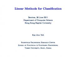
speakers, pronunciations, and instances. We want to determine if Sk can be modelled by a low-dimensional submanifold of IR1024 , and if such a submanifold could be characterised in a manner which would facilitate accurate statistical modelling of the data. We first applied a number of intrinsic dimension estimation techniques to the extracted sets Sk . Principal component analysis (PCA) was the first method considered, which assumes the data is contained in a linear subspace. The dimension of the subspace can be estimated by requiring that it should contain most of the average phoneme energy and we set this threshold at 90%. This PCA dimension estimate will be used as a reference to compare with three methods for non-linear dimension estimation. In particular we investigate estimators developed by Hein et al. [17], Costa et al. [18] and Takens [19] and applied them to the phomeme class data. Figure 1 shows the result of dimension estimation for six phonemes from different consonant groups. The findings here agree with the intuition that vowel-like phonemes should have a lower dimension than the fricatives. A typical dimension for a semivowel or a nasal phoneme, given these estimates, would be around 10; the case of /m/ is shown in Figure 1. For fricatives like /f/, the dimension is much higher. Given that the non-linear dimension estimates are mostly consistent and significantly lower than the PCA estimates we conclude that the phoneme distributions can be modelled as lowerdimensional non-linear manifolds. A number of techniques have recently been developed to find such non-linear manifold structures in data [20]. After an extensive study of the benefits and limitations of these methods, Isomap [15] and LLE [14][21] were selected for application to the phoneme dataset. They were considered especially suitable for the task having successfully found low-dimensional structure in images of human faces and handwritten digits in other studies. As explained above, although the methods can find structure, there is no straightforward way to apply noise adaptation if we were to use non-linearly reduced feature sets. We would therefore seek to identify the non-linear structures, and exploit them to constrain density models on the original linear feature space. As we now show, however, the dimensions of the nonlinear structures in our case are still too high for them to be learned accurately with the available quantity of data. Isomap is a method for finding a lower dimensional approximation of a dataset using geodesic distance estimates. Our initial comparison with PCA output showed that for a given embedding dimension the approximation provided by Isomap was better in terms of the L2 error [15] for our data. As in PCA we look for a step change in the spectrum of an appropriate Gram matrix to find the dimension estimate. However, this was not possible for the phoneme data as the spectra of the Gram matrices were smooth for all phonemes. We found similar results for LLE and suspected that in both cases the cause was undersampling of the manifold. These findings motivated the study of an artificial problem, to estimate how much data might be required to sufficiently sample the phoneme manifolds. The simple example of uniform probability distributions over hyperspheres with a given dimension was considered. A smooth histogram of pairwise distances among sampled points, in accordance with the theoretically expected form, then indicates a sufficient sampling of the uniform target distribution, whereas strong peaks – resulting from the fact that random vectors in high dimensional spaces are typically orthogonal to each other – suggest undersampling. Initially, when we set the dimension of the hypersphere to be comparable to that of the phoneme dimension estimates, and used a similar number of data points (∼ 1000), such peaks in the distance histograms were indeed present. When the dimension of the hypersphere was reduced to five, the peaks were smoothed out, suggesting that this five-dimensional manifold was
3
500 Intrinsic Correlation 450 Takens PCA (90%)
Dimension estimate
90
80
400
70
350
60
300
50
250
40
200
30
150
20
100
10
50
0
/b/
/f/
/m/
/r/
/t/
/z/
model. For the case of c mixture components this function has the form: c i h 1 X wi p(x) = (2) exp − (x − µi )T Σ−1 i (x − µi ) d 1 2 i=1 (2π) 2 |Σi | 2
PCA dimension estimate
100
0
Phoneme
Fig. 1. Intrinsic dimension estimates of example phoneme classes. The legend indicates the method of estimation. PCA estimates are plotted using the right hand scale
sufficiently sampled with a number of data points similar to the number of phoneme examples per class. In summary, the findings of the experiments suggest that if speech data manifolds exist in the acoustic waveform domain then they are under-sampled because of their relatively high intrinsic dimension. The number of required data points, n, could be expected to vary exponentially with the intrinsic dimensions, d, i.e. n ∼ αd for some constant α. In the hypersphere experiments α was approximately four, consequently the estimated quantity of data required to sufficiently sample a phoneme manifold with d ∼ 10 . . . 60 would be unrealistic, particularly at the upper end of this range. Given that the data-driven dimensionality reduction methods we have explored are not practical for the task considered, we now turn to more generic density models for the problem of phoneme classification in the presence of additive noise. In particular we will construct generative classifiers in the highdimensional space which do not attempt to exploit any submanifold structure directly. We will see that approximations are required, again due to the sparseness of the data, but also because of computational constraints. B. Generative Classification Generative classifiers use probability density estimates, p(x), learned for each class of the training data. The predicted class of a test point, x, is determined as the class k with the greatest likelihood evaluated at x. Typically the log-likelihood is used for the calculation; we denote the log-likelihood of x by L(x) = log(p(x)). Classification is performed using the following function: AL (x) = arg max L(k) (x) + log(πk ) k=1,...,K
(1)
where x can be predicted as belonging to one of K classes. The inclusion above of πk , the prior probability of class k, means that we are effectively maximising the log-posterior probability of class k given x. 1) Gaussian Mixture Models: Without assuming any additional prior knowledge about the phoneme distributions we use Gaussian mixture models (GMMs) to model phoneme densities. The models are trained using the expectation maximisation (EM) algorithm to maximise the likelihood of the training data for the relevant phoneme class. The training algorithm determines suitable parameters for the probability density function, p : Rd → R, of a Gaussian mixture
where wi , µi and Σi are the weight, mean vector and covariance matrix of the ith mixture component respectively. In the case of acoustic waveforms we additionally impose a zero mean constraint for models as a waveform x will be perceived the same as −x. With this constraint the corresponding models represent all information about the phoneme distributions in the covariance matrices and component weights. 2) Probabilistic Principal Component Analysis: In the preliminary experiments, we initially modelled the phoneme class densities using GMMs with full covariance matrices. However, it was not possible to accurately fit models with more than two components in the high dimensional space of acoustic waveforms, where d = 1024. Instead we considered using density estimates derived from mixtures of probabilistic principal component analysis (MPPCA) [10]. This method has a dimensionality reduction interpretation and produces a Gaussian mixture model where the covariance matrix of each component is regularised by replacement with a rank-q approximation: Σ = r 2 I + WWT
(3) √
Here the ith column of the d × q matrix W is given as λi vi corresponding to the ith eigenvalue, λi , and eigenvector, vi , of the empirical covariance matrix, with the eigenvalues arranged in descending order. The regularisation parameter r 2 is then taken as the mean of the remaining d − q eigenvalues: r2 =
d X 1 λi d − q i=q+1
(4)
3) Noise Adaptation: The primary concern of this paper is to investigate the performance of the trained classifiers in the presence of additive Gaussian noise. Generative classification is particularly suited for robust classification as the estimated density models can capture the distribution of the noise corrupted phonemes. As the noise is additive in the acoustic waveform domain, signal and noise models can be specified separately and then combined exactly by convolution. In the experiments of this section, phoneme data is normalised at the phoneme segment level with the SNR being specified relative to the segment rather than the whole sentence. This is clearly unrealistic as the mean energy of phonemes differs significantly between classes. However, it does provide a situation where each phoneme class is affected by the same local SNR. We can also think of this geometrically: for each phoneme class, the class density p(x) is blurred in the same way by convolution with an isotropic Gaussian of variance set by the SNR. The effect of the noise on classification then indirectly provides information on how well separated different phoneme classes are in the space of acoustic waveforms x. The white Gaussian noise model results in a covariance matrix that is a multiple of the identity matrix, σ 2 I, where σ 2 is the noise variance. We assume throughout that this is known, as it can be estimated reliably during periods without speech activity or using other techniques [22]. Hence the noise adaptation for the acoustic waveform representation is given ˜ 2 ): by replacing each covariance matrix Σ with Σ(σ 2 ˜ 2) = Σ + σ I Σ(σ (5) 1 + σ2 Speech waveforms are normalised to unit energy per sample. Clearly some normalisation of this type is needed to avoid adverse effects of irrelevant differences in speaker volume on classification performance, an issue that has been carefully studied in previous work [7].
4
C. Results of Exploratory Classification in PLP and Acoustic Waveform Domains In the exploratory study we consider only realisations of six phonemes (/b/, /f/, /m/, /r/, /t/, /z/) that were extracted from the TIMIT database [26]. This set includes examples from fricatives, nasals, semivowels and voiced and unvoiced stops. These classes provide pairwise discrimination tasks of a varying level of difficulty. For example /b/ vs. /t/ is a more challenging discrimination than /m/ vs. /z/. The phoneme examples are represented by the centre 64ms segment of the acoustic waveform corresponding to 1024 samples at 16kHz. Additionally the stops, /b/ and /t/ are aligned at the release point as prescribed by the given TIMIT segmentation. The data vectors are then normalised to have squared norm equal to the dimension of the segment corresponding to unit energy per sample as explained above. These initial experiments focus only on the centre of the phonemes to investigate the effectiveness of noise adaptation. As is well known, discrimination can be improved by considering the information provided by the transitions from one phonemes to the next. We will explore this in Section IV and see that it does indeed significantly help classification. Each phoneme class consists of approximately 1000 representatives, of which 80% were used for training and 20% for testing. The classification error bars, where indicated, were derived by considering five different such splits and give an indication of the significance of any differences in the accuracy of classifiers. A range of SNRs was chosen to explore classification errors all the way to chance level, i.e. 83.3% in the case of six classes. In total this gave six testing and training conditions; −18dB, −12dB, −6dB, 0dB, 6dB and quiet. At this exploratory stage only white Gaussian noise is considered. We use the same number of examples from each class, thus the prior probabilities πk are all equal to 1/6 and have no effect on predictions according to (1). For comparison the default 12th order PLP cepstra were computed for the 64ms segments. A sliding 25ms Hamming window was used with an overlap of 15ms leading to four frames of 13 coefficients [27]. These four frames were concatenated to give a PLP representation
90 80 70 60 Error [%]
The normalisation leads in the density models to covariance matrices Σ with trace d, the dimension of the data. Adding the noise as in the numerator of the equation above would give an average energy per sample of 1 + σ 2 . We also normalise noisy speech to unit energy per sample, and hence rescale the adapted covariance matrix by 1 + σ 2 as indicated above. There is no exact method for combining models of the training data with noise models in the case of MFCC and PLP features, as these representations involve non-linear transforms of the waveform data. Parallel model combination as proposed by Gales and Young [23] is an approximate approach for MFCC. A commonly used alternative method for adapting probabilistic models to additive noise is cepstral mean and variance normalisation (CMVN) [24], and we will consider this method in subsequent sections. At this exploratory stage, we study instead the matched condition scenario, where training and testing noise conditions are the same and a separate classifier is trained for each noise condition. In practice it would be difficult and computationally expensive to have a distinct classifier for every noise condition, in particular if noise of varying spectral shape is included in the test conditions. Matched conditions are nevertheless useful in our exploratory classification experiments: because training data comes directly from the desired noisy speech distribution, then assuming enough data is available to estimate class densities accurately this approach provides the optimal baseline for all noise adaptation methods [23],[25].
50 40 30
Quiet 6dB 0dB −6dB −12dB −18dB
20 10 0
−18
−12
−6 0 Test SNR [dB]
6
Quiet
Fig. 2. Error of PLP classifiers as a function of test SNR. Each curve shows the error of the classifier trained at the SNR indicated by the curve marker. The curves show the sensitivity of PLP classifiers when there is a mismatch between training and testing noise conditions. In particular the classifiers trained at 0dB and 6dB performs much worse when the test noise level is lower than the training level.
in R52 . The data was then standardised prior to training so that each of the 52 features had zero mean and unit variance across the entire training set that was considered. We discuss variants of this feature standardisation in Section III-A3. The PLP phoneme distributions were modelled using a single component PPCA mixture with a principal dimension of 40, i.e. c = 1 and q = 40; we experimented with other values but these parameters gave the best results. Figure 2 shows the test results for classifiers trained on data corrupted at the different noise levels. Each of the curves thus represents a different training SNR. It is clear that PLP classifiers are highly sensitive to mismatch between training and testing noise conditions. For example, when conditions are matched at 6dB SNR, the error is very low at 2.8%. However, if the same classifier is tested in quiet conditions this value increases significantly, to 53.7%. The analogous plot for waveform classifiers is shown in Figure 3, where the phoneme classes were modelled with c = 4 and q = 500. Acoustic waveform classifiers are less sensitive to mismatch between the assumed noise level to which they were adapted using (5), and the true testing conditions. Taking the classifier adapted to 6dB SNR as an example, we see that if assumed and true testing conditions are matched the error is 5.1% and when testing in quiet, it remains as low as 8.4%. Although the error for matched conditions is higher than that of PLP at this noise level, the increase due to mismatch is drastically reduced. We next consider the scenario where the true testing conditions are matched to those the models were trained in (PLP) or adapted to (waveforms). This is equivalent to taking the lower envelopes of Figures 2 and 3. In this case PLP gives a lower error rate than waveforms above 0dB SNR, while the opposite is true below this value. These results suggest that we should seek to combine the classification strengths of each representation, specifically the high accuracy of PLP classifiers at high SNRs and the robustness of acoustic waveform classifiers at all noise levels. Ideally this will result in a single combined classifier that only needs to be trained in quiet conditions and can be easily adapted to a range of noise conditions. To investigate this concept we consider the following
5
90
90
80
80
70
70
60
60
30
50
20
70 Combined Matched Combined Quiet
60 50
Error [%]
Error [%]
40
50 40 30
10 −18
0
−18
−12
−6
0
6
Quiet
30
Quiet 6dB 0dB −6dB −12dB −18dB
20
10 40
20 Combined Waveform PLP
10 −12
−6 0 Test SNR [dB]
6
0
Quiet
Fig. 3. Error of acoustic waveform classifiers as a function of test SNR. The curve marker indicates the assumed SNR to which the classifier was adapted using (5). The error rate is less sensitive to mismatch between the assumed and the true SNR when compared to the curves in Figure 2.
convex combination of the two log-likelihoods with each term being normalised by the relevant representation dimension. Let Lplp (x) and Lwave (x) be the log-likelihoods of a phoneme class, then the combined log-likelihood Lα (x) parameterised by α is given as: Lα (x) =
α (1 − α) Lwave (x) Lplp (x) + dplp dwave
(6)
where dplp = 52 and dwave = 1024 are the dimensions of the PLP and acoustic waveform representations, respectively. We would expect α to be almost zero for high SNRs and close to one for low SNRs in order to give the desired improvement in accuracy, and use this information to fit a combination function, α(σ 2 ). A suitable range of possible values of α was identified at each noise level from the condition that the error rate is no more than 2% above the error for the best α. This range is broad, so the particular form of the fitted combination function is not critical [28]. We choose the following sigmoid function with two parameters σ02 and β: α(σ 2 ) =
1 2
1 + eβ(σ0 −σ
2)
(7)
A fit through the numerically determined suitable ranges of α then gives σ02 = 11dB, β = 0.3. We also consider combinations involving PLP classifiers trained in quiet conditions and adapted to noise using CMVN, where a similar fit gives σ02 = 11dB, β = 0.7. The above combination in (6) is equivalent to using multiple streams of features, one consisting of the waveform and the other of the PLP features derived from the same waveform segment. Data fusion at the feature level that concatenates the vectors of features from each source would be an alternative method of combining the two representations. However, such a method would not be suitable for the combination of PLP and acoustic waveforms, predominantly because the contribution to the resulting likelihood from each representation is approximately proportional to the feature space dimension. Hence the likelihood contribution from the acoustic waveform portion of the fused vector would dominate. Figure 4 shows the result of the combination, when the acoustic waveform classifiers are trained in quiet conditions and then adapted to noise according to (5), while the PLP classifiers are trained under matched conditions. We see in the main plot that the combined
−18
−12
−6 0 Test SNR [dB]
6
Quiet
Fig. 4. Performance of the combined classifier when PLP models trained under matched conditions are used. The combined classifier is uniformly at least as accurate as those it is derived from and gives significant improvement around −6dB SNR. Inset: Comparison with the combined classifier trained only in quiet conditions.
classifier has uniformly lower error rate across the full range of noise conditions. In particular, around −6dB SNR the combination performs significantly better than either of the underlying classifiers. This is interesting because it means that the combination achieves more than a hard switch between PLP and waveform classifiers could. The inset shows a comparison of combined classifiers involving PLP trained in matched conditions and PLP trained in quiet and adapted using CMVN respectively. These two approaches to PLP training should represent the extremes of performance, with noise adaptation techniques more advanced than CMVN expected to lie in between. Encouragingly, the inset to Figure 4 shows that by an appropriate combination with waveform classifiers the performance gap between having only PLP models trained in quiet conditions and those trained in matched conditions is dramatically reduced. D. Conclusions of Exploratory Data Analysis The exploratory data analysis shows that acoustic waveform classifiers, which can be exactly adapted to noise when the noise conditions are known, are also more robust to mismatch between assumed and true testing conditions. The combined classifier retains the accuracy of PLP in quiet conditions whilst simultaneously providing the robustness of acoustic waveforms in the presence of noise. In order to confirm these conclusions a more realistic test is required. As described above, we also found that the best model fits were obtained with only a small number of mixture components, whether using full covariance matrices or more restricted density models in the form of MPPCA. In both cases too many model parameters are required to specify each mixture component, meaning that mixtures with many components cannot be learned reliably from limited data. In the next section, the issue of parameter count reduction will be even more acute as many of the phoneme classes have even fewer examples than those considered so far. The problem will be addressed by using diagonal covariance matrices in the GMMs, with the data appropriately rotated into a basis which approximately decorrelates the data. Additionally the SNRs will be specified at sentence level which can cause local SNR mismatch and will provide a more challenging test of the robustness of the classifiers. We will also investigate the length of the segments used to represent the phonemes.
6
This is particularly relevant when comparing the acoustic waveform classifiers to those of PLP+∆+∆∆ as the deltas use information from neighbouring frames. It will be shown that by optimising the numbers of frames for each representation we get a similar benefit for phoneme classification as when using deltas. Finally we will show the effect of including information from the whole phoneme rather than just the frames from the centre. III. F IXED D URATION R EPRESENTATION WITH R EFINED M ODELS In this section we consider how to enhance the generative models so that they can deal with more realistic classification tasks. All previous experiments are now repeated on the standard TIMIT benchmark [29] with noise added so that the SNR is specified at sentence level. This means that the local SNR of the phoneme segments can differ significantly from the sentence level value. There is a large variation in the size of the phoneme classes hence those relative frequencies have a greater effect as the prior in (1). We also consider model averaging, which removes the need to select the number of components in mixture models. A. Model Refinements 1) Diagonal Covariance Matrices: We observed in the preliminary exploration that even PPCA requires an excessive number of parameters compared to the quantity of available data. Hence, GMMs with diagonal covariance matrices are used for all following experiments. This is a common modelling approximation when training data is sparse. Diagonal covariances matrices will be a good approximation provided the data is presented in a basis where correlations between features are weak. For the acoustic waveform representation, this is clearly not the case on account of the strong temporal correlations in speech waveforms. We therefore systematically investigated candidate low-correlation bases derived from PCA, wavelet transforms and DCTs. Although the optimal basis for decorrelation on the training set is indeed formed by the phoneme-specific principal components, we found that the lowest test error is in fact achieved with a DCT basis. The density model used for the phoneme classes in the acoustic waveform domain now becomes: c X
wi
i h 1 exp − (x − µi )T CT D−1 i C(x − µi ) 2 i=1 (2π) |D | (8) where wi , µi and Di are the weight, mean vector and diagonal covariance matrix of the ith mixture component respectively. C is an orthogonal transformation selected to decorrelate the data at least approximately. In the case of acoustic waveforms we choose C to be a DCT matrix, as explained above. Preliminary experiments showed that, instead of performing a single DCT on an entire phoneme segment, it is advantageous to separate DCTs in non-overlapping subsegments of length 10ms, mirroring (except for the lack of overlaps) the frame decomposition of MFCC and PLP. For a sampling rate of 16kHz as in our data, the transformation matrix C is then block diagonal consisting of 160 × 160 DCT blocks. For the MFCC and PLP representations we choose C to be the identity matrix as they already involve some form of DCT and the features are approximately decorrelated. 2) Model Average: In general, more variability of the training data can be captured with an increased number of mixture components; however, if too many components are used over-fitting will occur. The best compromise is usually located by cross validation using the classification error on a development set. The result is a single value for the number of components required. We use an alternative approach and take the model average over the number of components, p(x) =
d 2
1 i 2
effectively a mixture of mixtures [30]. We start from a selection of models parameterised by the number of components, c, which takes values in C = {1, 2, 4, 8, 16, 32, 64, 128} or subsets of it. The entries in this set are uniformly distributed on a log scale to give a good range of model complexity without including too many of the complex models. We compute the model average log-likelihood M(x) as: X � uc exp(Lc (x)) (9) M(x) = log c∈C
1 |C|
with the model weights uc = and Lc (x) being the log-likelihood of x given the c-component model. Alternatively the mixture weights allocated to each model could be determined from the posterior densities of the models on a development set to give a class dependent weighting, i.e. P exp(Lc (x)) P uc = P x∈D (10) d∈C x∈D exp(Ld (x)) where D is a development set. Preliminary experiments suggested that using those posterior weights only gives a slight improvement 1 over (9). We therefore adopt those uniform weights (uc = |C| ) for all results shown in this paper. 3) Noise adaptation for sentence-normalised data: Now we consider the more realistic case where the SNR is only known at sentence-level. All sentences will therefore be normalised to have unit energy per sample in quiet and noisy conditions. Different phonemes within these sentences can have higher or lower energies, as reflected in the density models by covariance D with trace above or below d, where d is the dimension of the feature vectors. The relative energy of each phoneme class, which we had discarded in Section II-C, can thus be used during classification. The adaptation to noise has the same form as in (5): 2 ˜ 2) = D + σ N D(σ 1 + σ2
(11)
where N is the covariance matrix of the noise transformed by C, normalised to have trace d. For white noise, N is the identity matrix, otherwise it is estimated empirically from noise samples. In general a full covariance matrix will be required to specify the noise structure. However, with a suitable choice of C the resulting N will be close to diagonal, and indeed when C is a segmented DCT we find this to be true in our experiments with pink noise. To avoid the significant computational overheads of introducing non-diagonal matrices, we therefore retain only the diagonal elements of N. The normalisation by 1+σ 2 arises as before: on average, a clean sentence to which noise has been added has energy 1 + σ 2 per sample and the normalisation to unit energy of both clean and noisy data requires dividing all covariances by this factor. In contrast to our exploratory study in ˜ Section II, and because of the varying local SNR, the traces of D and D are then no longer necessarily equal. We now consider noise compensation techniques for MFCC and PLP features. As mentioned above, cepstral mean and variance normalisation (CMVN) [24] is an approach commonly used in practice to compensate noise corrupted features. This method requires estimates of the mean and variance of the features, usually calculated sentencewise on the test data or with a moving average over a similar time window. We take this to be a realistic baseline. Alternatively the required statistics can be estimated from a training set that has been corrupted by the same type and level of noise as used in testing. (For large data sets, these statistics should be essentially the same as on the noisy test set, barring systematic effects from e.g. different training and test speakers.) Clearly both approaches have merit. For example, sentence level CMVN requires no direct knowledge of the test conditions, and can remove speaker specific variation from the
7
65 PLP (Standardised) PLP+∆+∆∆ (Standardised) PLP (Sentence) PLP+∆+∆∆ (Sentence)
90 80
Waveform MFCC PLP MFCC+∆+∆∆ PLP+∆+∆∆ Individual models Component average
60 55
70
Error [%]
Error [%]
50 60 50
40
40
35
30 20
45
30
−18
−12
−6
0
6 12 SNR [dB]
18
24
30
//
Quiet
Fig. 5. Comparison of sentence level cepstral mean and variance normalisation (dashed) and training set (solid) standardisation for PLP and PLP+∆+∆∆.
data. The estimates will be less accurate and as a consequence it is difficult to standardise all components in long feature vectors obtained by concatenating frames; instead, we standardise frame by frame. Using a noisy training set for CMVN requires that the test conditions are known so that either data can be collected or generated for training under the same conditions. The feature means and variances can be obtained accurately, and in particular we can standardise longer feature vectors. However, as the same standardisation is used for all sentences, any variation due to individual speakers will persist. A comparison of the two standardisation techniques is shown in Figure 5. Curves are displayed for both methods, using PLP features with and without ∆+∆∆. Standardisation on the noisy training set gives lower error rates both in quiet conditions and in noise, hence all results for CMVN given below use this method. B. Experimental setup Realisations of phonemes were extracted from the SI and SX sentences of the TIMIT [26] database. The training set consists of 3,696 sentences sampled at 16kHz. Noisy data is generated by applying additive Gaussian noise at nine SNRs. Recall that the SNRs were set at the sentence level, therefore the local SNR of the individual phonemes may differ significantly from the set value, causing mismatch in the classifiers. In total ten testing and training conditions were run; −18dB to 30dB in 6dB increments and quiet (Q). Following the extraction of the phonemes there are a total of 140,225 phoneme realisations. The glottal closures are removed and the remaining classes are then combined into 48 groups in accordance with [29], [31]. Even after this combination some of the resulting groups have too few realisations. The smallest groups with fewer than 1,500 realisations were increased in size by the addition of temporally shifted versions of the data. i.e. if x is an example in one of the small training classes then the phoneme segments extracted from positions shifted by k = −100, −75, −50, . . . , 75, 100 samples were also included for training. This increase in the size of the smaller training classes ensures that the training procedure is stable. For the purposes of calculating error rates, some very similar phoneme groups are further regarded as identical, resulting in 39 groups of effectively distinguishable phonemes [29]. PLP features are obtained in the standard manner from frames of width 25ms, with a shift of 10ms between neighbouring frames and correspondingly an
25
1
2
4 8 16 Number of Components
32
64
Fig. 6. Model averaging for acoustic waveforms, MFCC and PLP models, all trained and tested in quiet conditions. Solid: GMMs with number of components shown; dashed: average over models up to number of components shown. The model average reduces the error rate in all cases.
overlap of 15ms. We also include now in our comparisons MFCC features. Standard implementations [27] of MFCC and PLP with default parameter values are used to produce a 13-dimensional feature vector from each time frame. The inclusion of ∆ + ∆∆ increases the dimension to 39. Our exploratory results in Section II gave successful classification for acoustic waveforms using a 64ms window. For the MFCC and PLP representations, we therefore consider the five frames closest to the centre of each phoneme, covering 65ms, and concatenate their feature vectors. Results are shown for the representations with and those without ∆ + ∆∆ , giving feature vector dimensions of 5 × 39 = 195 and 5 × 13 = 65, respectively. The acoustic waveform representation is obtained by dividing each sentence into a sequence of 10ms non-overlapping frames, and then taking the seven frames (70ms) closest to the centre of each phoneme, resulting in a 1120dimensional feature vector. Each frame is individually processed using the 160-point DCT. We present results for white and pink noise and will see that the approximation using diagonal covariances D in the DCT basis is sufficient to give good performance. The impact of the number of frames included in the MFCC, PLP and acoustic waveform representations is investigated in the next section. C. Results Gaussian mixture models were trained with up to 64 components for all representations. We comment briefly on the results for individual mixtures, i.e. with a fixed number of components. Typically performance on quiet data improved with the number of components, although this has significant cost for both training and testing. The optimal number of components for MFCC and PLP models in quiet conditions was 64, the maximum considered here. However, in the presence of noise the lowest error rates were obtained with few components; typically there was no improvement beyond four components. As explained in Section III-A2, rather than working with models with fixed numbers of components, we average over models, i.e. over the number of mixture components, in all the results reported below. Figure 6 shows that the improvement obtained by this in quiet conditions is approximately 2% for both acoustic waveforms and PLP
8
100
with a small improvement seen for MFCC also. The model average similarly improved results in noise and this will be discussed further in the next section.
The same experiment was repeated using pink noise extracted from the NOISEX-92 database [32]. The results for both noise types were similar for the waveforms classifiers. For PLP+∆+∆∆, adapted to noise using CMVN, there is a larger difference between the two noise types, with pink noise leading to lower errors. Nevertheless, the better performance is achieved by acoustic waveforms below 18dB SNR. Results for GMM classification on the TIMIT benchmark in quiet conditions have previously been reported in [31], [33] with errors of 25.9% and 26.3% respectively. To ensure that our baseline is valid we compared our experiment in quiet conditions for PLP+∆+∆∆ and obtained a comparable error rate of 26.3% as indicated in the bottom right corner of Figure 7. Following these encouraging results we seek to explore the effect of optimising the number of frames and the inclusion of information from the entire phoneme. The expectation is that including more frames in the concatenation for acoustic waveforms will have a similar effect to adding ∆+∆∆ for MFCC and PLP. A direct analogue of deltas is unlikely to be useful for waveforms: MFCC and PLP are based on log magnitude spectra that change little during stationary phonemes, so that local averaging or differencing is meaningful. For waveforms, where we effectively retain not just Fourier component amplitudes but also phases, these phases combine essentially randomly during averaging or differencing, rendering the resulting delta-like features useless.
80 70 Error [%]
One set of key results comparing the error rates in noise for phoneme classification in the three domains is shown in Figure 7. The MFCC and PLP classifiers are adapted to noise using CMVN. This method is comparable with the adapted waveform models as it only relies on the models trained in quiet conditions. The curve for acoustic waveforms is for models trained in quiet conditions and then adapted to the appropriate noise level using (11). Comparing waveforms first to MFCC and PLP without ∆+∆∆, we see that in quiet conditions the PLP representation gives the lowest error. The error rates for MFCC and PLP are significantly worse in the presence of noise, however, with acoustic waveforms giving an absolute reduction in error at 0dB SNR of 40.6% and 41.9% compared to MFCC and PLP respectively. These results strengthen the case that the adaptability of acoustic waveform models gives them a definite advantage in the presence of noise with the crossover point occurring above 30dB SNR. Curves are also shown for MFCC+∆+∆∆ and PLP+∆+∆∆. Again the same trend holds; performance is good in quiet conditions but quickly deteriorates as the SNR decreases. The crossover point is around 24dB for both representations. The chance-level error rate of 93.5% can be seen below 0dB SNR for the MFCC and PLP representations without deltas and below 6dB SNR when deltas are included, whereas the acoustic waveform classifier performs significantly better than chance with an error of 76.7% even at −18dB SNR. The dashed curves in Figure 7 represent the error rates obtained for classifiers trained in matched conditions with and without ∆+∆∆. The results show that the waveform classifier compares favourably to MFCC and PLP below 24dB SNR when no deltas are appended. Including ∆+∆∆ does reduce the error rates significantly and the crossover then occurs between 0dB and 6dB SNR. It is these observations that mainly motivate our further models development below: clearly we should aim to include information similar to deltas in the waveform representation.
90
60 50 Waveform MFCC PLP MFCC+∆+∆∆ PLP+∆+∆∆
40 30 20
−18
−12
−6
0
6 12 18 Test SNR [dB]
24
30
//
Q
Fig. 7. Comparison of adapted acoustic waveform classifiers with MFCC and PLP classifiers trained in quiet conditions adapted by feature standardisation. All classifiers use the model average of mixtures up to 64 components. Dotted line indicates chance level at 93.5%. When the SNR is less that 24dB, acoustic waveforms are the significantly better representation, with an error rate below chance even at -18dB SNR. Dashed curves show results of matched training for corresponding MFCC and PLP representations.
IV. S EGMENT D URATION , VARIABLE D URATION P HONEME M APPING AND C LASSIFIER C OMBINATION A. Segment Duration Ideally all relevant information should be retained by our phoneme representation, but as it is difficult to determine exactly which information is relevant we initially choose to take f consecutive frames closest to the centre of each phoneme and concatenate them. Whilst the precise number of frames required for accurate classification could in principle be inferred from the statistics of the phoneme segment durations, we see in Table I that those durations not only vary significantly between classes but also that the standard deviation within each class is at least 24ms. Therefore no single length can be suitable for all classes. The determination of an optimal f from the data statistics would be even more more complicated when ∆+∆∆ are included, because these incorporate additional information about the dynamics of the signal outside the f frames. Assuming that no single value of f will be optimal for all phoneme classes we instead consider the sum of the mixture log-likelihoods Mf , as defined in (9) but now indexed by the number of frames used. The sum is taken over the set F which contains the values of f with the lowest corresponding error rate, for example F = {7, 9, 11, 13, 15} for PLP: X Mf (xf ) (12) R(¯ x) = f ∈F
where x ¯ = {xf |f ∈ F}, with xf being the vector with f frames. Note that we are adding the log-likelihoods for different f , which amounts to assuming independence between the different xf in x ¯. Clearly this an imperfect model, as e.g. all components of x7 are also contained in x11 and so are fully correlated, but our experiments show that it is useful in practice. We also implemented the alternative of concatenating the xf into one longer feature vector and then training a joint model on this, but the potential benefits of accounting for correlations are far outweighed by the disadvantages of having to fit density models in higher dimensional spaces. Consistent with the independence assumption in (12), in noise we adapt the models Mf
9
40ms
where x ¯s = {xfs |f ∈ F} with xfs being the vector with f frames ˆ centred on sector s, and x ¯ gathers all x ¯s . Given the functions derived above, the class of a test point can be predicted using one of the following:
40ms 30%
40%
/t/
30%
/ay/
/f/
(k)
time 15% A f frames XA
35% B
f frames X
35% C f frames XC
f frames X
B
E f frames XE
(k)
D
TABLE I Duration statistics [ms] of the training data grouped by broad phonetic class. Group
Min
Mean ± std.
Max
Vowels
2.2
86.0 ± 46.7
438.6
7.6
54.5 ± 25.6
260.6
Strong Fricatives
14.9
99.5 ± 38.9
381.2
Weak Fricatives
4.5
68.2 ± 37.3
310.0
Stops
2.9
39.3 ± 24.0
193.8
Silence
2.0
94.9 ± 107.5
2396.6
All
2.0
79.4 ± 63.4
2396.6
B. Sector sum Although phonemes vary in duration, GMMs require data that has a consistent dimension. We next establish a method to map the variable length phoneme segments to a fixed length representation for classification. In the previous subsection only frames from the centre of the phoneme segments were used to represent a phoneme. We extend that centre-only concatenation to use information from the entire segment by taking f frames with centres closest to each of the time instants A,B,C,D and E that are distributed along the duration of the phoneme as shown in Figure 8. In this manner the representation consists of five sequences of f frames per phoneme. Those sets of frames are then concatenated to give five vectors xA , xB , xC , xD and xE . We train five models on those sectors and then combine the information they provide about each sector, again assuming independence by taking the sum of the log-likelihoods of the sectors: X
s∈{A,B,C,D,E}
Ms (xs )
(13)
where x ˆ = {xA , xB , xC , xD , xE } and Ms denotes the model for sector s, using some fixed number of frames f . Both improvements can be combined by taking the sum of the f -averaged log-likelihoods, Rs (¯ xs ), over the five sectors s: X ˆ Rs (¯ xs ) (14) T (x ¯) = s∈{A,B,C,D,E}
(16)
AS x) = arg max Sf (ˆ x) + log(πk ) f (ˆ
(17)
ˆ ˆ AT (x ¯) = arg max T (k) (x ¯) + log(πk )
(18)
k=1,...,K
separately and then combine them as above. The same applies to the further combinations discussed next.
S(ˆ x) =
AR (¯ x) = arg max R(k) (¯ x) + log(πk ) k=1,...,K
Fig. 8. Comparison of phoneme representations. Top: Division described in [33] resulting in five sectors, three covering the duration of the phoneme and two of 40ms duration around the transitions. Bottom: f frames closest to the five points A, B, C, D and E (which correspond to the centres of the regions above) are selected to map the phoneme segment to five feature vectors xA , xB , xC , xD and xE .
Nasals
(15)
k=1,...,K
15% D
AM f (x) = arg max Mf (x) + log(πk )
k=1,...,K
where πk is the prior probability of predicting class k as in (1). C. Results Figure 9 shows the impact of the number of frames concatenated from each sector on the classification error, focusing on quiet conditions. We see that the best results for acoustic waveform classifiers are achieved around 9 frames, and around 11 frames for PLP without deltas. The PLP+∆+∆∆ features are less sensitive to the number of frames with little difference in error from 1 to 13 frames. We can now also assess quantitatively the performance benefit of including the deltas. If we consider the best results obtained for PLP without deltas, 22.4% using 11 frames, with the best for PLP+∆+∆∆, 21.8% with 7 frames, then the performance gap of 0.6% is much smaller than if we were to compare error rates where both classifiers used the same number of frames. Clearly it is not surprising that fewer PLP+∆+∆∆ frames are required for the same level of performance as the deltas are a direct function of the neighbouring PLP frames. It is still worth noting that in terms of the ultimate performance on this classification task the error rates with and without deltas are similar. The results discussed above are directly comparable with the GMM baseline results from other studies, shown in Table III. The error rates obtained using the f -average over the five best values of f are 32.1%, 21.4% and 18.5% for acoustic waveforms, PLP and PLP+∆+∆∆ respectively. Table II shows the absolute percentage error reduction for each of the four classifiers (15)–(18) in quiet conditions, compared to the GMM with the single best number of mixture components and number of frames f . The relative benefits of the f -average and the sector sum are clear. The sector sum gives the bigger improvements on its own in all cases compared to only the f -average, but the combination of the two methods is better still throughout. The same qualitative trend holds true in noise. Figure 10 compares the performance of the final classifiers, including both the f -average and the sector sum, on data corrupted by pink noise. The solid curves give the results for the acoustic waveform classifier adapted to noise using (11), and for the PLP classifier with and without ∆+∆∆ trained in quiet conditions and adapted to noise by CMVN. The errors are generally significantly lower than in Figure 7, showing the benefits of f -averaging and the sector sum. PLP+∆+∆∆ remains the better representation for very low noise, but waveforms give lower errors beyond a crossover point between 12dB and 18dB SNR, depending on whether we compare to PLP with or without ∆+∆∆. As before, they also perform better than chance down to −18dB SNR. The dashed lines in Figure 10 show for comparison the performance of PLP classifiers trained in matched conditions. As explained, the CMVN and matched curves for PLP provide the extremes between which we would expect a PLP classifier to perform if model adaption analogous to that used with the acoustic waveforms was possible, or some other method to improve robustness was
10
TABLE III Existing error rates obtained in other studies for a range of classification methods on the TIMIT core test set. Results in this paper are most comparable to the GMM baselines.
60 Waveform PLP PLP+∆+∆∆ Model avg. Sector sum
55 50
Method
31.4
GMM baseline [33]
26.3
GMM baseline [36]
24.1
GMM baseline [37]
23.4
GMM (f -average + sector sum) PLP+∆+∆∆
18.5
30
SVM, 5th order polynomial kernel [33]
22.4
25
Large Margin GMM (LMGMM) [31]
21.1
Regularized least squares [37]
20.9
Hidden conditional random fields [38]
20.8
Hierarchical LMGMM H(2,4) [36]
18.7
Optimum-transformed HMM with context (THMM) [35]
17.8
Committee hierarchical LMGMM H(2,4) [36]
16.7
45 Error [%]
Error [%]
HMM (Minimum Classification Error) [35]
40 35
20 15
1
3
5
7 9 Number of frames
11
13
15
Fig. 9. Error rates of the different representations in quiet conditions, as a function of f , the number of frames considered. Dashed: prediction (15) using only the central sector. Dotted: prediction (16) using the sum over all five sectors, leading to a clear improvement in all cases.
employed such as the ETSI advanced front-end (AFE) [34]. As expected, the matched conditions PLP+∆+∆∆ classifier has the best performance for all SNR. However, in noise the adapted acoustic waveform classifier is significantly closer to matched PLP+∆+∆∆ than PLP+∆+∆∆ with CMVN.
of α = 0.003. When noise is present the combined classifier is at least as accurate as the acoustic waveform classifier, and significantly better around 18dB SNR. The combined classifier does improve upon PLP+∆+∆∆ classifiers trained in matched conditions at very low SNR and narrows the performance gap to the order of no more than 9% throughout, rather than 22% when comparing to PLP+∆+∆∆ adapted by CMVN. V. C ONCLUSION & D ISCUSSION
TABLE II Absolute reduction in percentage error for each of the classifiers (15)–(18) in quiet conditions. Model
Waveform
PLP
PLP+∆+∆∆
Model average (AM )
1.6
2.8
4.4
f -average (AR )
5.6
6.0
6.3
Sector sum (AS )
6.7
8.4
8.7
f -average + sector sum (AT )
9.9
10.0
10.4
D. Combination of PLP and Acoustic Waveform Classifiers We see from the results shown so far that, as in the preliminary experiments, PLP performs best in quiet conditions with acoustic waveforms being more robust to additive noise. To gain the benefits of both representations, we propose to merge them via a linear combination of the corresponding log-likelihoods, parameterised by a coefficient α: Tα (x) = (1 − α)Tplp (x) + αTwave (x)
(19)
where Tplp (x) and Twave (x) are the log-likelihoods of a point x. Tα (x) is then used in place of T (x) in (18) to predict the class. The combination differs from (6) as the effect of the prior class probabilities is more relevant now and the absolute log-likelihoods must be used rather than the scaled quantities. This is again equivalent to a multistream model, where each sector and value of f is an independent stream. A noise-dependent α(σ 2 ) is determined as explained in Section II-C, giving parameter values (σ 2 = 17dB, β = 0.3) in (7). The error of the combined classifier using models trained in quiet conditions is shown as the dash-dotted curve in Figure 10. In quiet conditions the combined classifier is slightly more accurate (18.4%) than PLP+∆+∆∆ alone, corresponding to a small value
In this paper we have studied some of the potential benefits of phoneme classification in linear feature domains directly related to the acoustic waveform, with the aim of implementing exact noise adaptation of the resulting density models. In Section II we outlined the results of our exploratory data analysis, where we found intrinsic nonlinear dimension estimates lower than linear dimension estimates from PCA. That observation suggested that it should be possible to construct low dimensional embeddings to be used later with generative classifiers. However, existing techniques failed to find enough structure in the phoneme dataset as it is too sparse to accurately define the embeddings. Consequently we used GMMs to model the phoneme distributions in acoustic waveform and PLP domains. Additionally, a combined classifier was used to incorporate the performance of PLP in quiet conditions with the noise robustness of acoustic waveforms. Given the encouraging results from these experiments on a small set of phonemes we progressed to a more realistic task and extended the classification problem to include all phonemes from the TIMIT database. This gave results that could be directly compared to the existing results in Table III, classifiers representing current progress on the TIMIT benchmark. All of the entries show the error for isolated phoneme classification except for the optimum-transformed HMM (THMM) [35] that uses context information derived from continuous speech. The inclusion of context for the HMM classifiers reduces the error rate from 31.4% to 17.8%. This dramatic reduction suggests that if the other classifiers were also developed to directly incorporate contextual information, significant improvements could be expected. We used the standard approximation of diagonal covariance matrices to reduce the number of parameters required to specify the GMMs. The issue of selecting the number of components in the mixture models was approached by taking the model average with respect to the number of components for a sufficiently large set of values. The results supported our earlier conclusions, but also
11
Waveform PLP (Standardised) PLP+∆+∆∆ (Standardised) PLP (Matched) PLP+∆+∆∆ (Matched) Combined(∆+∆∆)
90 80
Error [%]
70 60 50 40 30 20 −18
−12
−6
0
6 12 SNR [dB]
18
24
30
//
Quiet
Fig. 10. Performance of the classifiers in pink noise. Curves are shown for the best representation from Fig. 9 using both the f -average and sector sum. Dash-dotted line: Combined waveform and PLP+∆+∆∆ classifier, with the latter adapted to noise by feature standarisation using CMVN.
illustrated that waveforms are potentially lacking the significant benefits obtained by ∆+∆∆ features. This motivated us to further improve the classifiers by using multiple segment durations and then taking the sum of the log-likelihoods. Information from the whole phoneme was included by repeating the process centred at five points in the phoneme. The best practical classifiers in this paper were obtained using the combination of acoustic waveforms with PLP+∆+∆∆. We expect that the results can be further improved by including techniques considered by other authors, in particular, committee classifiers and the use of a hierarchy to reduce broad phoneme class confusions [36],[39]. The models could be developed to explicitly model correlations between feature vectors obtained for different number of frames f and also between feature vectors from different sectors, provided sufficient data was available. Additionally, weighting the sector sum and frame average or allowing the number of frames to be different for each sector could be investigated. Finally, given the qualitative similarity between features from different sectors, and features as they would be emitted by different states in HMMs, it would also be of interest to explore the linear feature sets used here in the context of continuous speech recognition. R EFERENCES [1] G. Miller and P. Nicely, “An Analysis of Perceptual Confusions among some English Consonants,” J. Acoust. Soc. Am., vol. 27, pp. 338–352, 1955. [2] R. Lippmann, “Speech Recognition by Machines and Humans,” Speech Comm., vol. 22, no. 1, pp. 1–15, 1997. [3] J. Sroka and L. Braida, “Human and Machine Consonant Recognition,” Speech Comm., vol. 45, no. 4, pp. 401–423, 2005. [4] H. Hermansky, “Perceptual Linear Predictive (PLP) Analysis of Speech,” J. Acoust. Soc. Am., vol. 87, no. 4, pp. 1738–1752, 1990. [5] A. Poritz, “Linear Predictive Hidden Markov Models and the Speech Signal,” in Proc. ICASSP, 1982. [6] Y. Ephraim and W. Roberts, “Revisting Autoregressive Hidden Markov Modeling of Speech Signals,” in IEEE Signal Processing Letters, vol. 12, no. 2, Feb. 2005, pp. 166–169. [7] H. Sheikhzadeh and L. Deng, “Waveform-Based Speech Recognition Using Hidden Filter Models: Parameter Selection and Sensitivity to Power Normalization,” IEEE Trans. Speech and Audio Processing, vol. 2, no. 1, pp. 80 –89, Jan 1994.
[8] B. Mesot and D. Barber, “Switching Linear Dynamical Systems for Noise Robust Speech Recognition,” IEEE Trans. Audio, Speech and Language Processing, vol. 15, no. 6, pp. 1850–1858, 2007. [9] R. E. Turner and M. Sahani, “Modeling Natural Sounds with Modulation Cascade Processes,” in Advances in Neural Information Processing Systems, vol. 20, 2008. [10] M. Tipping and C. Bishop, “Mixtures of Probabilistic Principal Component Analysers,” Neural Computation, vol. 11, no. 2, pp. 443–482, 1999. [11] N. Vasiloglou and A. G. D. Anderson, “Learning the Intrinsic Dimensions of the TIMIT Speech Database with Maximum Variance Unfolding,” in IEEE Workshops on DSP and SPE, 2009. [12] S. Zhang and Z. Zhao, “Dimensionality Reduction-based Phoneme Recognition,” in Proc. ICSP, 2008. [13] T. Hastie, R. Tibshirani, and J. Friedman, The Elements of Statistical Learning: Data Mining, Inference, and Prediction., 2009. [14] S. Roweis and L. Saul, “Nonlinear Dimensionality Reduction by Locally Linear Embedding,” Science, vol. 290, pp. 2323–2326, 2000. [15] L. Saul, K. Weinberger, J. Ham, F. Sha, and D. Lee, “Spectral Methods for Dimensionality Reduction,” in Semisupervised Learning. Cambridge, MA: MIT Press, 2006. [16] N. Lawrence, “Probabilistic Non-Linear Principal Component Analysis with Gaussian Process Latent Variable Models,” J. Mach. Learn. Res., vol. 6, pp. 1783 –1816, 2005. [17] M. Hein and J.-Y. Audibert, “Intrinsic Dimensionality Estimation of Submanifolds in Rd ,” in Proc. ICML, vol. 119, 2005, pp. 289–296. [18] J. Costa and A. Hero, “Geodesic Entropic Graphs for Dimension and Entropy Estimation in Manifold Learning,” IEEE Trans. on Signal Processing, vol. 52, no. 8, pp. 2210–2221, 2004. [19] F. Takens, “On the Numerical Determination of the Dimension of an Attractor,” in Lecture notes in mathematics. Dynamical systems and bifurcations, vol. 1125. Springer, 1985, p. 99. [20] L. van der Maaten, E. Postma, and H. van den Herik, “Dimensionality reduction: A comparative review,” 2007. [21] S. Roweis, L. Saul, and G. Hinton, “Global Coordination of Local Linear Models,” Advances in Neural Information Processing Systems, vol. 14, 2002. [22] C. Kim and R. Stern, “Robust Signal-to-Noise Ratio Estimation Based on Waveform Amplitude Distribution Analysis,” in Proc. Interspeech, 2008. [23] M. Gales and S. Young, “Robust continuous speech recognition using parallel model combination,” IEEE Trans. on Speech and Audio Processing, vol. 4, pp. 352–359, 1996. [24] P. Jain and H. Hermansky, “Improved Mean and Variance Normalization for Robust Speech Recognition,” in Proc. ICASSP, 2001. [25] R. Rose, “Environmental Robustness in Automatic Speech Recognition,” Robust2004 - ISCA and COST278 Workshop on Robustness in Conversational Interaction, 2004. [26] J. Garofolo, L. Lamel, W. Fisher, J. Fiscus, and D. Pallett, The DARPA TIMIT acoustic-phonetic continous speech corpus. NIST. Philiadelphia: Linguistic Data Consortium, 1993. [27] D. Ellis, “PLP and RASTA (and MFCC, and inversion) in Matlab,” 2005, online web resource, http://labrosa.ee.columbia.edu/matlab/rastamat/. [28] M. Ager, Z. Cvetkovi´c, P. Sollich, and B. Yu, “Towards Robust Phoneme Classification: Augmentation of PLP Models with Acoustic Waveforms,” in Proc. EUSIPCO, 2008. [29] K.-F. Lee and H.-W. Hon, “Speaker-Independent Phone Recognition using Hidden Markov Models,” IEEE Trans. Acoustics, Speech and Signal Processing, vol. 37, no. 11, pp. 1641–1648, 1989. [30] S. Srivastava, M. Gupta, and B. Frigyik, “Bayesian Quadratic Discriminant Analysis,” Journal of Machine Learning Research, vol. 8, pp. 1287– 1314, 2007. [31] F. Sha and L. Saul, “Large Margin Gaussian Mixture Modeling for Phonetic Classification and Recognition,” in Proc. ICASSP, 2006. [32] A. Varga, H. Steeneken, M. Tomlinson, and D. Jones, “The NOISEX-92 study on the effect of additive noise on automatic speech recognition,” DRA Speech Research Unit, Tech. Rep., 1992. [33] P. Clarkson and P. Moreno, “On the Use of Support Vector Machines for Phonetic Classification,” in Proc. ICASSP, vol. 2, 1999, pp. 585–588. [34] “ETSI document - ES 202 050 - STQ: DSR. Distributed speech recognition; Advance front-end feature extraction algorithm;Compression algorithms;,” 2007. [35] R. Chengalvarayan and L. Deng, “HMM-Based Speech Recognition Using State-Dependent, Discriminatively Derived Transforms on MelWarped DFT Features,” IEEE Trans. Speech and Audio Processing, vol. 5, no. 3, pp. 243 –256, May 1997.
12
[36] H. Chang and J. Glass, “Hierarchical Large-Margin Gaussian Mixture Models For Phonetic Classification,” in Proc. IEEE ASRU Workshop, 2007, pp. 272–275. [37] R. Rifkin, K. Schutte, M. Saad, J. Bouvrie, and J. Glass, “Noise Robust Phonetic Classification with Linear Regularized Least Squares and Second-Order Features,” in Proc. ICASSP, 2007, pp. IV–881–IV– 884. [38] D. Yu, L. Deng, and A. Acero, “Hidden Conditional Random Field with Distribution Constraints for Phone Classification,” in Proc. Interspeech, 2009. [39] F. Pernkopf, T. Pham, and J. Bilmes, “Broad Phonetic Classification using Discriminative Bayesian Networks,” Speech Comm., vol. 51, no. 2, 2009.