classify the object, and further to reduce the dimensionality of the measurement ... between the principal axes frame and the reference frame. 2.2 Topological ...
International Journal of Computer Applications (0975 – 8887) Volume 35– No.3, December 2011
Feature Extraction and Classification Technique in Neural Network Kaushik Adhikary and Amit Kumar Deptt. of CSE, MMU, Mullana, India
ABSTRACT
2.1.1
Feature extraction is the heart of an object recognition system. In recognition problem, features are utilized to classify one class of object from another. The original data is usually of high dimensionality. The objective of the feature extraction is to classify the object, and further to reduce the dimensionality of the measurement space to a space suitable for the application of object classification techniques. In the feature extraction process, only the salient features necessary for the recognition process are retained such that the classification can be implemented on a vastly reduced feature set. In paper we are going to discuss the feature as well as classification technique used in neural network.
The area of the region is defined as the number of pixels contained within its boundary. This is a useful descriptor when the viewing geometry is fixed and objects are always analyzed approximately the same distance from the camera.
Keywords Feature, Classification, artificial neural network
1. INTRODUCTION Features can be classified as spatial features and transform features. Spatial features may be characterized by its gray levels, their joint probability distributions, spatial distribution, and the like. Transform features are extracted by zonal-filtering the image in the selected transform space. Features [1] are also called descriptors. In general, descriptors are some set of numbers that are produced to describe a given shape. The shape may not be entirely reconstruct-able from the descriptors, but the descriptors for different shapes should be different enough that the shapes can be discriminated. However, Classification can be viewed as the process of converting raw data to categorized meaningful information. As stated by, classification is a higher-level intellectual activity necessary to our understanding of nature. This can be achieved by use of representative datasets and employing more powerful classification technique, such as Artificial Neural Networks [3].
2. FEATURE What qualifies as a good descriptor? In general, the better the descriptor is, the greater the difference in the descriptors of significantly different shapes and the lesser the difference for similar shapes. What then qualifies similarity of shape? Well, nobody’s really been able to answer that one yet. If we could quantify similarity of shape, we’d have the perfect descriptor. Indeed, that’s what descriptors are: attempts to quantify shape in ways that agree with human intuition (or task-specific requirements).Different descriptors/features for pattern recognition are:
2.1 Simple Geometric Features These features can be obtained either for a region by considering all points with in a region, or only for those points on the boundary of a region.
2.1.2
Area
Major and minor axis
The major and minor axes of a region are defined in terms of its boundary and are useful for establishing the orientation of an object. The ratio of the lengths of these axes, called eccentricity of the region, is also an important global descriptor of its shape.
2.1.3
Perimeter
The perimeter of a region is the length of its boundary. Although the perimeters is sometimes used as a descriptor, its most frequent application is in establishing a measure of compactness of a region, defined as perimeter2/Area
2.1.4 (Non-) Compactness or (Non-) Circularity How closely-packed the shape is given by perimeter2/area. The most compact shape is a circle with compactness of 4π. All other shapes have compactness larger than 4π.
2.1.6 Eccentricity The ratio of the length of the longest chord of the shape to the longest chord perpendicular to it.
2.1.7 Elongation The ratio of the height and width of a rotated minimal bounding box. In other words, rotate a rectangle so that it is the smallest rectangle in which the shape fits. Then compare its height to its width.
2.1.8 Rectangularity It is represented by area of object/area of bounding box. This value has a value of 1 for a rectangle and can, in the limit, approach 0 (picture a thin X).
2.1.9 Orientation It represents the overall direction of the shape. It is the angle between the principal axes frame and the reference frame.
2.2 Topological Descriptors One way of obtaining useful global information about an object is to use topological descriptors [2]. A topological descriptor gives information about the regions of the image plane of an object. It is unaffected by any deformation such as stretching, rotation or transformation. Connected components and holes are important topological features [5] and they are found out by the Euler number. The Euler number (E) is defined by the number
29
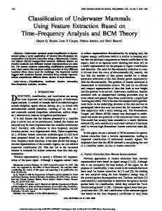
International Journal of Computer Applications (0975 – 8887) Volume 35– No.3, December 2011 of connected components(C) and holes (H): E=C-H … (2.1) It is an important topological descriptor. This simple topological feature as said before is invariant to translation, rotation and scaling. For example the object in the Fig 1 has the Euler number 0 as it has one connected component and one hole.
Fig 2: Boundary Descriptor
2.4 Curvature
Fig 1: Euler number defined by number of connected components This feature does not contribute to classification but it can be used for object filtering. A cell should not have holes in it, since it should be one single connected component. But if it contains one, it means that the image of the cell is corrupted and should be filtered out. This feature can be used for that purpose.
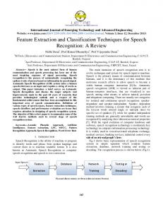
2.3 Boundary Descriptors There are many features that depend on boundary descriptors of objects such as bending energy, curvature etc. For an irregularly shaped object, the boundary descriptor is a better representation although it is not directly used for shape descriptors like centered, orientation, area etc. For boundary descriptor either 4 or 8 connected chain code is used to represent the boundary of an object by a connected componenet24. It starts with a beginning location and a list of numbers representing directions such as d1,d2,d3…..dN. Each direction provides a compact representation of all the information in a boundary. The directions also represent the slope of the boundary. In Figure 2.2, an 8 connectivity chain code is displayed where the boundary description for the boxes with red arrows will be 2-1-0-7-7-0-1-1.
The rate of change of a slope is called the curvature. As the digital boundary is generally jagged, getting a true measure of curvature is difficult. The curvature at a single point in the boundary can be defined by its adjacent line segments. The difference between slopes of two adjacent (straight) line segments is a good measure of the curvature at that point of intersection24. The curvature of the boundary at (xi,yi) can be estimated from the change in the slope and is given by curvature (κ).
κ
=
y yik 1 y i k y i tan 1 i tan xi k xi xi xi k
…(2.2) Curvature (κ) is a local attribute of a shape. The object boundary is traversed clockwise for finding the curvature. A vertex point is in a convex segment when the change of slope at that point is positive; otherwise that point is in a concave segment if there is a negative change in slope as shown in Fig 3.
Fig 3: Curvature of a boundary
2.5 Bending Energy The descriptor called bending energy is obtained by integrating 30
International Journal of Computer Applications (0975 – 8887) Volume 35– No.3, December 2011 the squared curvature through the boundary length. It s a robust shape descriptor and can be used for matching shapes.
1 Eo L 2 R
L
( )
2
p 1
Eo
2.8 Histogram Based Features Histogram of an image is the distribution of any intensity levels in the range24. Histogram of an image has information of general properties of the image. Let u be a random variable representing a gray level in a given region of image.
Pu ( x) … (2.3)
The value 2 / R will be obtained as its minimum for a perfect circle with radius and the value will be higher for an irregular object.
number of pixels with gray level x Total number of pixel in the region
x 0, L 1
… (2.6) Common features derived from histogram are:
2.6 Total Absolute Curvature Total absolute curvature is the curvatures added along the boundary points and divided by the boundary length.
total
1 L
L 1
mi x i pu ( x),
Momemts :
i 1, 2,...
x 0
L
| ( ) |
… (2.7)
p 1
2 total
i
L 1
m i x pu ( x)
Absolute moments:
x 0
... (2.4)
As the convex object will have the minimum value, a rough object will have a higher value.
… (2.8) L 1
Central moments :
2.7 Radial Distance Measures Radial distance is the distance from the center of mass to the perimeter point (xi, yi) as shown in Fig 4. So the radial distance is defined as:
d (i) [ x(i) x ] [ y(i) y ] 2
2
x 0
… (2.9)
Absolute Central moments :
i
L 1
i x mi pu ( x) x 0
… (2.10)
...(2.5) Here d(i) is a vector obtained by the distance measure of the boundary pixels. A normalized vector r(i) is obtained by dividing d(i) by the maximum value of d(i) . The vector r(i) is used for calculating entropy and Fourier descriptor.
i ( x m1 ) i pu ( x)
Entropy :
H E log 2 pu L 1
pu ( x) log 2 pu ( x) x 0
… (2.11)
2.9 Co-occurrence Matrix
Fig 4: Radial Distance
Images of many surfaces can be considered as stochastic textures. In early eighties, the algorithms were mainly based on first and second order statistics of the image pixel gray level values as Spatial domain gray level co-occurrence matrix (SDCM) and Neighboring gray level dependence matrix (NGLDM) . In order to capture the spatial dependence of graylevel values, which contribute to the perception of texture, a two-dimensional dependence matrix known as gray level Cooccurrence matrix is used. This method is based on the spatial distribution and dependence among the gray-levels in a local area of the image. Gray-level Co-occurrence matrix is the two dimensional matrix of joint probability Pd[i,j] defined by first specifying a displacement vector d = [dx, dy], counting all pair of pixels separated by d having gray levels i and j and then normalizing by dividing by total number of pixels. This 31
International Journal of Computer Applications (0975 – 8887) Volume 35– No.3, December 2011 configuration varies rapidly with distance in the fine textures, slowly in coarse textures. Seven texture features extracted from the Co-occurrence matrices are Energy, Contrast, Entropy, Inverse difference moments, Homogeneity, Maximum probability and the Correlation. Entropy measures the randomness of gray level distribution
C1 p d2 i, j
Energy:
i, j
…(2.12)
Information measure (C3 H x , y ) C9 max( H x , H y )
of
Correlation: …(2.20)
M x i * p d (i, j )
Where
i, j
M y j * p d (i, j ) i, j
Contrast: C 2 i j p d2 (i, j )
n
S x (i ) p d (i, j )
i, j
…(2.13)
j 0
n
S y ( j ) p d (i, j )
Entropy: C3 pd i, j log pd i, j …(2.14) Inverse
difference p 2 i, j C 4 i j d |i j| i j …(2.15)
Local homogeneity:
C5 i j i
j
i 0
H x, y pd (i, j ) log( S x (i)S y ( j )) moment:
H x S x (i) log S x (i)
H y S y ( j ) log S y ( j )
2.10 Fourier Transform The Fourier Transform is an important image-processing tool that only characterizes the spatial frequency distribution, but does not consider the information in the spatial domain. The
p d i, j 1 | i j |
discrete Fourier transform of digitized image of size defined by
…(2.16) Maximum probability: C6 max p d (i, j ) i, j
F u, v K
N*N
is
N N
F k, l e jkue jlv k 1 l 1
…(2.17)
Cluster shade: C7 i(i M x j M y ) 3 p d (i, j ) i, j
… (2.21) Where u and v are discrete spatial frequencies. The set of features based on the power spectrum consists of four statistical measures. If F (u, v) is the matrix containing the amplitudes of spectrum and N is the number of frequency components then these measures are given by
…(2.18)
Maximum magnitude:
Cluster prominence: C8 i(i M x j M y ) 4 p d (i, j )
…(1.22) Average Magnitude (Am):
max F (u, v ) (u, v )
i, j
…(2.19)
| F ( u, v ) | u ,v
N
…(2.23) Energy of magnitude:
32
International Journal of Computer Applications (0975 – 8887) Volume 35– No.3, December 2011
| F u, v |2
ln 2
y
u ,v
…(1.24) Variance of Magnitude:
| F u, v A
m
…(2.29) Center frequencies of channel filters must be close to the characteristic texture frequencies or else the filter responses will be poor. Six parameters that must be set when implementing Gabor filter are: F, Q, x, y, BF and B. The frequency (F) and orientation () define center location of the filter. The sets of features based on power spectrum are Moment based on spatialfrequency plane, Rectification, Magnitude response, Local variance of filter response, Syntactic Characterization, Consistent local filter response.
|2
u ,v
…(2.25)
2.11 Gabor Filters As early as 1946, Gabor has found that Fourier analysis is lacking to localize signals in the time domain. He applied Gaussian function as a “window” to improve the Fourier transform. It is referred to as Gabor transform and is applied to analyze the transient signals. Thereafter, Gabor transform led to the general window Fourier transform by the replacement of Gaussian function with other localized window function. In the recent past, Gabor filters, are well recognized as a joint spatial/spatial-frequency representation for analyzing textured images containing highly specific frequency and orientation characteristics. Daugman showed that Gabor filters have optimal joint localization in both spatial and the spatial-frequency domains. Compared to the Fourier transform that only characterize the spatial-frequency in a global approach, the Gabor transform indicates the frequency content in localized regions in the spatial domain so that local deviations embedded in a homogeneous pattern can be distinctly identified. In addition, multi-channel Gabor filtering mimics the visual process in the early stage of the human visual system. By theoretical impact of the works of Daubechies, who has provided the discretization of the wavelet transform (WT), and Mallat, who has established the connection between the WT and the multi-resolution theory, signal processing methods based on Gabor transform and the WT has replaced the Co-occurrence matrix.
-Moment based on spatial-frequency plane: Bigun and Du Buf use moments of the power spectrum of response. - Rectification: Summing the absolute value of the real and imaginary response can also be used to process the complex filter outputs. - Magnitude response: Texture identification can be performed based on the magnitude of the output of the Gabor function. - Local variance of filter response: A complex texture will have fluctuating dominant Gabor filter response. So the local spatial variance of a certain filter response can be calculated to determine the degree to which the filter response is changing. - Syntactic characterization: If all the filter outputs are ranked in order of magnitude, and assigning each filter its own symbol, a syntactic string is created that can be recognized. Ranking is consistent for some texture. - Consistent local filter response: By applying multiple Gabor filters by incrementally increasing the spatial bandwidth (keeping F and constant) if the response is consistent, then texture is regular. The slope of the responses can also be used as a texture feature. Lesser the slope, the more consistent the filter response, results the more regular texture.
A complex Gabor filter represented as a 2 –D impulse response is.
2.12 Markov Random Field
1 x2 1 y 2 h x, y exp 2 2 exp j 2Fx 2 x y y 2 x …(2.26)
The spatial property can be modeled through different aspects, among which, the contextual constraint is a general and powerful one. Markov random field (MRF) theory provides a convenient and consistent way to model context-dependent entities such as image pixels and correlated features. This is achieved by characterizing mutual influences among such entities using conditional MRF distributions. In an MRF, the
The corresponding representation in the spatial frequency domain is
hu, v exp 2 2 (u F ) 2 x2 v 2 y2 …(2.27) x and y are determined by setting the frequency cut off and angular direction
x
2 F tan( B / 2)
2F 2
1
ln 2 2 BF 1
…(1.28)
BF
S are related to one another via a neighborhood system, N N i , i S Ni which is defined as , where is the set of sites in
sites neighboring i,
i Ni
and
field X said to be an MRF on system
i N j j N i
. A random
S with respect to a neighborhood
N if and only if Px 0, x X
P( xi | x S i ) P( xi | xN i ) …(2.30) Note that the neighborhood system can be multi-dimensional. 33
International Journal of Computer Applications (0975 – 8887) Volume 35– No.3, December 2011 Cohen et. al. method is based on modeling textile fabric images through Markov random field (MRF) and use of easily computable statistics as features in place of model parameters during the classification of samples as objective or non objective via a generalized likelihood test.
2.13 Wavelet Transform Many multi-resolution approaches to image classification reflect the effort to combine global and local information. One straight forward approach is to design classifiers based on features extracted from several resolutions, Images at multiple resolutions are usually obtained by wavelet transform,. With the original image being the highest resolution, low resolutions are simply the low frequency bands of wavelet transforms. The wavelet transform was borne out of a need for further developments from Fourier transforms. Wavelets transform signals in the time domain to a joint time-frequency domain. The main weakness that was found in Fourier transform was their lack of localized support, which makes them susceptible to Heisenberg’s Uncertainty principle. The discrete wavelet transforms can in general lead to better image modeling, as for instance to better encoding (wavelet image compression, is one of the best compression methodologies) and to better texture modeling. Also, in this way, we can better exploit the known local information extraction properties of wavelet signal decomposition as well as the known features of wavelet denoising procedures. The emergence of the 2-D wavelet transform as a popular tool in image processing offers the ability of robust feature extraction in images containing objects. Lee et. al have used neural networks to classify objects through energy and entropy features computed from the adaptive wavelet packet expansion of the steel images. De Wouwer conjectures that the texture can be characterized by the statistic of the wavelet detail coefficients and therefore introduce two feature sets: The wavelet histogram signatures, which capture all first-order statistics using a model based approach The wavelet co-occurrence signatures, which reflect the coefficients second-order statistics
3. CLASSIFICATION OF OBJECTS Classification techniques may be categorized in terms of two criteria. Firstly, they can be classified as supervised and unsupervised depending on the involvement of a training dataset. Supervised classification techniques require training data to be defined by the analyst in order to determine the characteristics of each category. The image is, thus, assigned to one of the categories using the extracted discriminating information. Problems of diagnosis, pattern recognition, identification, assignment and allocation are essentially supervised classification problems since in each case the aim is to classify object into one of a pre-specified set of classes. Unsupervised classification, on the other hand, searches for natural groups, called clusters, of objects present within the data by means of assessing the positions of the objects in the feature space. They are automated procedures and therefore require minimal user interaction. Another distinction among classification methods can be made by considering the underlying philosophy and assumptions of the techniques. By this, they can be classified into two groups: statistical
classification and non-statistical classification. Statistical classification procedures employ purely statistical estimations to derive some rules from the data, which leads to some assumptions. The most common assumption of this kind is that the frequency distribution of the data is in Gaussian (or normal) form. However, non-statistical methods do not make any assumptions about the frequency distribution of the data used, and do not use the statistical estimates. The minimum distance and maximum likelihood classifiers can be given as examples of statistical classification methods, whilst the Artificial Neural Network approach, Support Vector Mechanics and knowledgebased methods can be given as examples to non-statistical classification methods.
3.1 Unsupervised Classification In some cases, information concerning the characteristics of individual classes is not available. In such circumstances, an unsupervised classification technique is used to identify a number of distinct or separable categories. In other words, an unsupervised method is used to determine the number of separable groups or clusters in an image for which there is no a priori or insufficient ground truth information available. Such unsupervised methods can be viewed as techniques of identifying natural groups, or structures, within data. While applying an unsupervised method, the analyst generally specifies only the number of groups to be discriminated, and the method generates the specified number of clusters, in feature space [6], that correspond to separable features. Determination of the clusters is performed by estimating the distances between the data in feature space. Unsupervised classification techniques generally require user interaction in specifying the number of groups to be recognized and in labeling the correctly identified areas with the individual feature (or class) label. Owing to the minimal amount of user involvement, they are usually considered as automated procedures. In addition, the assumption, forming the basis of the unsupervised approach, that the object belonging to a particular class will have similar features in feature space, and all classes are relatively distinct from each other in feature space is difficult to satisfy in practice. Consequently, the accuracy of the results obtained by unsupervised classification methods is limited. Hannu Kauppinen et. al. proposes a non-segmenting object detection technique combined with a self organizing map (SOM) based classifier and user interface. The purpose is to avoid the problems with adaptive detection techniques, and to provide an intuitive user interface for classification, helping in training material collection and labeling, and with a possibility of easily adjusting the class boundaries.
3.2 Supervised Classification Supervised classification may be defined as the process of identifying unknown objects by using the information derived from the training data provided by the analyst. The result of the identification is the assignment of unknown object to predefined categories. The main difference between unsupervised and supervised classification approaches is that supervised classification requires training data as input. The training data is used to extract the properties of each individual class within the training data. Supervised classification methods may be grouped into two general categories: statistical and non-statistical algorithms 34
International Journal of Computer Applications (0975 – 8887) Volume 35– No.3, December 2011 (Neural Network, Support Vector Mechanics). In the statistical supervised approach, the information required from the training data varies from one algorithm to another. For example, the maximum likelihood classifier requires the mean vector and variance-covariance matrix for each class. In contrast, supervised non-statistical models do not use any statistical information to identify unknown objects present in an image. Instead, they use all the training data available. This is the principal feature that makes supervised non-statistical models more powerful than their statistical counterparts. As a result, no assumption is made about the frequency distribution of the data in supervised non-statistical models. However, the effect of any incorrect definition of training is more considerable in these models than in the statistical models. This is due to the fact that supervised non-statistical models take every individual training data into consideration, whereas statistical models use only the overall properties of the data. For example, in the estimation of the mean, the effect of misidentified data is smoothed by averaging.
4. CONCLUSIONS
As mentioned earlier, supervised classification is performed in two stages (a) training and (b) classification. In the training stage, the analyst defines the regions that will be used to extract training data, from which statistical estimates of the data properties are computed. In the classification stage, every unknown feature in the test image is labeled in terms of its similarity to specified features. If object is not similar to any of the classes, then it can be allocated to an “unknown” class. The characteristics of the training data selected by the analyst are of considerable importance for the reliability and the performance of a supervised classification process. The training data must be defined by the analyst in such a way that they accurately represent the characteristics of each individual feature used in the analysis.
5. REFERENCES
Two features [7,8] of the training data are of key importance. These are the representativeness (or objectiveness) and the size of the training data. In order to have a representative set of data, the sample selection must be performed by considering the different objects of various sizes at various positions and at various orientation of the object that correctly represent the diversity of each class, so that variations of object position and rotation are considered. The size of the training dataset is also very important if statistical estimates are to be reasonable. Sample size is mainly related to the number of features whose statistical properties are to be estimated. Although supervised classification methods require more user interaction, especially in the collection of training data, they generally give more accurate results compared to unsupervised classification techniques. Therefore, researchers mostly favor them. A new mathematical model that has emerged recently, and which has made a great impact in the scientific community is the artificial neural networks (ANNs) [9, 10]. ANN has attracted increasing attention from researchers in many fields during the last decade, resulting in studies aiming to solve a wide range of problems. ANN has been proved to be more robust compared to conventional statistical classifiers in recognizing patterns from noisy and complex data and in estimating their nonlinear relationships. In short, it is known to be good at learning the internal representation of data in any form.
Feature extraction is the process to reduce the dimensionality of the data, while Classification can be viewed as the process of converting raw data to categorized meaningful information. Number of approaches for feature extraction such as simple geometric descriptors, Topological descriptors, Boundary descriptors, Histogram based methods, Co-occurrence matrices, Fourier transform, Gabor filter, Markov random field, Wavelet transform, CSS descriptors, Grid descriptors n-tuple methods are discussed. The feature based technique is used for feature extraction of the signature images for this research work due to its simplicity and ease of operation. This technique can be efficiently run on a parallel processing system due to the unconnected nature of the attributes for real world problems. The concept of classification is also discussed in this chapter. It has been found that the classification of objects can be achieved by use of representative datasets and employing more powerful classification techniques. Artificial neural network is chosen as it is non parametric in nature. [1] Peng, H.C., Long, F., and Ding, C., Feature selection based on mutual information: criteria of max-dependency, maxrelevance, and min-redundancy, IEEE Transactions on Pattern Analysis and Machine Intelligence, Vol. 27, No. 8, pp. 1226–1238, 2005. [2] Nguyen, H., Franke, K., Petrovic, S. (2010) "Towards a Generic Feature-Selection Measure for Intrusion Detection", In Proc.International Conference on Pattern Recognition (ICPR), Istanbul, Turkey. [3] M. Hall 1999, Correlation-based Feature Selection for Machine Learning [4] Hai Nguyen, Katrin Franke, and Slobodan Petrovic, Optimizing a class of feature selection measures, Proceedings of the NIPS 2009 Workshop on Discrete Optimization in Machin Learning: Submodularity, Sparsity & Polyhedra (DISCML), Vancouver, Canada, December 2009. [5] Muhammed H. Hamid, “What is FeatureVector Based Analysis” Swedish Society for Automated Image Analysis Symposium, 2001, pp 14 – 15. [6] Guyon Isabelle, Elisseeff André, “An Introduction to Variable and Feature Selection” 2003, pp 1157-1182. [7] Hervé Stoppiglia, Gérard Dreyfus, Rémi Dubois, Yacine Oussar, “Ranking a Random Feature for Variable and Feature Selection” 2003, pp 1399- 1414. [8] Armand S, Blumenstein M, Muthukkumarasamy V, “Offline Signature Verification using the Enhanced Modified Direction Feature and Neural-based Classification” International Joint Conference on Neural Networks, IJCNN, Vol 06, 2006,pp 684 – 691. [9] Blumenstein M, Liu X.Y, Verma B, “A modified direction feature for cursive character recognition” International Joint Conference on Neural Networks, IEEE Proceedings. 2004, Vol 4, pp 2983 – 2987 [10] Paola, J. D. and Schowengerdt, R. A., “Comparisons of neural networks to standard techniques for image classification and correlation,” Proceedings of the International Geo-science and Remote Sensing Symposium (IGARSS’94), 1404-1406, Pasadena, USA, 1994
35