results demonstrate the effectiveness of the two methods as compared to other
photo-consistency based disparity estimation techniques. 1 Introduction. A light ...
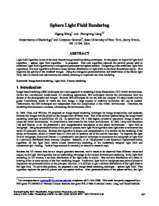
PHOTO-CONSISTENCY AND MULTIRESOLUTION METHODS FOR LIGHT FIELD DISPARITY ESTIMATION Adam Bowen, Andrew Mullins, Nasir Rajpoot, Roland Wilson University of Warwick, United Kingdom {fade, andy, nasir, rgw}@dcs.warwick.ac.uk Keywords: image based rendering, disparity estimation, light field rendering
Abstract
Light fields can be used to generate photorealistic renderings of a scene from novel viewpoints without need for a model of the scene. Reconstruction of a novel view, however, often leads to ghosting artefacts, which can be relieved by correcting for the depth of objects within the scene using disparity compensation. Disparity estimation offers a solution to both better reconstruction and compression of large amounts of data in light fields. In this paper, we present two novel methods of disparity estimation for light fields: a global method based on the idea of photo-consistency and a local method which employs wavelet subbands for initial disparity estimation and Kalman filtering to refine the estimates. Experimental results demonstrate the effectiveness of the two methods as compared to other photo-consistency based disparity estimation techniques.
1 Introduction
A light field [9, 6] captures a large array of images of a scene in a representation that allows fast reconstruction and preserves view dependent effects. Unfortunately, they also require a large number of source images making them prohibitive for the use in video sequences. We present techniques for disparity estimation over light fields that can be used to reduce the number of source images required to reconstruct novel viewpoints and also compress the source data. When reconstructing a novel view of a light field scene, one way in which we may attempt to relieve ghosting artefacts is to estimate, and correct for, the depths of objects within that scene. This is the aim of disparity estimation and compensation which is a well studied field within the context of stereo pairs. When performing disparity estimation, we attempt to obtain a set of correspondences between the pixels from one view of a scene, and the pixels of a different view of the same scene. Local disparity estimation computes the correspondences between each pair of adjacent cameras in a light field array. As the cameras are closely spaced, the problems that occlusions bring to the estimation of depth are limited to small areas around depth discontinuities.
Global techniques are more sensitive to these occlusions. We apply a photo-consistent approach, commonly used in reconstruction, to estimate disparity for the source images using both existing and novel metrics. The results of this technique are compared to our multiresolution wavelet approach for local disparity estimation.
2 The Photo-Consistency Approach
Photo-consistency is a global method for estimating the depth variation in a scene. Essentially, each potential depth is considered by projecting the point into every camera view and comparing the pixel colours with a photo-consistency metric. It is commonly used in space carving algorithms [3, 4, 8, 10] to create a model of the object that can be used to reconstruct novel viewpoints. It can also be used in a more direct manner [5] to reconstruct from the novel viewpoint itself. Taking the desired viewpoint into account has the advantage of allowing the photo-consistency of a reconstruction colour to be computed rather than the photo-consistency of a reconstructed depth. Photo-consistency is a global method in that it considers every source camera when examining potential depth values, it does not consider local information within each image. We present a photo-consistency approach for disparity estimation and compare it with our more local multi-resolution approach. The most significant problem with using photo-consistency as a reconstruction technique is the computation time of most photo-consistency algorithms. This makes it difficult to reconstruct in real time or apply it to video sequences. With disparity estimates we can apply warping techniques [7, 11] to reconstruct novel viewpoints significantly faster without encountering many of the aliasing artefacts found in normal light fields.
2.1 Existing Metrics
We have n images, I1 to In . Ii (x, y) denotes the colour of the pixel (x, y) in the ith image. For convenience we shall also define Ii (v) to be the projection of a point v in some common basis into the ith image. If Pi is a homogenous 3 × 4 projection
matrix for the ith camera then Ii (v) = Ii (π(Pi v))
(1)
π(x, y, w) = (x/w, y/w)
(2)
For a virtual viewpoint V , we shall also define oV to be the position of the reconstruction camera and rV (x, y) to be the ray emanating from pixel (x, y) in the reconstruction camera’s image plane. For a pixel (x, y) and depth z, the corresponding point in the common basis is then XV (x, y, z) = oV + zrV (x, y)
(3)
Some metrics also use the ray vectors from the source data cameras. Let ri (x, y) be the ray emanating from pixel (x, y) in the ith camera’s image plane. For notational convenience, we shall also define ri over the common basis ri (v) = ri (π(Pi v))
n Y
e−βρ(kIi (XV (x,y,z))−C(x,y)k)
(5)
i=1
where C(x, y) is the reconstruction colour for pixel (x, y). We set C(x, y) to be the mean colour at each depth z Pn Ii (XV (x, y, z)) C(x, y) = i=1 (6) n where β is a positive real constant, and ρ is a robust kernel, we achieve best results with the absolute distance ρ(x) = |x|. In the cases where XV (x, y, z) projects to a pixel outside the image we set ρ(x) to be the maximum distance. This requirement means that the photo-consistency of pixels that cannot be seen by all cameras is significantly reduced. The metric also relies on the choice of C(x, y). With no prior information, and without searching colour space (as Fitzgibbon et al do) it is difficult to select this colour correctly. Isodoro and Sclaroff [8] proposed a weighted metric that compares every pair of pixels to one another, and so does not need to select this colour C(x, y). For clarity we drop the (x, y) in the following equations and consider only a single pixel. pV (z) = e
−qV (z)
(7)
where qV (z) =
Pn
i=1
Pn
j=1,j6=i wi,j (z)d(Ii (XV (z)), Ij (XV Pn Pn i=1 j=1,j6=i wi,j (z)
d(c1 , c2 ) =
max
l∈{R,G,B}
|(c1 − c2 )l |
(10)
With this metric, we only compare samples when XV (z) projects to a pixel in both cameras i and j, so if it projects outside the image plane we set wi,j and wj,i to zero. This means that the range of depths searched must be constrained to avoid a point projecting to too few cameras to provide a good result. Because this metric is designed for use in space carving algorithms, it also takes no account of the reconstruction viewpoint. 2.2 Novel Representative Metric
(4)
Fitzgibbon et al [5] describe the traditional photo-consistency p of the pixel (x, y) at depth z as pV (x, y, z) =
which is simply the dot product of the two rays clamped between 0 and 1. The distance between two colours d(c1 , c2 ) is simply the largest error across all three colour channels
We introduce a novel metric designed to tackle the problems with the two aforementioned metrics. We wish to construct a metric that uses all the available information to choose the best reconstruction colour and depth for a given reconstruction viewpoint. The traditional metric assumes all the cameras provide equally accurate information. In a scene with view dependent lighting or occlusions, this is often not the case. Equally, Isodoro and Sclaroff’s weighted metric does not use the reconstruction viewpoint. Neither metric explicitly deals with the case where some elements of the scene may not be visible to all cameras. We can say that at least one camera must provide a relatively accurate sample of the colour of the pixel we wish to reconstruct. We select this sample by minimising a distance function over the set of reprojected pixels. We can also say that those cameras closest to our reconstruction viewpoint will provide the best estimate of the pixel we are reconstructing. Since view dependent lighting conditions often vary with the cosine (or a power of the cosine) of the angle, a good weighting scheme to apply is the dot product of the actual pixel ray and the ray emanating from the camera. Finally, we use the same distance measure as Isodoro and Sclaroff because it is fast to compute and more robust than squared difference methods. For clarity, we consider a single pixel. pV (z) = e−βqV (z) where qV (z) =
(z)))
(11)
min
i=1,2,...,n
( Pn
j=1,j6=i
wj (z)d(Ii (XV (z)), Ij (XV (z))) Pn j=1,j6=i wj (z) (12)
(8)
where our weighting function, wj is now defined as
wi,j (z) is the weight of the distance between cameras i and j, defined as follows
wj (z) = [clamp(0, rj (XV (z)).rV , 1)] ,
wi,j (z) = clamp(0, ri (XV (z)).rj (XV (z)), 1)
(9)
k
(13)
ri , rV and d(c1 , c2 ) are defined as before, β and k are constants. The constant k varies depending on how much
)
occlusion and view dependent lighting is present in the scene. We found that a value of around 2 for k yields best results for diffuse scenes. As with Isodoro and Sclaroff’s method, we set wi to zero when XV (z) projects to a point outside the camera’s image plane. However, we also apply the constraint that at least m cameras must be able to see the point, otherwise the photo-consistency is set to zero. This prevents points that can be seen by only one or two cameras from dominating the photo-consistency measure. Setting m to around one-third of the available cameras (m = n/3) works well with our camera arrangement. We shall refer to this metric as a weighted representative metric.
3 Multiresolution Disparity Estimation
search window (of ± 8 pixels) is either purely horizontal, or purely vertical depending on relative positions of the two cameras. The input to our algorithm is the 2D discrete wavelet transform (DWT) of both images. In testing, the Haar wavelet transform outperformed all other wavelets and so is our wavelet of choice. Typically, the DWT is performed to 5 levels. The low pass band is ignored and disparity estimation begins on the appropriate lowest resolution high pass image. Following estimation of disparity in the lowest resolution high pass band we use the disparity values to guide our search window at the next finest resolution. By using a constant block size and search window at every scale our estimates become more refined as we progress up the wavelet tree (Figure 2).
Our proposed local disparity estimation between views is performed on the wavelet coefficients of each image. The wavelet representation of an image is multi-resolution, allowing us to apply efficient multi-resolution disparity estimation algorithms which have been well studied within the context of stereo pairs, e.g. [2]. In addition, the efficient computation of the wavelet representation is ideal for large volumes of light field data [13]. Despite its advantages, problems associated with estimating scene change using fully decimated wavelet coefficients are well known. Firstly, the wavelet representation is highly shift variant [1]. Thus, small translations between two input images could produce large differences in the wavelet coefficients (Figure 1). Secondly, we are presented with three bands of coefficients at each resolution: a horizontal high pass image, a vertical high pass image, and a horizontal and vertical high pass image. Unless we have prior knowledge about the direction of disparity or motion, we do not know on which set of coefficients to perform our estimation at that level. Fortunately, light field data typically consists of an array of images, arranged on a regular grid [9]. We may assume in this case that disparity between two adjacent cameras is purely vertical or purely horizontal. As a result, the choice of subband in which to perform disparity estimation appears obvious: select the detail image containing horizontal energy when estimating disparity between two horizontally separated images, and select the detail image containing vertical energy when estimating disparity between vertically separated images. In addition, the uncertainty caused by the shift invariance of the wavelet representation is reduced because we have such a strong prior on the likely direction of disparity. To estimate disparity using the coefficients of the DWT, our proposed algorithm begins by selecting the appropriate subband at the lowest resolution in each image. A simple blockbased search is performed using 8 × 8 blocks with a 4 pixel overlap. We search for the most similar block in the target image using normalised cross correlation as our measure. The
Figure 2: Propagation of disparity estimates between multiple resolutions of wavelet subbands 3.1 Kalman Filtering In addition to the simple multiresolution refinement of disparity estimation, we may use Kalman filter [12] to the results across scales. The state for an original pair of images i, j of size m, n is si,j = (δ(x1 , y1 ), δ(x2 , y1 ), ..., δ(xn , ym )) to be estimated is a disparity value for each pixel at full resolution (with corresponding covariance matrix P ). At each resolution k, we form a prediction of the state and covariance according to the Kalman predict equations: s− k = Ask−1 Pk−
T
= APk−1 A + Q
(14) (15)
where A = I is the process matrix which in this case is static. The estimates at each resolution, appropriately scaled and interpolated to full resolution, are our measurements z which are computed using the method outlined above. Note, because of this scaling we add some process noise Q = αI to flatten our distribution to reflect the fact that our estimates will become more accurate as we process the higher resolutions. We take our measurement noise R to be a function of the cross correlation peak for each correspondence. Since z is a direct
6 2.5
2
5 1.5
1
4
0.5
3
0
−0.5
2 −1
−1.5
1 −2
0
1
2
3
4
5
6
7
−2.5
1
1.5
2
2.5
3
3.5
4
Figure 1: The shift variance of the discrete wavelet transform in 1D. An input signal is shown (left), along with the resulting high pass coefficients of the original input signal, and those of the input signal shifted by 1 place (right). depth maps were then used to compute horizontal and vertical disparity maps for each camera by re-projection. If the depth for pixel (x, y) from viewpoint V is zV (x, y)
function[s,P] = DISPARITY(img1,img2) dwt1 ← DWT(img1); dwt2 ← DWT(img2);
zV (x, y) = argmax pV (x, y, d)
(19)
d
for i ← level to 1 s ← A * s;
then the disparity map δi,j (x, y) between image i and image j is computed as
P ← A * P * TRANSPOSE(A) + Q; [z,R] ← NORMALISED CROSSCORR(BAND(dwt1,HL,i),BAND(dwt2,HL,i),s); z ← POWER(2,i) * INTERP(z,POWER(2,i));
δi,j (x, y) = π(Pj XV (x, y, zV (x, y))) − (x, y)
(20)
noting that the virtual viewpoint V is equivalent to camera i. Disparity maps were also computed using the multiresolution algorithm described in Section 3. Because we have a geometric model for our light field, we can compare these estimates with the perfect disparity maps. Figure 4 shows images from our two light field data sets.
R ← INTERPOLATE(r,POWER(2,i)); K ← P * H * 1 / (H * P * TRANSPOSE(H) + R); s ← s + K * (z - H * s); P ← (I - K * H) * P; end;
Figure 3: Pseudo code for multiresolution disparity estimation.
4.1 Teddy Results
measurement of the state s, the relationship between them is simply the identity matrix H = I. Hence, we update our estimates using the Kalman filter update equations as follows:
Figure 5(a) shows the peak signal to noise ratio (PSNR) of the disparity maps computed for each image in the light field using the traditional photo-consistency metric. The average PSNR is 24.5dB. Figure 5(b) shows where the errors occur in the estimation of a single disparity map. Generally the body of the teddy is correctly identified except where occlusions are present (notably around where the legs join the body) but the background is generally not well identified. This is due to the significant amount of occlusion of the background by teddy and also the fact that not all cameras can see the edges of the background.
Kk = Pk− H T (HPk− H T + R)−1
(16)
+ Kk (zk − Hs− k) Pk = (I − Kk H)Pk−
(17) (18)
sk =
s− k
Figure 3 shows the pseudo code for our final disparity estimation algorithm.
4 Experimental Results
We used the photo-consistency metrics described in Section 2 to compute depth maps for every image in a synthetic lightfield comprised of an 8×8 camera plane and a 256×256 image plane. The depth at each pixel was determined by finding the depth value that maximised the photo-consistency metric. The
Figure 6(a) shows the PSNR of the disparity maps computed for each image in the light field using Isodoro and Sclaroff’s weighted photo-consistency metric. The average PSNR using this metric is 5.74dB, mainly because of the large amount of error whilst estimating the background. The significantly higher error rates are due to the volume selected to be searched, a much tighter volume is needed for this metric to perform well. Figure 6(b) shows how the error is distributed over a single
(a) Teddy Light Field
(b) Dragon Light Field
Figure 4: Image (4, 4) from each of our light field data sets
7 25 24.9 6 24.8 24.7
5
v
24.6 4
24.5 24.4
3 24.3 24.2
2
24.1 1
1
2
3
4 u
5
6
7
24
(b) Squared error on the disparity map (4, 4) → (5, 4)
(a) PSNR Across the light field images
Figure 5: Results using the traditional photo-consistency metric for the Teddy light field
7
11
6
10
9
5
v
8 4
7 3 6 2 5 1
1
2
3
4 u
5
6
(a) PSNR Across the light field images
7
(b) Squared error on the disparity map (4, 4) → (5, 4)
Figure 6: Results using Isodoro and Sclaroff’s weighted photo-consistency metric for the Teddy light field
v
7
30
6
29
5
28
27
4
26 3
25 2 24 1
1
2
3
4 u
5
6
7
(a) PSNR Across the light field images
(b) Squared error on the disparity map (4, 4) → (5, 4)
Figure 7: Results using our weighted representative photo-consistency metric for the Teddy light field disparity map. The measure performs well on un-occluded parts of teddy but very poorly on the background. Figure 7(a) shows the peak signal to noise ratio of the disparity maps computed for each image in the light field using our photo-consistency metric. The average PSNR is 26.3dB, an improvement of 1.8dB over the traditional metric. Figure 7(b) shows how this improvement is seen in an individual disparity map. Here the metric has correctly identified the background and body of teddy except where occlusion becomes a significant factor. It is also worth mentioning that the maximum error is greater with this technique than with the traditional metric. The disparity maps estimated using our multiresolution technique significantly improve on those estimated globally in terms of the PSNR when compared to the ideal disparity maps. Figure 8(a) shows the PSNR of each disparity map across the array of cameras. The PSNRs range from 30dB to 35dB, with an average of 32.3dB. The difference image between the ground truth disparity values, and the estimated values for the camera pair (4,4) and (5,4) is shown in Figure 8(b). 4.2 Dragon Results We also generated disparity maps for our far more challenging ’dragon’ light field. The dragon light field uses Stanford’s publicly available dragon model together with a highly specular surface. We computed photo-consistent disparity maps using our metric and the traditional metric. The dragon light field has a uniform background so there is no information to estimate disparity maps. Because inaccurate values in the background generally have little effect on the reconstruction, we compute the PSNR over the shape adapted region only. Because this scene has significantly more view dependent artefacts, we used a value of k = 20 to weight in favour of closely aligned samples and a value of m = n to prevent the
uniform background being identified as photo-consistent. Here our metric significantly outperforms traditional techniques because cameras are weighted in favour of those more closely aligned with the reconstruction ray. The average PSNR with a traditional photo-consistency metric was 24.8dB, and 38.3dB with our weighted representative metric. Figure 9(a) and figure 10(a) contrast how the PSNR varies across the light field whilst Figure 9(b) and Figure 10(b) show how the squared error vary within an individual image. Figures 11(a) and 11(b) show the results using our multiresolution disparity estimation. Again it significantly outperforms the photo-consistency approach producing a mean PSNR of 46.0dB.
5 Conclusions
In this paper, we have compared several common approaches to estimation of disparity with two novel techniques, one based on photo-consistency and one based on local disparity estimation. The results we have obtained on two test data sets demonstrate that the new methods perform significantly better than previous techniques based on photo-consistency. We are currently investigating ways to improve the quality of our results using a local surface model.
Acknowledgements
This research is funded by EPSRC project ’Virtual Eyes’, grant number GR/S97934/01.
7
35 6
34 5
v
33 4
32 3
31 2
1
30 1
2
3
4 u
5
6
7
(b) Squared error on the disparity map (4, 4) → (5, 4)
(a) PSNR Across the light field images
Figure 8: Results using our multiresolution approach for the Teddy light field
7 27 6 26 5
v
25 4 24
3 23
2
1
22
1
2
3
4 u
5
6
7
(b) Squared error on the disparity map (4, 4) → (5, 4)
(a) PSNR Across the light field images
Figure 9: Results using the traditional photo-consistency metric for the Dragon light field
7
44 43
6 42 41 5
v
40 39
4
38 37
3
36 2
35 34
1
1
2
3
4 u
5
6
(a) PSNR Across the light field images
7
(b) Squared error on the disparity map (4, 4) → (5, 4)
Figure 10: Results using our weighted representative photo-consistency metric for the Dragon light field
7 50
6
49
5
48
4
47
3
46
45
2
44 1
1
2
3
4
5
6
7
(a) PSNR Across the light field images
(b) Squared error on the disparity map (4, 4) → (5, 4)
Figure 11: Results using our multiresolution disparity estimation for the Dragon light field References [1] Andrew P. Bradley. Shift-invarience in the discrete wavelet transform. In Digital Image Computing: Techniques and Applications, volume 4, 2003. [2] A. D. Calway, H. Knutsson, and R. Wilson. Multiresolution estimation of 2-d disparity using a frequency domain approach. In British Machine Vision Conference, pages 227–236. springer-verlag, September 1992. [3] German K. M. Cheung, Simon Baker, and Takeo Kanade. Visual hull alignment and refinement across time. In Proceedings of the IEEE Conference on Computer Vision and Pattern Recognition, Madison, Wisconsin, June, 2003, volume II, pages 375–382, June 2003. [4] Peter Eisert, Eckehard Steinbach, and Bernd Girod. Multi-hypothesis, volumetric reconstruction of 3D objects from multiple calibrated camera views. In Proceedings ICASSP ’99, Phoenix, USA, pages 3509– 3512, March 1999. [5] A.W. Fitzgibbon, Y. Wexler, and A. Zisserman. Imagebased rendering using image-based priors. In Ninth IEEE International Conference on Computer Vision, Nice, France, October 2003, volume 2, pages 1176–1183, October 2003. [6] Steven J. Gortler, Radek Grzeszczuk, Richard Szeliski, and Michael F. Cohen. The lumigraph. In Proceedings of ACM Siggraph ’96, New Orleans, LA, August 1996, pages 43–54. ACM Press, New York, August 1996. [7] W. Heidrich, H. Schirmacher, H. K¨uck, and H. P. Seidel. A warping-based refinement of lumigraphs. In Vaclav Skala, editor, Proc. Winter School in Computer Graphics (WSCG) ’99, Plzen, Chech Republic, February 1999, pages 102–109, February 1999. [8] John Isodoro and Stan Sclaroff. Contour generator points for threshold selection and a novel photo-consistency
measure for space carving. Technical Report BUCSTR-2003-025, Boston University Computer Science, December 2003. [9] Marc Levoy and Pat Hanrahan. Light field rendering. In Proceedings of ACM Siggraph ’96, New Orleans, LA, August 1996, pages 31–42. ACM Press, New York, August 1996. [10] Wojciech Matusik. Image-based visual hulls. Master of science in computer science and engineering, Massachusetts Institute of Technology, February 2001. [11] Hartmut Schirmacher. Warping techniques for light fields. In Proc. Grafiktag 2000, Berlin, Germany, September 2000, September 2000. [12] G. Welch and G. Bishop. An introduction to the kalman filter. [13] J. W. Woods and S. D. O’Neil. Subband coding of images. IEEE Transactions on Acoustics, 34(1):1278–1288, 1986.