PHOTOGRAMMETRIC BRIDGING USING FILTERED ... - CiteSeerX

PHOTOGRAMMETRIC BRIDGING USING FILTERED MONOCULAR OPTICAL FLOW J. F. C. Silva a*, R. L. Barbosa b, M. Meneguette Junior a, R. B. A. Gallis a a

Faculty of Science and Technology, Unesp, Brazil - (jfcsilva, messias)@fct.unesp.br b São Paulo Associate Faculty, São Paulo, Brazil - [email protected] Commission ICWG V/1

KEY WORDS: Mobile Mapping, Optical Flow, Monocular Velocity, Image Sequence, Image Orientation

ABSTRACT: Under certain conditions the positioning and orientation sensors such as INS and GPS of a land-based mobile mapping system may fail for a certain time interval. The consequence is that the images captured during this time interval may not be oriented properly or even may have no orientation. This article presents a solution to orient the images based only on image processing and a photogrammetric technique without any external sensors in order to overcome the lack of external orientation. A land-based mobile mapping system with a pair of video cameras and a GPS receiver was used to test the proposed methodology on an urban flat road. The video cameras were mounted on the roof of the vehicle with both optical axes parallel to the main road axis (Y). The methodology is based on the velocity estimation of the vehicle, which is done in two steps. Initially, the dense optical flow is computed then the velocity estimation is obtained through a filtering strategy that consists of using radial vectors in the low parts of the images. These radial vectors are detected by the Canny algorithm. The vehicle velocity is re-estimated after eliminating the optical flow outliers. With the re-estimated velocity and with the video sampling time the spatial displacement of each image (with respect to the previous one of the sequence) is determined. The displacement is used as an approximation to the image position. Homologous points are manually selected in the first stereo pair. Assuming an arbitrary orientation for the first pair, the corresponding object point coordinates are computed by photogrammetric intersection. The orientation is computed by phototriangulation with additional parameters. Following, new bases are included, one by one, and the phototriangulation is computed for every additional basis. The photocoordinates are determined by forward area correlation. This process has been called photogrammetric bridging or traverse. The results show that the estimated velocity is pretty close to the true one and the quality of the least square adjustment is quite acceptable, considering that no external sensors were used.

1. INTRODUCTION The GPS (Global Positioning System) receivers and the INS (Inertial Navigation System) sensors are very important elements of a land-based mobile mapping systems (LBMMS), considering that the position and orientation of such system, which is built in a vehicle, are given by an integrated solution of GPS and INS data (Tao et al., 1999; Tao et al. 2001). In general, a LBMMS has also at least a pair of video cameras mounted on the roof of such vehicle. The camera optical axes are parallel to each other and they point forward so that it is possible to get a sequence of road image stereoscopic pairs as the vehicle moves along roads. The vehicle position and orientation are then extended to these image pairs so that it is possible to map interest objects such as poles, trees, garbage cans, curbs, road center lines, and many other features. Government and private companies have great interest on these data in order to get information for the purpose of planning, control, and maintenance. However, under certain conditions such as in an urban environment with trees and tall buildings the GPS signal may be blocked for a certain time interval. Then INS data are used to complement the vehicle position and orientation. If the time interval lasts a few seconds the INS data may not be useful because they are degraded with the time due to the cumulative internal error process. Additionally, a low cost LBMMS may not have a complete system either without an INS mechanism or with only one GPS antenna. * Corresponding author.

This article presents a solution to orient the image pairs considering that the external sensors are not available. The optical flow is used to estimate the velocity of the vehicle and then the relative positioning among the image pairs considered that the image sequence time interval is known. The relative positioning and a set of homologous points manually extracted in the first stereo pair are used to compute the photogrammetric traverse which means to add and to orient the image pairs consecutively and automatically.

2. OPTICAL FLOW Optical flow is the 2D distribution of the apparent velocity of the intensity pattern movement in the image plane. In other words, the field of optical flow consists of a dense field of velocity where each pixel in the image plane is associated to only one velocity vector. If the time interval between two consecutive images is known the velocity vectors can be converted into displacement vectors and vice-versa (Shi; Sun, 2000). The optical flow – or the image velocity – computation is a fundamental problem in the image sequence processing and can be useful in many tasks such as scene interpretation, exploring navigation, object following, time-to-collision evaluation, object segmentation, video coding, robot vision, and many others (Tekalp, 1995). The methods to compute the optical flow can be classified in three main groups: differential,

correlation, and frequency-energy-based techniques (Beauchemin; Barron, 1995). In the differential techniques, the initial hypothesis for the optical flow computation is that the intensity between different frames of a sequence is approximately constant in a short time interval, which means that the displacement is minimal. The image velocity is computed from the space-time differentials of the image intensity. The image intensity (dominium) is assumed as continuum (or differentiable) in the space and time. This can be written according to the Horn and Schunck (1981) expression:

   I x; t   I x  x , t  t 

(1)

  Where I ( x , t ) is the image intensity function, x  ( x, y ) is

 x is the displacement of  x, t  after the time t . The right side of (1) is

the position vector in the image, and an image region

expanded using Taylor series:

  I  x; t   I .x  tI t  O 2 Where

I  ( I x , I y )

(2)

is the intensity spatial gradient; I t is

the first order term related to the time of

 I ( x, t )

and

O2

are

the second order and higher terms which can be neglected.  I ( x , t ) is subtracted from both sides and the result is divided by

t , then:

  x I .  I t  0  I .v  I t  0 t

(3)

  x y  v  (u , v)   ,   t t 

(4)

 2 V x  xy  f f hf  V 2 v  xy  y f hf

u

(5)

where f is the camera focal length, h is the camera height taken from the floor, ù is the angular velocity and (x,y) are the image plane coordinates. The equations (5) describe the 2D movement when the vehicle travels on a flat road considering a static scene. In other words, they consider that the unique movement comes from the cameras fixed on the top of the vehicle. This kind of movement is called passive navigation (Giachetti et al., 1998) and the authors state that the estimated velocity can be very different from the true one. The angular and translational velocities are computed by the least square method and so the use of the dense optical flow is not recommended either for the computational effort (many points) or the presence of a lot of noises (low quality results). In order to reduce the quantity of vectors used in the translational velocity estimation, the following procedure is advisable: (i) to take the vectors in the region of interest (lower half of the image), (ii) to take only vectors with radial pattern (because of the forward vehicle displacement and the planar image displacement), (iii) and the radial vectors must have their origins in points (pixels) detected by the Canny algorithm (a borderline point or pixel) (Canny, 1986). This filtering technique is equivalent to a first stage which is complemented by a second one which eliminates those residuals that fall out of the interval:

u  su , u  su  and v  sv , v  sv 

Where (4) is the velocity in the image or the optical flow and (3) is the optical flow constraint equation and it defines a unique local restriction on image displacement (Horn; Schunck, 1981; Barron et al., 1994). The accuracy of the differential techniques depends mainly on the estimation of the intensity function partial derivatives. Besides its simplicity, the finite difference method is not able to separate signal (actual data) from noise. In order to eliminate or reduce such drawback, in general the image is smoothed by a Gaussian filter for instance. In the real world, the 2D displacement determination process is complex because both sensor and objects in the scene may be moving relating to each other. Camera vibration, due to irregular surface roads, is another important cause to make difficult the displacement determination based on optical flow. Clouds and shadows affect the scene illumination and this may change the image sequence intensities which bring more difficulties to this estimation process.

3. VELOCITY ESTIMATION Considering that the vehicle translational velocity is parallel to the camera optical axis (Y) the optical flow is given by (Giachetti et al., 1998):

u is the average (eq. 4) and

su

(6)

is the standard deviation of the

residuals for the u component of the optical flow; v and

sv

are

the same related to the v component. The second stage reestimates the velocity based only on those radial vectors that are in the one standard deviation interval (eq. 6).

4. IMAGE ORIENTATION With the velocity estimated from a stereo pair sequence the relative positioning is computed for each camera using the video sampling rate (30 frames per second). Homologous points are manually extracted in the first stereo pair. The related object point coordinates are estimated by photogrammetric intersection using the collinearity equations with additional parameters (x0, y0 and k1):

  x  x0  f  y  y  f 0 

Nx   x  x0 k1 r 2 D Ny   y  y 0 k1 r 2 D

(7)

These object coordinates are used for the photogrammetric resection of the second stereo pair together with the new values for the perspective center coordinates given by the forward displacement which is derived from the estimated velocity and

the video sampling rate. Rotation matrix is approximated by the identity matrix. A forward area correlation determines the photocoordinates in the second pair which is pretty similar to the first one so that the optical flow technique is differential. The correlation window is minimal so the accuracy is improved. This process is repeated for every stereo pair added to the sequence and it is called photogrammetric bridging or traverse, which means a sequential procedure of photogrammetric intersection and resection (Silva et al., 1999; Silva et al., 2000; Silva et al., 2003). Besides the functional model, two types of constraints are considered to compute the spatial resection: stereo basis and velocity constraints. The stereo basis constraint uses the fixed distance between the perspective centers (eq. 8) and the velocity constraint takes the stereo basis advances (given by the basis displacement) divided by the time (eq. 9):

Bi 

X

l C

 X Cr

2

  Y

VX  VY  VZ 

l C

 YCr

2

  Z

l C

 ZCr

2



Figure 1a. Original image

(8)

XCi 1  XCi

t YCi 1 YCi

(9)

t ZCi 1 ZCi t

and i+1 stand for two consecutive bases. When the velocity is considered as a parameter, the collinearity equations can be rewritten in order to estimate the velocity of the perspective centers (Gosh, 1985):

x f

data, and similarly for the second sequence the reference velocity was 19.75 km/h.

r11 X  Xc tVX  r12Z Zc tVz  r13Y Yc tVY  r31 X  Xc tVX  r32Z Zc tVz  r33Y Y c tVY  ( 9)

r  X  Xc tVX  r22Z Zc tVz  r23Y Yc tVY  y f 21 r31 X  Xc tVX  r32Z Zc tVz  r33Y Yc tVY 

tV X , tVY , tVZ

are the displacements between two consecutive bases in terms of the perspective center coordinates.

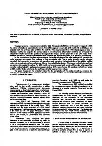
5. RESULTS FROM THE PROPOSED METHODOLOGY Firstly, the results for the velocity estimation are presented. The images were taken on a flat urban road with low illumination at 30 fps. The optical flow was computed and the Canny algorithm was applied to each image to detect the edges. Then each flow was classified according to the procedure advised in section 3. Figure 1a shows the original image and figure 1b shows an example of dense optical flow (5 x 5 needle diagram). Considering the first sequence that corresponds to the first second for both images (left and right) the reference velocity was 19.83 km/h, as computed from the Ashtech Reliance GPS

Figure 1b. Dense optical flow Tables 1 until 4 show the average velocity and the standard deviation (SD) of the two sequences (T: 1 means the 1st second and 2 means the 2nd second) considering the camera at left (L) independently from the camera at the right side (R). Each sequence has 30 images. Table 1 shows the results computed using all the vectors in the region of interest. Table 1. Estimated velocity from all vectors in the regions of interest. AV SD Nr. of SD (km/h) (km/h) vectors (vectors) Cam T Stage 1.57

0.54

230,186

0.00

L

1

1

2.15

0.37

230,186

0.00

R

1

1

1.83

0.76

230,186

0.00

L

2

1

2.07

0.82

230,186

0.00

R

2

1

12.48

7.83

489.59

145.15

L

1

2

9.13

5.19

411.17

129.68

R

1

2

8.02

2.35

697.03

202.56

L

2

2

9.65 3.84 443.72 130.18 R 2 2 As the number of vectors are high (230,186), the velocity estimation has no good quality when compared to the reference values (stage 1). The standard deviation is zero because all vectors of all 30 images of each side were used. In the second stage, the number of vectors was reduced so another velocity value was computed although too low still far from the reference values.

Table 2. Estimated velocity from the regions of interest and with only radial pattern vectors. AV SD Nr. of SD (km/h) (km/h) Vectors (Vectors) Cam T Stage 3.34

0.59

110,367 25972.80

L

1

1

4.07

0.36

107,169 22780.10

R

1

1

3.54

0.57

113,889 27590.10

L

2

1

107,726 24595.40

3.81

0.82

R

2

1

12.39

7.46

485.66

142.82

L

1

2

9.29

5.04

412.90

129.78

R

1

2

8.13

2.18

705.38

210.07

L

2

2

9.91

3.85

447.17

128.70

R

2

2

In the first stage of the second experiment, the velocity was computed with the radial vectors of the regions of interest so a little better value was estimated as compared to the first test. The velocity estimated in the second stage was close to the previous experiment. A possible partial conclusion may be that the second stage acts as filter that separates the radial pattern vectors. The third experiment was done with the vectors which origins lay on points (pixels) detected by the Canny algorithm in the regions of interest no matter the pattern, radial or transversal. Table 3 shows the contribution of those vectors referred to the third experiment. It is evident that the estimated velocities are closer to the reference ones for both stages as compared to the previous experiments. Table 3. Estimated velocity from the regions of Canny. AV SD Nr. of SD (km/h) (km/h) vectors (vectors) Cam 17.72 4.77 1190.55 120.12 L 16.10 3.20 1093.66 77.72 R 12.87 3.64 1694.07 195.19 L 13.08 3.31 1260.41 55.55 R 18.19 4.67 511.52 154.67 L 17.83 3.65 480.07 161.78 R 13.67 4.42 735.52 221.31 L 15.00 3.02 524.62 152.01 R

vectors in the second stage is lesser than that of the first stage so the estimation is even better. This suggests that the remaining vectors are those that actually contain the implicit information related to the vehicle displacement and also that the eliminated vectors are those that really disturbed the estimation process. The average velocity is computed from the left and the right image velocities and it is attributed to all images of the sequence. Then the approximate relative position of every image is computed based on the constant sampling rate (30 fps) or 1/30th of the second. In the first image pair, a set of 17 homologous points was manually measured and the photocoordinates were determined. Together with an arbitrary position and orientation for the first pair, the object coordinates of the 17 points were estimated by least square photogrammetric intersection. A forward correlation between two images at t1 (1st basis) and t2 (2nd basis) for both left and right sequences (figure 2) is computed. pi(t1) is one of the 17 image points determined in the first pair; pi(t2) is the correspondent point in the second pair of the sequence. The position of pi(t2) in the image plane is given by the collinearity equations, the correspondent object coordinates of Pi, and the approximate orientation of the second pair. The perspective center coordinates of the second pair are estimated from the displacement given by the use of the estimated velocity and the 1/30 time interval. The target window is centered at pi(t1) and the search window at pi(t2). The best correspondence indicates the definitive image point pi(t2) that corresponds to pi(t1).

interest and

T 1 1 2 2 1 1 2 2

Stage 1 1 1 1 2 2 2 2

Finally, table 4 presents the results obtained with the procedure proposed in this article. Table 4. Estimated velocity with the proposed methodology. AV SD Nr. of SD (km/h) (km/h) vectors (vectors) Cam T Stage 19.06 3.26 949.17 290.94 L 1 1 18.78 1.95 809.59 263.71 R 1 1 14.53 3.27 1243.86 376.10 L 2 1 14.34 2.83 839.24 252.34 R 2 1 19.67 2.96 510.83 153.35 L 1 2 1.96 482.14 162.35 R 1 2 19.90 3.96 222.83 15.88 735.31 L 2 2 16.51 1.68 520.10 152.77 R 2 2 The filtering methodology reduces the amount of vectors and it improves the velocity estimation in both stages. The amount of

Figure 2. Forward area correlation

This is the technique to determine the image point photocoordinates in the subsequent images. The process is repeated and when a new pair is added to the sequence the adjustment is recomputed. If a ground point does not appear in both images of a new basis it must be excluded. If the degrees of freedom is less or equal to zero a message is sent for the

operator to measure one or more points in the new pair. The figure 3 summarizes the methodology.

Table 6. Adjusted bases and velocities. Bases (m) (m/s) 1 0.93996 2 0.93997 5.48980 3 0.94009 5.49010 4 0.93998 5.48999 5 0.93976 5.49000 6 0.93996 5.48999 7 0.93996 5.48999

6. CONCLUSION The goal of this work was to estimate the positioning and orientation of a road image sequence of stereoscopic pairs without using external sensors or control points. Monocular optical flow was used to compute the velocity and then the displacement between every two consecutive bases. The filtering applied to select only the radial pattern vectors and also those with origins at pixels detected by the Canny algorithm was a strategy that produced a good estimation for the velocity. The basis and the velocity constraints provided improved result as well as the adjustment. In future work it is intended to eliminate the manual measuring of the homologous points in the first basis. The idea is to use a sample of the filtered points. This will represent an attempt to a totally automated methodology.

Figure 3. General methodological work flow

The results that follow were obtained with seven bases (or stereo pairs) which mean fourteen images. The bases were taken every 5/30 s. With all the seven bases the equation system had 476 observation equations, 51 ground coordinates, 7 basis constraints, and 6 velocity constraints. Of course, the adjustment model was composed by the linear(ized) and the constraint equations. The basis constraint used the base length equals to 0.94m and the velocity constraint used the estimated velocity values. Figure 4 shows the sigma zero values accordingly to the experiments.

Barron, J. L., Fleet, D. J., Beauchemin, S. S., 1994. Performance on optical flow techniques. International Journal of Computer Vision, 12(1), pp. 43-77. Beauchemin, S. S., Barron, J. L., 1995. The computation of optical flow. ACM Computing Surveys, 27(3), pp. 433-467. Canny, J., 1986. A computational approach to edge detection. Trans. on Pattern Analysis and Machine Intelligence, v. PAMI8(6), pp. 679-698. Giachetti, A., Campani, M., Torre, V., 1998. The use of optical flow for road navigation. IEEE Transactions on robotics and automation, 14(1), pp. 34-48.

5 4 sigma zero

REFERENCES

3

Gosh, S. K., 1985. Image motion compensation through augmented collinearity equations. Optical Engineering, 23(6), pp. 1014-1017.

2 1 0 1

2

3

4

5

6

7

Horn, B. K. P., Schunck, B. G., 1981. Determining optical flow. Artificial Intelligence, 17, pp. 185-203.

Nr. of stereobases

Figure 4. Number of stereo bases and the sigma zero

Table 6 shows the results related to the adjusted bases and velocity (m/s). The computed velocity does not apply to the first basis.

Shi, Y. Q., Sun, H. 2000. Image and video compression for multimedia engineering: fundamentals, algorithms and standards. CRC Press, Boca Raton, pp. 265-302. Silva, A. R., Batista, J. C., Oliveira, R. A. Camargo, P. O., Silva, J. F. C., 1999. Surveying and Mapping of Urban Streets by Photogrammetric Traverse. In: Proceedings of the International workshop on mobile mapping technology, Bangkok, Thailand, 32(2W10), pp. 5.A.5.1-4.

Silva, J. F. C., Camargo, P. O., Oliveira, R. A., Gallis, R. B. A., Guardia, M. C., Reiss, M. L. L., Silva, R. A. C., 2000. A street map built by a mobile mapping system. In: Proceedings of the XIX International Congress of ISPRS, Amsterdam, Netherlands, Book 2 (Commission II), pp. 506-13. Silva, J. F. C., Camargo, P. O., Gallis, R. B. A., 2003. Development of a low-cost mobile mapping system: a South American experience. Photogrammetric Record, 18(101), pp. 5-26. Tekalp, A. M., 1995. Digital video processing. Prentice Hall, Upper Saddle River, pp. 72-93. Tao, C., Chapman, M. A., El-Sheimy, N., 1999. Towards automated processing of mobile mapping image sequences. In: Proceedings of the International workshop on mobile mapping technology. Bangkok, Thailand. pp. 2-5-1:2-5-10. Tao, C., Chapman, M. A., Chaplin, B. A., 2001. Automated processing of mobile mapping image sequences. Journal of Photogrammetry & Remote Sensing, 55, pp. 330–346.

ACKNOWLEDGEMENT The authors thank to FAPESP for the financial support related to this research project (Process FAPESP 03/00552-1).