Physics-Based Animation of Articulated Rigid Body

Silesian University of Technology Faculty of Automatic Control, Electronics and Computer Science Institute of Informatics

Physics-Based Animation of Articulated Rigid Body Systems for Virtual Environments

Jakub Stępień

Gliwice 2013

c Copyright 2013

by Jakub Stępień All rights reserved

Contents

Contents

i

1 Objectives and scope 1.1 Motivation and objectives . . . . . . . . . . . . . . . . . . . . . . . 1.2 Contributions . . . . . . . . . . . . . . . . . . . . . . . . . . . . . . 1.3 Roadmap . . . . . . . . . . . . . . . . . . . . . . . . . . . . . . . .

1 1 2 3

2 Physics for Computer Graphics and Animation 2.1 Physics-based Animation . . . . . . . . . . . . . 2.2 Physics engine . . . . . . . . . . . . . . . . . . . 2.2.1 Anatomy of a physics engine . . . . . . . 2.2.2 Short review of chosen physics engines . .

. . . .

5 5 6 7 9

. . . . . . .

13 13 13 14 15 15 15 18

. . . . . . .

23 23 23 25 25 28 29 33

3 Simulation of rigid body systems: foundations 3.1 Overview . . . . . . . . . . . . . . . . . . . . . 3.2 Non-interacting rigid bodies: projectile motion 3.3 Interaction . . . . . . . . . . . . . . . . . . . . 3.3.1 Joints . . . . . . . . . . . . . . . . . . . 3.3.2 Resting contact . . . . . . . . . . . . . . 3.3.3 Friction . . . . . . . . . . . . . . . . . . 3.3.4 Collisions . . . . . . . . . . . . . . . . .

. . . . . . .

4 Simulation of rigid body systems: methodology 4.1 Overview . . . . . . . . . . . . . . . . . . . . . . 4.2 Penalty-based methods . . . . . . . . . . . . . . . 4.3 Constraint-based methods . . . . . . . . . . . . . 4.3.1 Classification of constraints . . . . . . . . 4.3.2 Constrained system EOMs . . . . . . . . 4.3.3 Joints . . . . . . . . . . . . . . . . . . . . 4.3.4 Velocity constraints . . . . . . . . . . . . i

. . . .

. . . . . . .

. . . . . . .

. . . .

. . . . . . .

. . . . . . .

. . . .

. . . . . . .

. . . . . . .

. . . .

. . . . . . .

. . . . . . .

. . . .

. . . . . . .

. . . . . . .

. . . .

. . . . . . .

. . . . . . .

. . . .

. . . . . . .

. . . . . . .

. . . .

. . . . . . .

. . . . . . .

. . . .

. . . . . . .

. . . . . . .

ii

CONTENTS

4.4

4.5

4.3.5 Non-penetration . . . . . . . 4.3.6 Acceleration- or velocity-level 4.3.7 Handling friction . . . . . . . Collision-based methods . . . . . . . 4.4.1 Resting contact and joints . . 4.4.2 Handling friction . . . . . . . Fighting configuration errors . . . . 4.5.1 Penalty-based methods . . . 4.5.2 Constraint-based methods . . 4.5.3 Collision-based methods . . .

. . . . . . . . . .

. . . . . . . . . .

. . . . . . . . . .

5 Literature survey 5.1 Overview . . . . . . . . . . . . . . . . . . 5.2 Unilaterally constrained systems . . . . . 5.2.1 Lötstedt . . . . . . . . . . . . . . . 5.2.2 Baraff . . . . . . . . . . . . . . . . 5.2.3 Stewart & Trinkle . . . . . . . . . 5.2.4 Anitescu & Potra . . . . . . . . . . 5.2.5 Hahn . . . . . . . . . . . . . . . . 5.2.6 Mirtich . . . . . . . . . . . . . . . 5.2.7 Bender/Weinstein . . . . . . . . . 5.3 Bilaterally constrained systems . . . . . . 5.3.1 Prerequisites . . . . . . . . . . . . 5.3.2 Recursive Newton-Euler Algorithm 5.3.3 Composite Rigid Body Algorithm 5.3.4 Articulated Body Algorithm . . . . 5.3.5 Mirtich/Kokkevis & Metaxas . . . 5.3.6 Baraff . . . . . . . . . . . . . . . . 5.3.7 Bender/Weinstein . . . . . . . . .

. . . . . . . . . .

. . . . . . . . . .

. . . . . . . . . .

. . . . . . . . . .

. . . . . . . . . .

. . . . . . . . . .

. . . . . . . . . .

. . . . . . . . . .

. . . . . . . . . .

. . . . . . . . . .

. . . . . . . . . .

. . . . . . . . . .

. . . . . . . . . .

. . . . . . . . . .

33 36 37 40 41 41 42 42 42 44

. . . . . . . . . . . . . . . . .

. . . . . . . . . . . . . . . . .

. . . . . . . . . . . . . . . . .

. . . . . . . . . . . . . . . . .

. . . . . . . . . . . . . . . . .

. . . . . . . . . . . . . . . . .

. . . . . . . . . . . . . . . . .

. . . . . . . . . . . . . . . . .

. . . . . . . . . . . . . . . . .

. . . . . . . . . . . . . . . . .

. . . . . . . . . . . . . . . . .

. . . . . . . . . . . . . . . . .

45 45 45 46 50 53 58 60 61 64 67 68 74 75 78 81 83 85

6 Description of the system and its constraints 6.1 Overview . . . . . . . . . . . . . . . . . . . . . 6.1.1 Terms and symbols . . . . . . . . . . . . 6.2 Equation of Motion . . . . . . . . . . . . . . . . 6.2.1 MLCP solver . . . . . . . . . . . . . . . 6.3 Representation of additional constraints . . . . 6.3.1 Combining multiple constraints . . . . . 6.3.2 Constraint space . . . . . . . . . . . . . 6.4 Friction . . . . . . . . . . . . . . . . . . . . . . 6.4.1 Forces . . . . . . . . . . . . . . . . . . . 6.4.2 Impulses . . . . . . . . . . . . . . . . . . 6.5 Building the equation . . . . . . . . . . . . . .

. . . . . . . . . . .

. . . . . . . . . . .

. . . . . . . . . . .

. . . . . . . . . . .

. . . . . . . . . . .

. . . . . . . . . . .

. . . . . . . . . . .

. . . . . . . . . . .

. . . . . . . . . . .

. . . . . . . . . . .

. . . . . . . . . . .

87 87 87 88 89 91 92 93 94 94 95 95

. . . . . . . . . . . . . . . . .

. . . . . . . . . . . . . . . . .

iii

CONTENTS

6.6

6.5.1 Vectors b and c . . . . . . . . . . . . . . . . . . . . . . . . . 95 6.5.2 Matrix A . . . . . . . . . . . . . . . . . . . . . . . . . . . . 95 Summary . . . . . . . . . . . . . . . . . . . . . . . . . . . . . . . . 98

7 Sequential Impulse 7.1 Overview . . . . . . . . . . . . . . . . . . . 7.2 High-level view . . . . . . . . . . . . . . . . 7.3 Sequential constraint processing and (P)GS 7.4 Integrating SI with the simulator . . . . . . 7.4.1 Velocity prediction . . . . . . . . . . 7.4.2 Preparation for velocity correction . 7.4.3 Velocity correction . . . . . . . . . . 7.5 Simulations . . . . . . . . . . . . . . . . . . 7.5.1 Cube . . . . . . . . . . . . . . . . . . 7.5.2 Multiple cubes . . . . . . . . . . . . 7.5.3 Pendulum . . . . . . . . . . . . . . . 7.5.4 Rag-doll . . . . . . . . . . . . . . . . 7.5.5 Rag-doll stack . . . . . . . . . . . . 7.5.6 Loaded net . . . . . . . . . . . . . . 7.5.7 Tracked vehicle . . . . . . . . . . . . 7.6 Summary . . . . . . . . . . . . . . . . . . . 8 Articulated Islands Algorithm 8.1 Overview . . . . . . . . . . . . . . . . . . 8.2 Articulated Sequential Impulse . . . . . . 8.2.1 Velocity prediction . . . . . . . . . 8.2.2 Preparation for velocity correction 8.2.3 Velocity correction . . . . . . . . . 8.3 Problems with body-local coordinates . . 8.3.1 Fictitious force/acceleration terms 8.3.2 Symplectic Euler integration . . . 8.4 Articulated Islands Algorithm . . . . . . . 8.4.1 Common dynamics algorithm . . . 8.4.2 Common constraint processing . . 8.5 Free-body simulations . . . . . . . . . . . 8.6 Articulated systems simulations . . . . . . 8.6.1 Rag-doll . . . . . . . . . . . . . . . 8.6.2 Rag-doll stack . . . . . . . . . . . 8.6.3 Loaded net . . . . . . . . . . . . . 8.6.4 Results . . . . . . . . . . . . . . . 8.6.5 Tracked vehicle . . . . . . . . . . . 8.6.6 Performance assessment . . . . . .

. . . . . . . . . . . . . . . . . . .

. . . . . . . . . . . . . . . .

. . . . . . . . . . . . . . . . . . .

. . . . . . . . . . . . . . . .

. . . . . . . . . . . . . . . . . . .

. . . . . . . . . . . . . . . .

. . . . . . . . . . . . . . . . . . .

. . . . . . . . . . . . . . . .

. . . . . . . . . . . . . . . . . . .

. . . . . . . . . . . . . . . .

. . . . . . . . . . . . . . . . . . .

. . . . . . . . . . . . . . . .

. . . . . . . . . . . . . . . . . . .

. . . . . . . . . . . . . . . .

. . . . . . . . . . . . . . . . . . .

. . . . . . . . . . . . . . . .

. . . . . . . . . . . . . . . . . . .

. . . . . . . . . . . . . . . .

. . . . . . . . . . . . . . . . . . .

. . . . . . . . . . . . . . . .

. . . . . . . . . . . . . . . . . . .

. . . . . . . . . . . . . . . .

. . . . . . . . . . . . . . . . . . .

. . . . . . . . . . . . . . . .

. . . . . . . . . . . . . . . . . . .

. . . . . . . . . . . . . . . .

101 101 101 102 103 103 104 105 106 106 107 110 111 111 112 112 117

. . . . . . . . . . . . . . . . . . .

119 119 119 119 120 121 121 122 133 137 138 138 138 139 139 140 141 142 142 146

iv

CONTENTS

8.7

8.8

Limitations and further challenges . . 8.7.1 Damping . . . . . . . . . . . . 8.7.2 Inadequate velocity correction . Summary . . . . . . . . . . . . . . . .

. . . .

. . . .

. . . .

. . . .

. . . .

. . . .

. . . .

. . . .

. . . .

. . . .

. . . .

. . . .

. . . .

. . . .

. . . .

. . . .

147 149 150 150

9 Conclusions and plans

153

Bibliography

155

A Auxiliary derivations A.1 Differentiation in moving coordinates . . . . . . . . . . . . . . . . A.2 Nonsmooth motion . . . . . . . . . . . . . . . . . . . . . . . . . . A.2.1 Configuration, velocities and accelerations in nonsmooth motion . . . . . . . . . . . . . . . . . . . . . . . . . . . . . A.2.2 Nonsmooth EOMs . . . . . . . . . . . . . . . . . . . . . .

167 . 167 . 171 . 171 . 173

Symbols and notational conventions

175

Acronyms and abbreviations

177

List of Figures

178

List of Tables

182

List of Procedures

183

Chapter 1

Objectives and scope

1.1

Motivation and objectives

The primary professional field of the author of this dissertation is the software technology behind computer graphics and animation along with its application in video games. One of the ubiquitous elements of contemporary video games is physics-based animation which is nowadays usually provided by dedicated software libraries commonly referred to as physics engines. In game-development community, physics engines are commonly known to be specialized, performance-oriented modules which combine practical implementation of complex theoretical concepts with low-level optimization and a lot of ad hoc rules which together constitute an impressive know-how. The author felt the urge to investigate and understand details of actual implementations of these engines by analyzing available open-source libraries and digesting various indirect information about closed-source solutions. The flip side of this process was obviously the need to study the theory of vectorial and analytical mechanics1 . After completing preliminary analysis the author was surprised to learn that despite the over 200-year-old exploits of analytical mechanics the dominating tendency in the computer graphics community (both academic and industrial) is to use simple vectorial description of constrained motion by a redundant set of parameters along with conditions which bind the interdependent quantities to each other rather than describing the system in terms of generalized coordinates whose number can be often reduced so that each of them could be assigned an arbitrary value without producing an invalid configuration. Providing a general rule of such a reduction and thus enforcing all constraints modeled in contempo1

Being forced to become acquainted with theoretical foundations of virtually anything (instead of actually implementing it and seeing what happens) is commonly known to be programmer’s worst nightmare.

1

2

CHAPTER 1. OBJECTIVES AND SCOPE

rary physics engines using reduced coordinates is impossible but it does not really explain the total departure from this approach since the core concept of generalized coordinates naturally includes hybrid techniques of eliminating some of the degrees of freedom by reduction and others by appending constraint conditions. The observation was hardly a discovery: preferring maximal coordinates over the reduced representation seems to be a conscious choice of individual developers and apparently the community as a whole. The problem lies in the fact that in most cases this decision does not seem to be grounded in actual experience or publicly available experimental comparison between these two formulations which would clearly point which of them is a better choice for interactive physics engines. Taking this observation into account the author believes it is justified to claim that the status quo is mostly based on the common trend2 which over the years resulted in establishing an unconfirmed belief that one should use maximal coordinates. There is obviously no reason why physics engines should not be based on maximal coordinates as long as they produce satisfactory results. Author’s intention is not to prove anybody wrong. This dissertation is a humble attempt to verify this trend by discussing and analyzing ways of introducing the reducedcoordinate formulation into a typical physics engine of today while preserving its features such as interactive execution times and flexibility.

1.2

Contributions

Contributions of work presented in this thesis include: • development of Articulated Islands Algorithm which extends the Sequential Impulse method making it utilize the reduced-coordinate representation of kinematic trees • development of a method exploiting the Composite Rigid Body Algorithm to build the equation of motion of a kinematic tree subject to additional joint, non-penetration and velocity constraints • discussion of problems characteristic to reduced-coordinate algorithms expressed in link frames when symplectic Euler integration is used along with proposing resolutions • proposal of a unified constraint description utilizing spatial vector algebra • rephrasing the Sequential Impulse algorithm in terms of spatial vector algebra 2

This trend was greatly reinforced by development of the hardware which made solving larger systems at interactive rates possible.

1.3. ROADMAP

3

• implementation and testing of the discussed algorithms including crosscomparison of the results

1.3

Roadmap

Chapter 1 is the current chapter which contains the motivation and thesis of this dissertation. Chapter 2 introduces the application domains of the methods discussed in this work and describes a high-level architecture of a contemporary interactive physics engine. Moreover, it provides several examples of such engines. Chapter 3 serves as an introduction of different aspects of rigid body dynamics and its basic mathematical description. Core terms and high-level classifications along with principles of mechanics are provided. Chapter 4 contains practical interpretations, proposed representations and tools (both mathematical and algorithmic) needed to build numerical simulators capable of generating rigid body systems motion approximating or directly following the principles introduced in the third chapter. It discusses three main approaches to constrained multibody system modeling and simulation, i.e. penalty-based, constraint-based and collision-based methods. Chapter 5 is a survey of works on constrained multibody system simulation which is focused on the authors whose work has mostly contributed3 to the evolution from early simulators to a contemporary interactive physics engine. Unilaterally and bilaterally systems are considered in separate sections with the latter introducing the basic notions of the spatial vector algebra. Chapter 6 introduces the representation of the system and its constraints used in the forthcoming chapters: the underlying equation of motion along with methods (test stimuli methods) of building and solving it are provided. Chapter 7 introduces Sequential Impulse - a popular simulation method utilized in contemporary physics engines - and describes how it has been integrated with the system representation described in the sixth chapter. Moreover, results of several test scenarios are presented and discussed. 3

In the author’s opinion.

4

CHAPTER 1. OBJECTIVES AND SCOPE

Chapter 8 introduces the proposed method of modifying the Sequential Impulse method so that it utilizes the reduced-coordinate formulation when needed. Description of the method is followed by a discussion of problems one may encounter and means that should be applied to overcome them. Finally, results of a number of test simulations are presented and discussed. Appendix A contains additional derivations which would not fit into the main body of this dissertation.

Chapter 2

Physics for Computer Graphics and Animation

2.1

Physics-based Animation

The obvious objective of researchers and programmers within the computer graphics community is to increase the realism of the generated images. The natural manifestation of this trend is the ongoing commitment to provide better and better rendering techniques which results in the ever increasing quality of lighting, materials and special effects observed in video games. Furthermore, in the case of interactive graphics1 the provided rendering methods must produce the results at interactive rates. However, if one wishes to keep the overall illusion consistent it is necessary to take the quality and believability of the motion of the rendered objects into account as well. Although theoretically all the animation can be produced manually by animators, it soon becomes intractable as the complexity of the scene grows. The natural alternative is to use physics to model the motion of the rendered objects: such and approach promises realism with minimal effort. The problem is to create software capable of performing simulations of this kind. The term physics-based animation was introduced during the 1987 ACM SIGGRAPH conference in a course organized by Alan H. Barr [33]. Obviously, the laws of physics had been used to model and simulate motion long before but in disciplines hardly related to computer graphics such as robotics and mechanics which shows how interdisciplinary this field is. However, although the general objective and the underlying principles are shared between these distant disciplines, the priorities are different: roboticists and mechanicians demand arbitrarily high 1

Which is the principal interest of the author and the context in which this dissertation has been conceived and realized.

5

6

CHAPTER 2. PHYSICS FOR COMPUTER GRAPHICS AND ANIMATION

precision of the simulation, while in the computer graphics community the term precision has been replaced by visual plausibility (introduced by Barzel et al. in [9]) which means that the generated animation is only expected to seem natural to an average observer. It is obviously not forbidden to generate animations which are results of very accurate simulation but it is extremely rarely possible to combine it with the speed, stability and robustness required in interactive applications. Over the course of last twenty years physics-based animation has become a well established topic in interactive graphics and each year there are numerous papers considering this subject presented in leading computer graphics conferences and papers. Although subjects such as soft-body, cloth, fluid or gas animation have recently gained a lot of popularity, the case of interacting rigid bodies remains the core subject which is still being actively developed. The task of a researcher in this particular domain is to provide the possibility to simulate as many rigid bodies as possible fast enough to maintain interactivity while minimizing the perceivable errors such as one rigid body penetrating into another or a breaking a permanent connection between them.

2.2

Physics engine

Game-development community is a natural receiver of the academic research in the field of interactive graphics which currently includes physics-based animation. As in any innovation-oriented industry, software developers in the game industry analyze the applicability of solutions proposed by the scientists and implement those which they find useful. Since there is a tendency to use the term engine when referring to any specialized piece of software2 , it should not be surprising that libraries dedicated to physics-based animation are popularly called physics engines. Author believes that the commonness of this name justifies the fact that it will be adopted in this dissertation. This section introduces high-level description of the constituents of a contemporary physics engine. Author wishes to note that a substantial pat of the presented nomenclature and classification is based on [33]. Contemporary physics engines combine different branches of dynamics to provide physics-based animation for a wide range of objects including soft bodies, materials, hair, ropes and fluids but the core functionality is usually focused on rigid body simulation since it is most commonly used in video games of today. Since this dissertation is entirely devoted to animation of rigid-body systems, we shall restrict the forthcoming discussion to these aspects of physics engines which are important and characteristic for this particular domain. 2

Examples of software engines include search engines, game engines, database engines and web browser engines.

2.2. PHYSICS ENGINE

7

Figure 2.1: A universal architecture of a physics engine according to the modular design described in [33] (note: this figure is a simplified version of Fig. 2.3 in [33].)

2.2.1

Anatomy of a physics engine

The actual designs and implementations of physics engines obviously differ so it is hard to discuss them in general, but it is possible to isolate typical or most common elements which can expected to appear in contemporary solutions. In the coarsest terms, the two main modules that can be easily distinguished are those responsible for collision detection (CD) and simulation. This distinction is fairly natural if one takes into account there are standalone collision detection libraries which can be obviously used in a variety of applications but are most commonly utilized by simulation libraries. Moreover, collision detection and simulation are actually two very different subjects: the former is a purely geometric problem while the latter is concerned with mathematical modeling of motion. The description of the simulated objects reflects this distinction as well since it needs to contain the inertial properties of the object (irrelevant for the collision module) and its shape (irrelevant for the simulator). 2.2.1A

Collision detection

The core task of the collision detection module is to supply the information about the existence and properties of interactions between the geometric shapes describing the simulated objects. For the CD module to work properly, the

8


simulation module needs to provide it with the current positions and orientations of the objects. The traditional and still dominating (in interactive computer graphics) approach is test the scene for intersections at predetermined points in times, most naturally these are the simulation steps. It is called the discrete collision detection (DCD). The problem with DCD is that there is no way to avoid objects penetrating into each other and in the extreme may lead to an effect known as tunneling when a fast moving object passes through another one between consecutive time-steps without any collision being registered. To alleviate this problem different techniques of the so called continuous collision detection (CCD) have been proposed. Rather than simply treating the simulated objects as fixed in space in the current instant, CCD analyzes their dynamic state to try to predict its motion instead. However, CCD is obviously more computationally demanding then DCD and thus still less commonly applied in actual implementations. A naive implementation of the CD module would test each pair of objects for an intersection which implies O(n2 ) tests in the case of n objects [87, 33]. To limit the amount of possibly needless computations, the CD process is usually divided into phases: • broad phase during which bounding boxes or spheres, octrees, hierarchical hash tables and similar methods are applied to discard pairs for which the coarse-grain test is enough to authoritatively state that the objects forming it are not intersecting • narrow phase during which fine-grain (and thus more computationally demanding) tests are performed but only among the pairs that have survived the broad phase Finally, CD module can provide spatial-temporal coherence analysis which isolates independent contact groups within the overall system and exploits caching which can leverage the efficiency of the CD process itself but it is also becoming more an popular to use the information inside the simulator. 2.2.1B

Simulation

The simulation module uses the information about the objects system such as their inertial properties, current configuration and velocity along with the information about the nature of their current interactions to step the system forward in time. Interactions between the objects make their motion inter-dependent, e.g. if the CD reports that two rigid bodies are touching, simulation module needs to restrict their motion so that they do not penetrate into each other when stepping the time forward. If such interactions are present within the system, we call it a constrained system, in their absence we say that the system is unconstrained.

2.2. PHYSICS ENGINE

9

The heart of the simulation module is the motion solver which applies the principles of mechanics to estimate the current accelerations or velocities of the simulated objects. If the scene is represented as an unconstrained system of rigid bodies, the task of the motion solver is pretty simple since the motion of each object is (for the most part) described by equations taught in secondary school. The task becomes much more involved if inter-object interactions come into picture. The general approach to constrain the dynamics of an otherwise unconstrained (or less constrained) multibody system is to express the attributes of motion (velocities or accelerations) we wish to restrict in terms of the chosen coordinates and explicitly state their desired values or acceptable ranges. Then, forces (called reaction or constraint forces) or their impulses need to be found which, when applied, make these attributes attain the desired values: finding these forces is the task of the constraint solver. Constraint and motion solvers are often a single module which is then referred to simply as a solver 3 . Once the desired accelerations or velocities are determined, motion solver applies a proper numerical integration procedure to update the state of the system. Collision between rigid bodies is a specific type of interaction because introduces discontinuities in colliders’ velocities. Therefore, certain simulation paradigms4 require collisions to be treated separately from other constraints by a collision solver.

2.2.2

Short review of chosen physics engines

The list of available physics engines is quite long and it is difficult to use or even test all of them - some are presented in the Tab. 2.1. Nevertheless, judging by the popularity and application range, the author believes that the absolutely minimal list of the most famous and often used of these libraries includes Open Dynamics Engine (ODE), Box2D, Bullet, PhysX and Havok. 2.2.2A

Open Dynamics Engine

Open Dynamics Engine is one of the earliest open-source physics engines available - its initial release dates back to 2001. Since then it has been used in a number of video games (e.g. Call of Juarez series) which is noteworthy since it means it has won the competition with proprietary solutions that dominate the market. ODE is also used by scientific software packages like DANCE or Webots. ODE is a rigid-body simulator which operates on the force-acceleration level. It offers the user a choice between a precise and iterative solver which enables precision-performance trade-offs. 3 Actually, the solver terminology is quite informal and different scientists and developers will use these terms differently. Author’s intention was to introduce and use nomenclature that is generally acceptable in the community while not being internally conflicted. 4 Acceleration-force level methods in general.

10


Engine

Website Authors/institution Open-source (zlib, BSD, GPL, MIT or unspecified license) Bullet bulletphysics.org Erwin Coumans et al. Box2D box2d.org Erin Catto ODE ode.org Russel Smith Tokamak tokamakphysics.com David Lam Newton newtondynamics.com Julio Jerez and Alain Suero Chipmunk chipmunk-physics.net Scott Lembcke Dynamechs sourceforge.net/projects/dynamechs/ Scott McMillan IBDS impulse-based.de Jan Bender et al. OpenTissue opentissue.org Kenny Erleben et al. Moby physsim.sourceforge.net Evan Drumwright Closed-source/proprietary NVIDIA PhysX developer.nvidia.com/physx NVIDIA Havok Physics havok.com Havok Vortex vxsim.com CM Labs Chrono chronoengine.info Alessandro Tasora et al. Table 2.1: List of chosen physics engines (based on [95])

2.2.2B

Box2D

Box2D offers two-dimensional simulation. It was created by Erin Catto who has been presenting it annually during Game Developers Conference since 2006. Catto is credited for a popular dynamics algorithm called Sequential Impulse used in Box2D (which operates on impulse-velocity level). Although Box2D is limited to planar simulation (which restricts the application range5 ), Catto uses it as a testing platform and the solutions prototyped in 2D often find their ways to 3D engines.

2.2.2C

Bullet

As far as rigid body dynamics is considered, Bullet (originally authored by Erwin Coumans) can be perceived as a 3D version of Box2D since it also uses Catto’s Sequential Impulse. However, a different application range has enforced optimization towards simulation of large-scale scenes (exploiting GPUs and multicore CPUs) and high quality collision detection (including CCD). What is more, unlike the previously discussed libraries, Bullet supports soft body simulation. Via plugins, Bullet is available in 3D modeling tools such as Maya or Blender. It has also been used in a number of recent movies and video games. 5

Box2D is a popular choice for mobile platforms. A noteworthy exception is Blizzard’s famous game franchise: Diablo.

11

2.2. PHYSICS ENGINE

1 PhysX Bullet ODE

0.9

normalizedBframeBtime

0.8 0.7 0.6 0.5 0.4 0.3 0.2 0.1 0 0

50

100

150

200

250

300

350

400

450

500

iterationBnumber

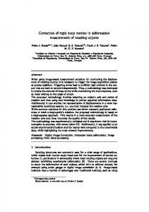
Figure 2.2: Performance-comparison of three popular physics engines (PhysX, Bullet and ODE) performed in [80]: 625 spheres were dropped onto a flat ground and the frame time in consecutive iterations was measured for each of the three engines. We can clearly see ODE being outperformed by the proprietary (closedsource) PhysX engine but it is no longer the case with open-source Bullet (based on Sequential Impulse algorithm) whose execution speed is comparable to PhysX. It is obviously an isolated test-case but shows that the quality offered by proprietary solutions is not completely beyond reach of independent developers. 2.2.2D

Closed-source engines

The two best known proprietary physics engines are PhysX and Havok. They have successfully dominated the market and are used in leading game engines and most popular games. Competing with these solutions is obviously a big challenge, especially in terms of feature richness, but the difference between these proprietary packages and community-created open-source solutions is not as great as one could expect (Fig. 2.2).

Chapter 3

Simulation of rigid body systems: foundations

3.1

Overview

This chapter is devoted to introduction of different aspects of rigid body dynamics and its basic mathematical description. Core terms and different high-level classifications along with principles of mechanics are provided without going into the details of methods or tools (even mathematical) used in simulation.

3.2

Non-interacting rigid bodies: projectile motion

A single rigid body in space has six degrees of freedom (DoF) which is equivalent to saying that in order to uniquely describe its configuration (i.e. position and orientation) one needs to provide six parameters: three for translation and three for rotation [78, 112]. What also follows is that the configuration space of a single rigid body is six-dimensional [78, 5]. Sometimes it is more convenient and intuitive to define the degrees of freedom as the number of basic independent motions that are possible to be made. The dynamics of a single rigid body is provided by the well known NewtonEuler equations; the momentum balance of a single rigid body is given by: f=

dl dt

(3.1a)

dh , (3.1b) dt where l and h are the linear and angular momentum of the rigid body, respectively; f and n are the net force and moment acting on the rigid body, n=

13

14

CHAPTER 3. SIMULATION OF RIGID BODY SYSTEMS: FOUNDATIONS

respectively. It is usually more convenient to use Eq. 3.1 expressed in terms of accelerations rather than momenta, but such a form is dependent on the choice of reference frame. If the equations are expressed about body’s center of mass and w.r.t. to an inertial frame, one obtains: f = mv˙

(3.2a)

n = Iω ˙ + ω × Iω,

(3.2b)

where m is the mass, I inertia tensor, v velocity and ω angular velocity. Eq. 3.2 is sometimes called the fundamental form of equations of motion [104]. If we can assume that a multibody system is a collection of rigid bodies that are perfectly independent (i.e. guaranteed not to interact) then we can simply treat each of these bodies as an isolated case. For n bodies, such a system has 6n degrees of freedom and configuration space of dimension 6n. System equations of motion (EOMs) are created by stacking/concatenating the equations for individual bodies: ¨ = f x + f v, Mq (3.3) where M is the system inertia/mass matrix, where q is the vector of generalized coordinates1 , f x is the vector of external forces acting on individual bodies and f v represents the velocity-product force terms, i.e. velocity-dependent terms2 depending on the choice of the reference frame and coordinates. Equation 3.3 is provided as one, composite system but there is no reason to use the multibody system EOM of in this form directly as long as there is no interaction between the bodies comprising it; each row of this system of equation can be treated interdependently (which has important practical implications when a parallel implementation is considered). The nice feature of multibody systems is lost once interaction between the bodies is considered.

3.3

Interaction

If the simulated multibody system is not just a set of permanently independent objects traveling along ballistic trajectories (projectile motion), means must be provided to allow for interactions between these bodies. The commonly distinguished cases of interaction are: • collisions 1 It means that q uniquely defines the configuration (i.e. positions and orientations) of bodies in the system. Some authors (e.g. [97]) further restrict the concept of generalized coordinates by requiring their number to be equal to the number of system degrees of freedom (which becomes important once constrained system dynamics are considered). However, we prefer the more general definition as provided by [120, 54, 64]. 2 Terms such as: inertia-variation term appearing as the second summand in the RHS of Eq. 3.2b; Coriolis and centrifugal terms in non-inertial reference frames.

3.3. INTERACTION

15

• resting contact • articulation • friction In the most basic terms, the task of the physics engine is to allow for this interactions while preventing inter-penetration.

3.3.1

Joints

Joints are permanent connections between bodies which by definition should not be allowed to disconnect. Rephrasing this in simulator terms: forces (called joint reaction forces) must be provided that prevent relative motion of the jointed bodies that would lead to violation of conditions imposed by a specific joint. As such, joint permanently reduce the amount of degrees of freedom for the system. Although jointed bodies are not supposed to inter-penetrate, the main consideration when designing joint models is preventing the articulation from falling apart rather than not allowing for the connected links to penetrate into each other. (examples?)

3.3.2

Resting contact

Resting contact is the type of interaction occurring when two bodies touch each other for some time. Unlike jointed bodies, the ones being in resting contact are allowed to disconnect at any instant, but (as with all the interactions) they are not allowed to penetrate into each other. Thus, the simulator must provide reaction forces that will prevent this from happening. This is a typical nonpenetration type of interaction, so the main consideration when modeling it is to prevent overlapping while not restraining separation (i.e. no sticking) of the bodies in contact. Another big issue in this context is handling friction.

3.3.3

Friction

The most famous and commonly applied law of friction is the one described back in 1785 [30] by Charles Coulomb. Ubiquity of the Coulomb’s law is probably due the simplicity and intuitiveness of its general principle along with the fact that it possesses the quality of being good-enough for the vast majority of applications. These features can be misleading though which has been succinctly and vividly summarized by Glocker in [101, Chap. 2]: With that friction law, one has chosen one of the most complicated force laws that occur in application problems. It seems to be so easy and so clear at a first view, however, when trying to apply it, or even when just trying to write it down as a mathematical expression, one

16


immediately encounters a lot of serious and not expected problems of very different nature. In its basic form, Coulomb’s law states that the friction force is bounded by the magnitude of the normal contact force (i.e. the one preventing penetration) times a certain scalar specific to materials of the contacting objects - coefficient of friction. If the contacting bodies are moving with respect to one another tangentially to the contact surface (i.e. sliding) then the friction force acts in the opposite direction of their relative tangential velocity (slip velocity)3 . If the slip velocity is zero only the magnitude of the friction force is determined by this law. Stated as above, Coulomb’s law can be summarized by the following formulae:   kv k = 0 t  kv k > 0 t

⇒

kf t k ≤ µkf n k

⇒

kf t k = µkf n k,

f t = −αv t ,

α ≥ 0,

(3.4)

where µ is the coefficient of friction, v t is the slip velocity, f n and f t are the normal and tangential components of the contact force vector, respectively. In the presence of sliding, friction is described as dynamic or kinetic; otherwise the term static friction (or sticktion) is used. Note that the static scenario includes the case of rolling and these terms are often used synonymously . Static and dynamic cases usually use separate friction coefficients: µ0 and µ for static and dynamic case, respectively, where µ0 > µ [5, 50]. The formulae in Eq. 3.4 are stated at the velocity level, but if one wishes to monitor transition from sticking to sliding it is convenient to consider the slip acceleration as well [52, 21]: the transition occurs when kv t k = 0 but kv˙ t k 6= 0. Usually, the direction of friction force in the instant of transition is required to directly oppose the slip acceleration [21, 49, 98], but some authors, e.g. [81, 82, 5, 6] provide a less restrictive version of the law: it is enough if the friction force is partially opposing the tangential acceleration, i.e. v˙ t · f t ≤ 0. 3.3.3A

Set-valuedness

Figure 3.2 depicts the above described dependence between the friction force and slip velocity in one-dimensional case. The first thing to notice is the fact that the illustrated force law is set-valued (at vt = 0 point), i.e. the force can take any value (in the allowed range) when there is no slip velocity. 3.3.3B

Problematic transitions

Different values of static and dynamic friction coefficients lead to a jump change when the transitions between these two cases occur. It can be avoided if they 3

The fact that friction forces are allowed to dissipate the kinetic energy due to slip velocity means that they are not workless (unlike contact normal and other constraint forces)[5]

17

3.3. INTERACTION

(a)

(b)

Figure 3.1: (a) Friction angle (2D), (b) Friction cone (3D); the relation with the coefficient of friction is µ = tan α

Figure 3.2: Friction force as a function of tangent/slip velocity (planar case)

are assumed to be equal at the instant of transition and more modern theories introduce the relation µ = µ(kv t k) thus allowing the coefficient of friction to smoothly depend on the slip velocity (Fig. 3.3) [50, 52, 113], which is experimentally grounded for most material pairings [52]. This approach eliminates another interesting/problematic feature of the model : while it is intuitive to assume that the friction force needs to reach the allowed bound before the stick-slip transition occurs, it is not the case for the opposite transition during which the force can step-change to any value in the allowed interval. This behavior is described as hysteretic by Glocker [50]. 3.3.3C

Non-linearity

More problems arise if we move to three-dimensional scenarios where the friction force is planar. In this case, the allowed contact forces (comprising both normal and friction components) are bounded by a so called friction cone (Fig. 3.1b)

18


Figure 3.3: Possible dependence of the friction coefficient, µ, on the slip velocity magnitude, vt [113] containing the admissible contact force vectors (i.e. sums of normal and frictional contact forces), which is usually given as follows: F C(q) = {f t + f n | kf t k ≥ µkf n k, f t ⊥ f n },

(3.5)

where q is the current system configuration , f t and f n are the tangential and normal components of the contact force, respectively and µ is the friction coefficient. Since the relation 3.5 incorporates the magnitudes of the 2D force vectors it is obviously non-linear, which makes handling of friction in 3D systems much more complex than in the planar case. Moreover, anisotropic friction is also possible in 3D scenarios4 [114]. 3.3.3D

Coupling

While the models describing normal and frictional contact forces are specified separately, the coupling between them is their intrinsic feature - a precise overall contact law cannot treat them separately5 . Apart from being more difficult to model in general, the coupling can lead to feedback effects between these components so strong that one needs allow for impulsive forces in the absence of collisions to provide a solution (Painlevé’s paradox) [5, 113].

3.3.4

Collisions

In reality, all bodies are deformable [23], but the idealistic assumption of perfect rigidity is very much justified for modeling bodies whose deformations and their influence on the motion of a body as a whole are negligible most of the time. However, the situation is quite different when it comes to collisions for which the fact of disallowing deformations changes the dynamics to an extent which needs special treatment (velocity is no longer a continuous function of time). To 4 The friction cone is then elliptic as opposed to the circular cone corresponding to isotropic friction [2]. 5 However, many approximate methods are based on the principle of handling these components separately.

19

3.3. INTERACTION

alleviate this without scarifying the assumption of rigidity, it is usually extended by a set of rules which guide the simulation through collisions [87, 23]. Such extensions are called impact or restitution models or hypotheses. When two rigid bodies come into contact (collide) an instantaneous stepchange of their velocities occurs which results in a discontinuity that cannot be expressed using an acceleration-level EoM6 due to the level of indirection between applied force and resulting velocity alteration. Step-changes in velocity/momentum can be expressed, however, using impulses - time-integrals of forces: Z t0

f (t)dt,

p=

(3.6)

t1

which have the effect of modifying the momentum as follows: Z t0

f (t)dt =

p=

Z t1 dh t0

t1

dt

dt = h(t1 ) − h(t0 ).

(3.7)

This relation is general and simply summarizes the effect of any force acting over a specific period. However, in the case of rigid collisions it allows for escaping the problem of an infinite force active over an infinitesimal time period; it is achieved by representing the effect of such a force by the following finite impulse: p = lim

Z t0 +δt f (t)

δt→0 t0

δt

dt.

(3.8)

What is also important in the case of rigid body collisions, as the time of application tends to zero, the effect of all finite forces is negligible. Impulses of this specific kind are sometimes called collision impulses and this convention shall be adopted in this work to differentiate them from any impulse as defined by Equation 3.6. Additionally, the name instantaneous impulses shall be used as well to stress the fact of the infinitesimal time of application characterizing them. . Like in the case resting contact, this is a non-penetration type of interaction: the main consideration when modeling collision is preventing overlapping without sticking and trying to incorporate friction. What is more, restitution law must be chosen and properly modeled which allows to resolve the collision in order to determine post-collision velocities of the colliders. 3.3.4A

Restitution laws

Let us first quote Chatterjee & Ruina [25] in order to define a restitution law (which they call a collision law) Given a pair of colliding rigid bodies (or mechanisms composed of rigid bodies connected with frictionless geometric constraints) in known 6

The force needed to produce the large acceleration diverges to infinity while the period of its application converges to zero

20


configurations and with known pre-collision velocities, and given the relevant parameters (which could be coefficients of friction, restitution, material properties, geometric information like local surface shape, etc.) a collision law predicts the contact impulse. The quoted work along with [24] by the same authors provide a richly referenced classification of different restitution law, which is however beyond the scope of this dissertation. As it was mentioned before, when two physical bodies collide, they keep deforming until the normal component of their relative velocity, vn , vanishes and the reaction force reaches its peak value7 ; this is called the compression phase (time interval [t− , tc ]). When the velocity changes sign, the restitution/decompression phase (time interval (tc , t+ ]) begins when bodies deform toward their original shapes, but will generally not reach it due to smaller compliance than during compression [117]. It is important to consider energy transformations as well: • during compression contact force changes the kinetic energy of relative motion into the internal energy of body deformation • during restitution the elastic strain energy accumulated in the previous phase generates force which drives the bodies apart which restores a fraction of the initial kinetic energy (rebound) [117]. This is obviously a very complex process and the restitution laws provide means to approximate it. The most famous and simplest among these laws is the one due to Newton: vn (t+ ) = −vn (t− ), (3.9) where the scalar value is called the coefficient of restitution. As one can see, the division of a collision into phases is not manifested in this formulation: we get a simple mapping from pre- to post-collision velocity. An alternative proposition known as Poisson’s restitution law/hypothesis can be perceived as a slightly more realistic model since it explicitly utilizes the concepts of compression and restitution phases by relating the impulse generated during their courses as follows: pn (t+ ) − pn (tc ) = pn (tc ),

(3.10)

where pn (ti ) represents the impulse of the normal force acting over the time interval [t− , tc ]. Eq. 3.10 states that the normal component of the collision impulse delivered during restitution is times what has been delivered during compression. However, the practical difference between Newton’s and Poisson’s hypotheses is 7

These events coincide in time [117].

21

3.3. INTERACTION

not that big since they are actually equivalent for frictionless collisions and when friction is present they can both cause the total energy of the colliding bodies to increase during a collision [87]. The energetic reformulation of the coefficient of restitution due to Stronge [117] relates the energy released during restitution with the energy that has been stored/absorbed by deformation during compression [124]; expressing it in terms of work done by normal components of contact impulses, Wn (t), one obtains [87]: Wn (t+ ) − Wn (tc ) = −2 Wn (tc ).

(3.11)

Eq. 3.11 ensures that normal contact forces will not add energy to the system, i.e. they are always dissipative (like frictional forces). 3.3.4B

Collision with friction

When resolving collisions it is often necessary to take friction into account and the usual choice is the Coulomb model. However, Coulomb law is formulated for the instantaneous values of contact forces and it cannot be simply assumed to hold for impulses which represent the total force acting over the collision timespan and thus a dedicated procedure for analyzing this process is needed. The over a century old treatment of frictional collisions by Routh is still commonly cited and one often encounters statements that not much has been done in this field since then [89, 124]. Routh used differential equations to describe the collision process [87] and developed a graphical method of analyzing it. Friction models used in contemporary interactive physics engines rarely go beyond the (simplified) Coulomb law and thus detailed description of frictional collisions is beyond the scope of this dissertation, but the relatively recent works like [25, 24] are a good resource on this and related subjects.

Chapter 4

Simulation of rigid body systems: methodology

4.1

Overview

The current chapter is an approach at extracting the relevant essence of the rigid body dynamics simulation state of the art without focusing on the works of specific authors who have contributed to it. It presents practical interpretations, proposed representations and tools (both mathematical and algorithmic) needed to build numerical simulators capable of generating rigid body systems motion approximating or directly following the principles introduced in Chap. 3. It discusses three main approaches to constrained multibody system modeling and simulation, i.e. penalty-based, constraint-based and collision-based methods.

4.2

Penalty-based methods

This approach provides the simplest means to introduce inter-body interactions into the model. Although particular realizations will vary in details, reaction forces are generally determined using stiff springs (Hooke’s law): the greater the configuration error the stronger the correcting/restoring reaction force. The spring is usually combined with a damper/dashpot to make the restoring force penalize velocity and thus reduce oscillations1 . Due to the simplicity of the underlying principles, ease of implementation and visually plausible animations penalty-based methods were widely used in the past [128, 91, 118, 53, 77, 105, 71] and are sometimes encountered in more recent works as well [88, 59, 130, 32, 1

Moreover, the damper has the additional effect of eliminating invalid velocity, e.g. if two bodies have already penetrated into each other it is incorrect for their velocities to keep increasing the inter-penetration.

23

24

CHAPTER 4. SIMULATION OF RIGID BODY SYSTEMS: METHODOLOGY

58, 84, 75]. Another advantage of penalty-based methods is that they generate physically valid reaction forces which cannot be always guaranteed by more advanced techniques: a canonical example is a symmetric table positioned on a flat ground2 [5, 87]. Naturally, if penalty-based methods met all the needs of the computer animation community, the research on interactive rigid body simulation could have been abandoned years ago. The following paragraphs briefly discuss the reasons why it did not happen. Configuration errors Since penalty-based methods generate reaction forces after invalid configurations have been detected, the simulation/animation based on them will suffer from from errors by definition. However, it is very often tolerable (to a certain extent) in the computer animation domain3 and can rarely be eliminated entirely, even if much more complex methods are used. On the other hand, the error must be kept relatively small to maintain the illusion of correctness which requires high spring constants; stiff springs make maintaining simulation stability harder. Tedious tuning It is very hard to provide a generally applicable and robust way of determining spring constants; they are usually found using ad hoc rules of a thumb which essentially boils down to tedious trial and error: • if constants are too low the visual artifacts become more and more visible • if constants are too high the resulting equations can become too stiff and thus hard to handle numerically (integration); the problem becomes more challenging with the growing number of interactions and can easily become intractable. Moreover, if for any reason the configuration error has grown very high (e.g. discrete collision detection along with a large simulation step), the parameters that are tuned to keep the error small can make the simulation unstable. Oscillation The fact that a configuration error must occur before any reaction force can be generated, the simulated bodies will tend to oscillate around the proper configuration (see Fig. 4.1) [32, 16]; this problem can be tackled by introducing the 2

The same acceleration of the chair’s center of mass can result from infinitely many distributions of the net ground reaction force on the legs and penalty-based methods produce physically intuitive results which is not guaranteed by the constraint-based methods [87]. 3 This is obviously not a general claim and surely not applicable in other domains, e.g. mechanical engineering.

4.3. CONSTRAINT-BASED METHODS

25

Figure 4.1: The problem of a body oscillating around the proper configuration inherent problem of penalty-based methods aforementioned dampers but it is hardly physical and generates even more parameters to tune.

4.3

Constraint-based methods

The interaction between the bodies comprising the systems limits their mobility so in general each body can (at least temporarily) have less than 6 DoFs. Those mobility limitations can be expressed in terms of constraint equations/inequalities, algebraic or differential equations/inequalities on position/orientation variables and/or their derivatives, augmenting the basic (i.e. projectile motion/ballistic) ODEs. The effect of introducing these constraint equations/inequalities is the additional coupling between chosen dimensions of the system configuration space4 which makes them mutually dependent thus decreasing the number of system DoFs. In terms of system dynamics, this means that specific forces must act on the system to enforce those relations.

4.3.1

Classification of constraints

A constraint is described by an algebraic equation in the configuration and/or motion variables of the body or system and can be classified basing on the exact form of these equations. The general classification that is about to be provided is mainly based on [40, 10, 3] and is one of at least two commonly used in the literature. The choice is somewhat arbitrary and definitely subjective. Alternatives are briefly discussed afterwards. . We will start by discriminating between so called bilateral (given by equations) and unilateral (given by inequalities)5 constraints. The former correspond to permanent interaction between bodies which is never allowed to be interrupted; the latter arise when bodies can interact but can also become independent by 4

To be exact: constraint equations/inequalities which consider one DoF are not uncommon; joint limits are a perfect example: single DoFs can be temporarily locked/disabled whenever a joint is about to leave the admissible region of its configuration space 5 In fact, bilateral constraints are often called equality constraint and unilateral - inequality constraints.

26


separation (as far as the constraint condition is considered). Thus, a body subject only to a unilateral constraint undergoes a free motion in certain portions of its configuration space but becomes constrained when entering others . The name unilateral comes from the fact if bodies are supposed to be allowed to separate constraint force must not prevent it while still allowing for interaction if need be: it must act in one direction only. Correspondingly, bilateral constraint generates a reaction force which acts in both directions. Next we consider what gets constrained: if these are certain configurations that we wish to disallow, then the corresponding constraints are called geometric; if these are certain types of motion that are prohibited - we need to apply kinematic constraints. It is important to note that when disallowing configurations (by applying geometric constraints), we also eliminate certain types of motion but it does not necessarily work the other way round. In order to put it in mathematical terms, let us introduce geometric constraint function, φh : φh (q, t) = 0

(4.1)

and let us differentiate it with respect to time to obtain: n d ∂φh ∂φh X φh (q, t) = + q˙i , dt ∂t ∂qi i=1

(4.2)

which can be perceived as kinematic/velocity version of Eq. 4.16 Now, let us introduce a different constraint function, φnh , which (unlike φh ) is linear in the velocity variables before it is differentiated: ˙ t) = φ0nh + φnh (q, q,

n X

φinh q˙i ,

(4.3)

i=1

where φinh , are functions of time and configuration variables, q, only [40]. Equations 4.2 and 4.3 have the same algebraic form but the latter cannot be integrated to resemble the former in Eq. 4.1 because it is simply not a derivative of any function. Constraints which can be both geometric and kinematic are called holonomic while those which are only kinematic - nonholonomic. Finally, we shall discuss the dependence on time, or, to be more precise, explicit dependence on time. A constraint is called rheonomic if it is explicitly dependent on time and thus enforces prescribed motions. If there is no such explicit dependence, the constraint is called scleronomic. Unfortunately, various authors classify constraints differently and it is quite hard to choose the proper approach. Very often inequality constraints are treated as non-holonomic (by assumption that constraints that are not bilateral and holonomic are simply non-holonomic) [108, 33, 12, 3]. Furthermore, it is not always 6

Providing the kinematic version of the constraint equation in respected at all times.


27

clear whether one should use terms scleronomic and rheonomic in unilateral cases [90, 40]. Certain authors disassemble the classification hierarchy completely and propose to use the classes as a set of independent labels which (presumably) are applicable in any combination [48]. Luckily, this struggle for proper and clear distinction between different constraint types is not our concern. Thus, to avoid the needless confusion introduced by generalizing classifications, we will provide three classes of constraints typically encountered in physics-engines domain and only refer them to the formerly provided formal definitions. 4.3.1A

Joints

Joints generate bilateral holonomic constraint because the corresponding reaction forces can both push and pull in order to block the motion which would lead to disallowed configurations. Usually joints yield scleronomic constraints, but it is conceivable to treat them as rheonomic in kinematically-driven motion cases. 4.3.1B

Non-penetration

Non-penetration is obviously defined by providing valid and invalid configurations; furthermore, it is enforced by preventing motion in one direction of a chosen dimension since the reaction force can only repel, not attract. These two features mean that non-penetration requires holonomic unilateral constraints. Since time-controlled contact sounds grotesque, one can safely assume that these constraints are also scleronomic. 4.3.1C

Joint limits

To maintain generality, joint constraints are usually chosen from a moderate set of canonical models like hinge or ball-and-socket joints which correspond to relatively uncomplex configuration or motion subspaces. Joint limits enable customization of the standard models by explicitly specifying valid ranges of the configurations allowed by the joint. Human knee can serve as an example here (Fig. 4.2). General properties of joint limits are mostly the same as those characterizing non-penetration constraints. 4.3.1D

Velocity constraints

A good example of a velocity constraint is a requirement that wheels of a vehicle rotate with a specific angular velocity; velocity constraint says nothing about the configuration of these wheels. Therefore, when discussing velocity constraints, we need to consider valid and invalid velocities rather than configurations which clearly means we are dealing with nonholonomic constraints. However, it is hard

28


1 DoF

1 DoF

0 DoF

Figure 4.2: Knee modeled by a hinge joint and an additional limit to characterize this class any further since both unilateral and bilateral velocity constraints seem reasonable and, similarly to joints, in the case of kinematicallydriven motion they could well become rheonomic.

4.3.2

Constrained system EOMs

The unconstrained rigid body equations of motion presented by Eq. 3.6 will now be modified to (explicitly) contain the vector representing reaction forces of the constraints, f c : ¨ = f x + f v + f c. Mq (4.4) By the principles of virtual work (or power) [78, 112, 129, 65, 40] we can always express the constraint forces as follows: f c = J Tc λc ,

(4.5)

where J c is the Jacobian matrix of the constraint equation treated as a vectorvalued function of the system configuration vector, q . This Jacobian matrix is commonly referred to as a constraint Jacobian matrix (or shortly constraint Jacobian 7 ); if all the constraints in the system are bilateral J c is given by:  ∂φ1 ∂q1

Jc =

∂φ  .. =  . ∂q ∂φ

m ∂q1

··· .. . ···

∂φ1 ∂qn



..  .  ,

(4.6)

∂φm ∂qn

7 The nomenclature concerning Jacobian matrices is ambiguous: they are commonly referred to simply as Jacobians (especially among roboticists [31]), but so are their determinants! However, since Jacobian matrix determinants do not appear in this work, we shall adopt the convention of using the terms Jacobian matrix and Jacobian as synonyms.


29

where φ(q) is a bilateral constraints function. Let rows of J c be grouped by type and stored in smaller Jacobians: Γ , Z and Υ for holonomic, non-holonomic and unilateral constraints, respectively; the same holds for λ. These assumptions yield:     γ Γ     (4.7) J c = Z  , λc =  ζ  . υ Υ The deeper meaning behind the principle of virtual power and Eq. 4.5 is that constraint forces act so as to eliminate any illegal motions without influencing the legal ones. This condition is naturally fulfilled if in the system configuration space constrain forces, no matter their magnitudes, are oriented orthogonally to any valid velocity vector8 . Getting back to the equation of motion: inspecting the Eq. 4.5 we can say that if the constraint equations are known, so are the directions of the corresponding reaction forces. Therefore, what remains to be determined are only their magnitudes, λ. Now, substituting Eq. 4.5 into Eq. 4.4 one obtains: ¨ = f x + f v + J Tc λc , Mq

(4.8)

which is an undetermined system of ndof equations in ndof +nc unknowns: system accelerations and the magnitudes of reaction forces. Therefore, in order to fully determine it one needs to supply nc additional relations, which are specific to constraint types.

4.3.3

Joints

In case of joints their constraint equations seem like a natural candidate for making the system in Eq. 4.8 fully determined: ¨ = f x + f v + Γ T γ, Mq

(4.9a)

φ(q) = 0,

(4.9b)

where Eq. 4.9b represents the joint constraints. This choice yields a set of Differential Algebraic Equations (DAEs). DAEs combine differential and algebraic equations and are often viewed as differential equations on manifolds [47]. The formal definition of a DAE (in implicit form) is: F (t, z(t), z(t)) ˙ = 0,

(4.10)

where z denotes the state. If ∂F ∂ z˙ is non-singular then the above equation could be converted into an ODE [28, 47]. What follows is that explicit and implicit ODEs are special cases of DAEs [100, 47]. 8

It also means that constraint forces are not allowed to do work on the system - they are workless.

30


A DAE in a semi-explicit form can be written as: x(t) ˙ = f (t, x(t), y(t))

(4.11a)

0 = g(t, x(t), y(t)),

(4.11b)

where the state z is now split into components x and y called the differential and algebraic variable, respectively [47]. DAEs in this form are sometimes viewed as ODEs with constraints. In order to measure the difficulty (in terms of stability and accuracy) in the numerical treatment of different DAEs a notion of an index has been introduced which quantifies the degree of regularity of a DAE [47]. DAEs of index 2 or higher are called higher index DAEs. Several different index definitions have been proposed for general systems but they are way beyond the scope of this work. In our particular case, EOMs for a mechanical system subject to holonomic constraints form semi-explicit DAEs of index 3 [65, 21, 69, 19, 16] or, equivalently, Hessenberg DAE of index 3 [47], which means that the various index definitions coincide and thus it is typical to focus on the so called differential index only which is defined alternately as: • the minimum number of differentiations with respect to time of the algebraic equation 4.11b (followed by substitution of 4.11a for x) ˙ needed for the resulting equation to become solvable for y˙ [47, 65, 28] • the number of times the constraint equations need to be differentiated to obtain an ODE (called the underlying ODE)9 Solving general DAE systems is still a very active research area and the methods proposed so far are from achieving the maturity of corresponding ODE approaches [100, 21, 69, 65]. Numerical methods employed for DAEs belong to the group of either backward-difference (BDF) or implicit Runge-Kutta (IRK) methods but these approaches a far from being general or suited for real-time/interactive purposes [62, 65, 74]. A popular alternative for dealing with higher index DAEs is to reformulate them in order to obtain a more tractable lower index problem [69, 47], which can be achieved by differentiating the constraint equations with respect to time10 ; this method is called an index reduction of a DAE. However, although this simplification is analytically sound since the lower-index DAE has the same solution as the original one, it is no longer so in the case of a numerical solution [60, 47]. This results in accumulation of the error on configuration/position and/or velocity levels in the course of simulation and thus demands applying techniques 9

Note: since ODEs are actually special cases of DAEs [47] they are sometimes described as index-0 DAEs [47, 62, 65, 18]. 10 Each differentiation of the constraint/algebraic equations reduces the index by one [47].

31


minimizing/eliminating the visible artifacts [8, 60, 47, 27]. Let us apply the index reduction technique to the EOMs in Eq. 4.9; it requires us to differentiate the constraint equations with respect to time twice, which yields: Γ q¨ + Γ˙ q˙ = 0 ⇐⇒ Γ q¨ = −Γ˙ q, ˙ (4.12) and combine it with Eq. 4.8, to finally obtain index-1 DAE of the form : "

M Γ

−Γ T 0

#" #

"

#

q¨ f +f = x ˙ v . γ −Γ q˙

(4.13)

This equation is often called the descriptor form of the equations of motion [60] and the constraint force magnitudes are usually referred to as Lagrange multipliers thus referring to the well known mathematical optimization method dealing with extremizing a function subject to equality constraints. Another popular convention is to call this form of EOMs Lagrange equations of the first kind [17]. The system in Eq. 4.13 can be obviously solved directly, especially if the of constraint Jacobians and inertia matrix introduce a substantial level of sparsity [8] or it is possible to prune out of linearly-dependent rows [40]. Alternatively, one can subtract Γ M −1 times the first row from the second row to obtain equation: Γ M −1 Γ T γ = −Γ˙ q˙ − Γ M −1 (f x + f v ).

(4.14)

The coefficient matrix Γ M −1 Γ T is closely related to the inverse of the operational space inertia matrix introduced by [67] but a common convention for its name or symbol does not really seem to exist11 . For joint constraints, this coefficient matrix is always symmetric positive-definite [40], but not necessarily full-rank in which case least-squares solution is determined. Once the Eq. 4.14 has been solved for the multipliers γ, we can move back to Eq. 4.13 to compute accelerations. Another way to avoid DAEs arising due to holonomic constraints is to express the system dynamics in terms of its degrees of freedom; this approach is sometimes called the embedding technique [112] and the set of independent parameters used - the reduced coordinates 12 . Generally speaking, embedding eliminates the constraint equations and the corresponding reaction forces at the cost of increased complexity and nonlinearity of the equations13 [112] 11

To the best of author’s knowledge. Coordinates resulting from treating all bodies as free objects restrained by reaction forces are sometimes called the maximal coordinates 13 The increased complexity/nonlinearity should not be surprising since the same information must be expressed using a smaller set of equations [112] 12

32


The first step is to express the dependent coordinates in terms of the independent ones q = b(q r ), (4.15) where q and q r denote the maximal- and reduced-coordinate configuration vectors, respectively. A single time-derivation yields the following relation between velocities yields: ∂b r q˙ = q˙ = B q˙ r , (4.16) ∂q where B is the velocity transformation matrix[112]. The important feature of B is the fact that if f c denotes the reaction forces of the constraints enforcing the relation in Eq. 4.15, then using the principle of virtual power one can prove that B T f c = 0. Let us differentiate Eq. 4.15 w.r.t. time once again to obtain acceleration-level relation: q¨ = B¨ q r + B˙ q˙ r , (4.17) substitute it into Eq. 4.4 for x ¨: M B¨ q r = f x + f v + f c − M B˙ q˙ r

(4.18)

and left-multiply it the resulting expression by B T to eliminate the reaction force vector, f c : B T M B¨ q r = B T f x + B T (f v − M B˙ q˙ r ) = ¨ r = f rx + f rv , = M rq

(4.19)

which is an EOM of the system in terms of its degrees of freedom. The Lagrange-multiplier-based methods and the embedding technique have their advantages and disadvantages which in many cases complement each other. Lagrange multipliers: pros and cons The multiplier approach is intuitive, yields relatively simple and thus legible equations; adding/removing constraints is straightforward which facilitates software design. On the other hand, there are two basic problems with this approach: • reducing system degrees of freedom makes the system to be solved larger; in cases when most DoFs are permanently eliminated this approach may not a good choice performance-wise • index reduction when faced with the inherently imprecise/approximate nature of the numerical integration process causes the configuration error to accumulate over time resulting in what is popularly known as the drifting problem of multiplier approaches

33


Reduced coordinates: pros and cons The situation is perfectly opposite in the case of reduced coordinates: they yield more complex equations and they are commonly believed to be more difficult to understand and implement. Furthermore: • means must be provided to define the proper set of independent variables; while this is quite easily achieved if the underlying topology is a tree, but providing a general solution is very difficult and rarely practical for general purpose simulators • determination of the coefficients of the EOM will in most cases require more complex algorithms than in the multiplier approaches • reduced coordinates cannot be used to express non-holonomic constraints (as opposed to multiplier methods) [8] The advantages of reduced coordinates are: • they are free from the drifting problem • more constrained systems yield smaller EOMs: every new constraint decreases the number of DoFs which reduces the dimension of the EOM to be determined and solved

4.3.4

Velocity constraints

Introducing this type of constraints into the EOM is done very similarly to the joints’ case: ¨ = f x + f v + Z T ζ, Mq

(4.20)

Z q˙ = 0.

(4.21)

Again, with this approach we end up with a semi-explicit DAE, only this time it is index-2 [69, 62].

4.3.5

Non-penetration

If one wishes to introduce non-penetration constraints turning the Eq. 4.8 into a fully determined system requires more consideration. The basic problem here can be summarized by the following relation between the value of a scalar nonpenetration constraint function, ψ(q)14 , and the corresponding normal contact force preventing the penetration (given by its scalar Lagrange multiplier, λ): λ ≥ 0, 14

ψ ≥ 0,

λψ = 0,

(4.22)

Dependency on the system configuration vector, q, is often dropped for convenience; we shall follow this convention.

34


Figure 4.3: Corner law illustrating the complementarity between the normal components of the acceleration, an , and contact reaction force, fn . which is often referred to as Signorini’s conditions/law or a corner law for normal contacts [20, 102, 21, 103, 127] (Fig. 4.3). The two inequalities in Eq. 4.22 manifest a convention stating that valid (by their physical interpretations, see below) values of both λ and ψ are non-negative, which must guaranteed by proper choice of coordinate frames and constraint equation/function. The third relation is known as a complementarity condition which requires at least one the two factors, λ and ψ, to be zero at all times. The intuitive physical interpretation of Eq. 4.22 is that either: (i) the bodies are in contact and thus ψ = 0 and the reaction force is allowed to act (λ ≥ 0), or (ii) there is no contact which yields ψ > 0 and therefore the reaction force must be zero (λ = 0). It is thus apparent that the condition Eq. 4.22 can be used as an indicator of the contact transition phases. If the normal relative distance between two formerly non-contacting bodies becomes zero, the contact is said to have become active and an appropriate normal contact force must be provided. If, on the other hand, the constraint force preventing penetration of two formerly contacting bodies becomes negative (change from repulsive to attractive) it means that detachment is occurring and the contact is said to have become passive. [102] Simply monitoring these indicators is an obvious approach for single-contact scenarios but it is known to become intractable as the number of interdependent contacts grows [102, 21]. As noted by Delassus, this leads to a massive combinatorial problem of testing 2m combinations (m is the number of contacts). Therefore, a non-naive approach is necessary. In the case of multiple contacts Eq. 4.22 becomes: λ ≥ 0,

ψ ≥ 0,

λT ψ = 0,

(4.23)

35


where the vector inequalities should be understood component-wise. Eq. 4.23 is often phrased briefly as: 0 ≤ λ ⊥ ψ ≥ 0. (4.24) Posing the conditions in Eq. 4.24 is equivalent to defining the set of admissible normal contact forces [44]. If there are only unilateral constraints in the system its dynamics are given by: ¨ = f x + f v + Υ T υ, Mq

(4.25a)

0≤υ⊥ψ≥0

(4.25b)

Complementarity between the position-level constraint, ψ, and corresponding reaction forces is always true but different conditions are also possible and often more convenient for analytic or numerical treatment of multi-contact scenarios [20, 21]. Let us first define a non-penetration constraint at velocity and acceleration levels. The former is obtained by differentiating ψ once with respect to time: ψ˙ = Υ q˙ ≥ 0,

(4.26)

ψ¨ = Υ q¨ + Υ q˙ ≥ 0.

(4.27)

and the latter by doing it twice:

d2 ψ

¨ ψ˙ = dψ dt and ψ = dt2 are the relative normal velocity and acceleration corresponding to the non-penetration/contact constraint ψ, respectively. Let us assume that there was a contact between two bodies and it was broken at time t0 : ψ(t < t0 ) = 0, ψ(t0 ) > 0. (4.28) From the definition of a derivative15 it follows that for a non-zero time interval [t0 − v , t0 ) the normal contact velocity must have been positive [81]. Using the ˙ same logic, assuming that ψ(t) is continuous and: ψ(t < t0 ) = 0,

˙ < t0 − v ) = 0, ψ(t

ψ(t0 ) > 0,

˙ 0 − v ) > 0, ψ(t

(4.29)

one can conclude that for a non-zero time interval [t0 − a , t0 − v ), a < v the relative normal acceleration must have been positive. In fact, this logic can be extended to derivatives or arbitrarily high order [20, Remark 5.14]. It is therefore possible to state the complementarity condition between force and velocity or acceleration (which is very popular in the literature) but it is important to note that different level complementarity conditions are not exactly equivalent to the original position-level one [20, Remark 5.14]. 15

And because x(t) (and thus ψ(x)) is obviously continuous

36


Let us limit this general discussion to acceleration-level complementarity for now (other options will be covered later). For multiple interdependent contacts it can be written as follows: ¨ ≥ 0. 0≤υ⊥ψ

(4.30)

The main advantage of applying complementarity at this level is the fact that it can be directly used to augment the constrained system EOM (Eq. 4.8) in order to obtain a Linear Complementarity Problem (LCP). Indeed, performing the same substitution as in the case of holonomic constraints, i.e. using Eq. 4.8 to eliminate x ¨ from Eq. 4.27, and then combining the result with the conditions 4.30 leads to:  ψ ¨ = Υ M −1 (f + f ) + Υ M −1 Υ T υ + Υ˙ q˙ x v  υ ≥ 0, ψ ¨ ≥ 0, υ T ψ ¨ = 0,

(4.31)

which has the structure y = Ax + b,

y ≥ 0,

x ≥ 0,

y T x = 0,

(4.32)

known as an LCP in the standard form [52, 94, 29]. Obviously, the coefficient matrix A has the same meaning as its holonomic counterpart in Eq. 4.14

4.3.6

Acceleration- or velocity-level

The basis of the traditional modeling techniques is the usage of second order differential equations of motion. Since this view relates forces/moments acting on the system with system accelerations it is sometimes called the force-acceleration scheme [21] or model [116]. EOM stated at this level provides an instantaneous view on the system: the simulation sets up these equations at each discrete moment in time in order to solve them for system accelerations (and possibly unknown reaction forces). The determined accelerations are then used to advance the simulation in time by means of a numerical integrator [2], which is roughly equivalent to stretching the discrete instant over a non-zero time interval. The obvious problem with acceleration-level approaches is that they cannot really handle collisions - the continuity of velocities is implicit into this formulation/only finite reaction forces can be determined . In order to enable simulator based on this approach to handle collisions a special treatment is needed: whenever a collision event is detected the flow of the simulation is interrupted to handle it using a collision impulse and an impulse-momentum/velocity relation; once all collisions are resolved this way, the simulation is restarted with the modified state. This technique, which is sometimes called an event-driven approach


37

to collisions/nonsmooth motion [93, 21], may seem like an ad hoc approach but is actually well-based in terms mathematical descriptions of nonsmooth motion (see Sec. A.2). This is sometimes pointed as on of the arguments against using acceleration-level formulations. The main drawback of acceleration-level approach occurs when modeling contact using LCP. For frictionless contact, an acceleration-force level LCP is known to have a solution (not necessarily unique) [5]. However, in the case of frictional contact, only certain special cases are guaranteed to be solvable; there are wellknown configurations (including single-contact scenarios, e.g. Painlevé’s paradox) for which accelerations consistent with the contact constraints do not exist [2]. One way to overcome the problem of acceleration-level formulation is to discretize the EOM before solving it for accelerations (instead of solving them as a differential equation and discretizing/numerically integrating then ). In other words, the acceleration determination step is combined with the velocity update which is probably why methods based on this approach are very often called time-steppers. In this formulation, system dynamics are expressed by a difference equation relating impulses (time integrals of forces) and velocity increments rather than a differential equation relating forces and accelerations. Therefore, we are no longer observing the system at a single time instant but rather over the time-interval of integration. Advantages of the velocity-level formulation over the accelerationlevel include: • it solves a much wider class of problems thanks to allowing friction to cause discontinuous velocity jumps in the absence of collisions • they handle finite and infinite forces in a unified fashion16 • velocity-level algorithms are amendable for convergence analysis, which is not the case for acceleration-level alternatives [21]

4.3.7

Handling friction

Since the dominating approach in constraint-based methods is to formulate an LCP, the chosen friction law, Coulomb or its approximation in majority of cases, also needs to be tailored in order to fit the formulation. Means used to achieve this vary considerably as different authors allow different levels of approximation and generality. Therefore, in the following section we shall try to provide the main tendencies without going into details of specific realizations. The first commonly applied adjustment of the Coulomb law is the approximation of the friction cone (Eq. 3.5) with a polyhedral one, which is necessary 16

There is no direct way to tell whether an impulsive force has acted over the time-step [115].

38


to avoid non-linearities yielding an NCP rather than LCP. The simplest possible polyhedral cone is a four-facet pyramid; the more facets are introduced, the closer we get to the original cone at the expense of simplicity (i.e. in general, more computations need to be performed). 4.3.7A

Acceleration-level

Dynamic friction Let us first assume that all the contacts in the system yield dynamic friction only. Therefore, just as in the frictionless case, the only independent values that need to be determined are the normal components of contact forces since the tangential ones are then uniquely determined by slip velocities (provided by the system state) and coefficients of friction. What is more, the entire problem can still be expressed in the general form of an LCP. The problem which arises in such a setting is that the coefficient matrix is no longer symmetric which means that the LCP is no longer convex: finding solutions to non-convex LCPs is NP-hard. Furthermore, the existence and uniqueness of reaction forces solving the problem at the given time is not guaranteed. Static friction Including the static friction requires more preparation. First of all, when working at the acceleration level the case of zero slip velocity requires further specification w.r.t. slip acceleration, v˙ t : • v˙ t = 0, i.e. the friction remains static • v˙ t 6= 0, i.e. transition to sliding is occurring As discussed before (see 3.3.3B), it is commonly (realistically) assumed that the static and dynamic friction coefficients are equal at the instants of stick-slip/slipstick transitions. We can illustrate the slip acceleration-friction force relation using the Fig. 4.5 it is apparent that the relation is more complex than the corner law presented before17 (Fig. 4.3). A common approach to deal with this, is to introduce slack variables in order to decompose the characteristic so that each component is equivalent to the corner law, but their intersection yields the original relation for static friction. Different decompositions are possible, but the simplest one is enough to convey the essence of these approaches: • friction is isotropic and its cone is approximated by a pyramid (i.e. its basis is a square and the slip accelerations/friction forces are represented by 2D vectors) 17

It is sometimes called the double-corner law [103].

39


Figure 4.4: Tangential characteristic illustrating the relation between the tangential components of relative acceleration, at , and and contact force, ft • each component of v˙ t is decomposed into its non-negative and non-positive parts, v˙ t+ ≥ 0 and v˙ t− ≥ 0, respectively such that v˙ t = v˙ t+ − v˙ t− • for each component of the friction force two slack variables, s+ ≥ 0 and s− ≥ 0, are introduced such that s± = µfn ± ft ; s+ (s− ) is positive as long as ft is negative (positive) and inside the friction pyramid; when it vanishes sliding can begin18 Under the above assumptions, static friction can be stated using the following complementarity relations which should be appended to the normal component conditions: 0 ≤ s+

⊥

v˙ t+ ≥ 0

and

0 ≤ s−

⊥

v˙ t− ≥ 0,

(4.33)

for each static contact and both of its tangential directions. The decomposition process is illustrated in Fig. 4.5. Still, the ability to cast the frictional contact problem as an LCP does not change the fact that the class of scenarios solvable at the acceleration-force level is very limited. Let us thus proceed to velocity-level formulations. 4.3.7B

Velocity-level

For velocity-level formulations it is typical to resolve friction conditions at the end of the time step, so there is no initial discrimination into static and dynamic friction contacts. On the other hand, there is no slip acceleration to be 18

These slack variables are sometimes called the friction saturations [52] and, colloquially speaking, quantify how much the current friction force is away from its maximal or boundary value. The transition to sliding is possible if they vanish.

40


Figure 4.5: One of the possible decompositions of the tangential characteristic in Fig. 4.4: tangential component of the relative acceleration, at , is split into its non-negative and non-positive parts tracked. Therefore, although decomposition into complementarity conditions is also applied, its role is a bit different: it must encompass the entire velocity-level Coulomb law. What may be surprising is that if we drop the distinction into dynamic and static friction coefficients (a common simplification [115, 2, 1, 110, 33]), the simple decomposition rule described in the previous section can be directly applied at the velocity level by substituting the slip accelerations with slip velocities.

4.4

Collision-based methods

Unlike constraint-based approaches, collision-based methods19 do not apply explicit algebraic constraints on the configuration of bodies in the simulated system. All interactions are handled using collision impulses. Between the collisions/interactions bodies act independently following ballistic trajectories. The need for algebraic constraint conditions on the configurations of interacting bodies is omitted by treating interactions locally, i.e.: • only a single pair of bodies is analyzed/handled at a time • no macroscopic assumptions about the nature of the currently analyzed interaction are assumed; the proper macroscopic behavior is supposed to 19

These methods are most commonly known in the literature as impulse-based, which is however (in the author’s opinion) quite misleading since impulses by their definition (i.e. timeintegrals of forces) are not specific neither to this approach nor to the case of rigid body collisions.

4.4. COLLISION-BASED METHODS

41

result from proper model/application of impact laws The above description defines what one might call a purely collision-based simulator and is provided in this manner to distinguish it among other approaches (the need which is often overlooked in the literature). As such, however, despite being valid and practically proven approach, has a limited application domain and one needs to relax some of the assumptions to be able handle broader range of systems. Therefore, collision-based simulators are usually equipped with elements typical for the constraint-based methods to make the best of both worlds, but their exact classification is hard since the borders between different paradigms become blurry. We shall call such hybrids collision-constraint-based simulators.

4.4.1

Resting contact and joints

The problem that naturally arises with collision-based methods are the ways of treating the resting contact. While in principle it could be resolved by series/trains of collision impulses, it is computationally inefficient in most implementations20 whose authors are thus forced to discriminate between the cases of resting and colliding contact and treat them separately. The situation is even worse with joints: a simulator which expects bodies to be connected by precise joint geometries in order for it to provide articulation based on detecting and resolving collisions is easily conceivable, but chances for making it work in interactive rates for massive multibody systems is not likely to become feasible in the near future. Collision-constraint-based simulators can treat the system in the collisionfree intervals as an articulated structure rather than a set of independent rigid bodies [86, 87] by applying any of the well known algorithms suitable for modeling the continuous motion of such systems. For animating jointed structures this technique is definitely a more tractable approach than purely collision-based methods, but may raise questions on how it differs from acceleration-level simulation restarted after collision is detected to apply impact dynamics (see Sec. 4.3.6). Alternatively, joints and contact can be simulated by applying impulses to eliminate disallowed velocities, which can naturally lead to error accumulation due to drift. Another hybrid technique is to apply collision impulses at the beginning of the time step such that the resultant velocities guarantee no configuration error (within tolerance) at its end [13, 126].

4.4.2

Handling friction

As mentioned in section 3.3.4B, Coulomb law is formulated for contact forces and does not simply generalize to impulses. However, many authors dealing with 20

It becomes apparent when one considers collision-based methods using CCD: for continuous contact the time of impact estimates tend to zero bringing the simulator to a halt [87].

42


A

B

Figure 4.6: An unstabilized simulation of a swinging pendulum [27]; the solid curves illustrate the trajectories of the pivot point, A, and center of mass, B frictional collisions ignore the fact which is usually enough to provide plausible animations, but can lead to energetic inconsistencies [21]. The impulsive Coulomb law along with another simplification - assumption of constant sliding velocity direction across the collision - form the basis for most of the simulators designed for computer graphics with the noteworthy exception of [87], who approached the collision resolution process utilizing methods similar to Routh and applied the Coulomb model for the time-derivatives of impulses (i.e. forces).

4.5

Fighting configuration errors

Minor configuration errors are sure to occur no matter which simulation paradigm is chosen, either due to the core properties of the chosen methods or simply because of to the finite precision the computer arithmetic. Therefore, the problem discussed in this section is thus not whether incorrect configurations will occur but whether the chosen simulator realization is capable of eliminating it before it is noticeable without deteriorating the stability or quality of the simulation.

4.5.1

Penalty-based methods

Configuration error is an inherent feature of penalty-based methods and the only thing one can do is to keep it as small as possible by properly adjusting spring and damper parameters or decreasing the simulation time-step.

4.5.2

Constraint-based methods

The main source of error in the case of popular constraint-based methods is the approximate nature of numerical integration. Most of the interactive constraintbased simulators enforce the geometric/configuration constraints only by ensuring

4.5. FIGHTING CONFIGURATION ERRORS

43

the velocities/accelerations does not lead to their violation21 (see Sec. 4.3.3); once those correct velocities/accelerations are numerically integrated to update system state, configuration errors are introduced [8, 27]. One can obviously decrease the integration time-interval or choose a higher order integration scheme but firstly: it will never eliminate the error entirely, and secondly: it increases the time of execution making it inapplicable in the interactive simulation realities [27]. The process of tackling constraint configuration errors is commonly called the constraint stabilization. The simplest and most common constraint stabilization technique is the so called Baumgarte stabilization: let us assume that we are dealing with a joint constraint and thus its acceleration-level equation is given by Eq. 4.12; if we assume that e denotes the configuration error then Eq. 4.12 is the following differential equation: e ¨ = 0. (4.34) Baumgarte stabilization replaces the acceleration-level constraint above equation by [40, 112, 65]: e ¨ + 2αe˙ + β 2 e = 0, (4.35) which combined with by Eq. 4.12 leads to: Γ q¨ = −Γ˙ q˙ − 2αe˙ − β 2 e

(4.36)

and is equivalent to introducing a damped-spring-based penalty force acting so as to eliminate the error term e. Therefore, Baumgarte stabilization suffers from the same problems penalty-based methods do. One final note is that the Eq. 4.35 applies to acceleration-level formulations; the velocity-level counterpart uses only the β 2 e term since the solver itself corrects the velocities. The problem with the Baumgarte stabilization is the fact that it introduces energy into the system. To avoid correcting the error by modifying the EOM one can project the solution onto the valid manifold in the configuration space after each time step [125, 1, 116]. This technique is sometimes called poststabilization [125, 27]. Let us assume that the configuration level constraint equation is g(q) = 0; the idea is to find a smallest possible corrective term, dq, such that while g(q) 6= 0 (i.e. q has drifted away from the constraint manifold), g(q + dq) = 0. This approach relates forces/impulses with configuration increments directly and is thus sometimes compared to a so called first-order world which assumes velocities to be driven by forces [7, 33]. Researchers have proposed to determine the corrective terms solving non-linear equations [1], an approximate linear system [7] or an LCP [27]. Finally, one can try to create a solver aware of the configuration-level constraint conditions and thus reacts to configuration errors before they manage 21

Except the constraints introduced by the embedding technique.

44


to accumulate. This may sound like the return to higher-index DAEs which does not seem a practical approach for interactive simulators but is not necessarily the case. Certain researchers have turned their attention to the concept of pre-stabilization: the configuration error for each constraint at the end of the time-step is first predicted and then a correcting impulse is determined. This, however, requires solving a set of nonlinear equations [125, 126] or a less precise linear approximation [15, 14]. See Sections 5.2.7 and 5.3.7 for more details. Moreover, one of the best-known time-steppers [115] enforces non-penetration at the configuration level which results in a non-linear complementarity problem (See Sec. 5.2.3) which seems to deter the interactive simulation community.

4.5.3

Collision-based methods

Purely collision-based simulators are not really designed to handle penetration: the entire idea is to model local interactions very precisely. Therefore, different approaches at continuous collision detection (CCD) are typically applied, which essentially boils down to either predicting the time of impact or backing-up the simulation to the approximate time of collision once penetration is detected. If discrete collision detection is used or in the case of collision-constraint-based hybrids one can obviously apply the same techniques as those described in the previous section.

Chapter 5

Literature survey

5.1

Overview

Basing on the general introduction of the methodology provided in Chap. 4, several prominent works in the field of rigid body simulations will be summarized and categorized in the current chapter. Note that the surveyed works will be discussed in varying detail since they differ in both their impact and fitness for brief presentation1 .

5.2

Unilaterally constrained systems

Frictional contact and collision seem to be the single most difficult interaction types to simulate and have thus attracted a lot of scientific attention among researchers in the fields of mathematics, mechanics, robotics and computer graphics. If, however, one looks upon related publications from the last three decades it turns out that the path to the contemporary interactive simulator can be interpolated using the works of less than ten authors. Formulating contact problems in terms of LCP has gained a lot of popularity in 1980s and 1990s. Casting the constrained system dynamics as an LCP enabled unilateral constraints to be posed directly rather than by bilateral constraints switched whenever attractive contact reaction force was detected [61]. The earliest description of a simulator using constraint-based methods to calculate reaction forces (by quadratic programming) appears to be by Lötstedt [81, 82]. The next prominent contributor in this stream of research is definitely Baraff who after several earlier research and survey papers wrote an easy-toread paper on modified Dantzig’s LCP solver [6] applied to enforce frictional 1

These are obviously subjective criteria.

45

46

CHAPTER 5. LITERATURE SURVEY

non-penetration constraints. Due to the limited range of problems solvable by acceleration-level formulation, certain authors ([115, 2, 110]) have turned their attention to velocity-level constraint-based methods whose origins date back to the works of Moreau [93] and Monteiro-Marquez [85]. In recent years, there has been a noticeable shift towards collision-based approaches and their fusions with velocity-level constraint-based methods [89, 86, 55, 111, 13, 15, 14, 126, 11] which was strengthened by the fact the the general simplicity and robustness of these algorithms resonated with physics engine developers.

5.2.1

Lötstedt

The works of Per Lötstedt starting from late 1970’s and through early 1980’s are often referred to as pioneer in the field of rigid body systems simulation [6, 87], but it is not immediately clear (from these referrals) which aspects of his propositions were actually novel. Nevertheless, it seems that one can safely state that (at the very least) Lötstedt popularized the LCP-formulation of unilaterally constrained rigid body systems, particularly in combination with Coulomb friction and Quadratic Programming (QP). 5.2.1A

General

An important note needs to be made before we actually begin: [82] is predominantly focused on planar systems. The fact does not really matter that much when discussing frictionless contacts at certain level of abstraction and thus the section 5.2.1B can be assumed to represent both spatial and planar cases. However, there are major differences when friction enters the picture and Lötstedt did not really provide a description of how his solutions could be generalized to 3D systems with friction2 . Therefore, the section 5.2.1C is limited to planar cases (i.e. friction in one-dimensional). Let n denote the number of DoFs of the modeled system; we assume there are no non-holonomic constraints and thus the vector q ∈ Rn the configuration vector. Let us further assume that the system in question is additionally subject to p contact constraints, the ith of which is given by the condition ψi (q) ≥ 0, collectively given by ψ(q) ≥ 0 where ψ(q) ∈ Rp . Constraint inequalities parameters will be often dropped for easier presentation. There are four time-dependent index sets defined (containing chosen indices of bodies in the system) which summarize the current interactions within the system; for the j th step: • all (active) contacts set: Nj = {i|ψi = 0} 2

Although the problem is acknowledged in the concluding section of this paper.

47

5.2. UNILATERALLY CONSTRAINED SYSTEMS

• static friction contacts set: Sj = {i|i ∈ Nj , J q˙ = 0} • dynamic friction contacts set: Dj = {i|i ∈ Nj , J q˙ 6= 0} • all contacts with friction: Fj = (Sj ∪ Dj ) ⊂ Nj 5.2.1B

Contact without friction

Equations of motion are explicitly discretized using linear multistep methods; for the j th step: 1 q j = 1 b1j (5.1a) α0 1 q˙ j = 2 [hβ02 M −1 (f j + J Tj λj ) + b2j ], (5.1b) α0 where h is the step size, r is the number of steps; quantities known from previous steps, stored for convenience in b∗j , are given by: b1j =

r X

βk1 q˙ j−k −

k=1

b2j

=

r X

βk2 M −1 (f j−k

r X

αk1 q j−k ,

(5.2)

k=1

+ J j−k λj−k ) −

r X

αk2 q˙ j−k ,

(5.3)

k=1

k=1

with coefficients αk∗ and βk∗ assumed to be known and constant: those corresponding to configuration update are determined by Adams-Bashforth explicit formulae of order one or two; velocity update equation is a first or second order backward difference method, i.e. β02 = 1, βk2 = 0, for k = 1, 2, . . . , r [65]. For intervals when the set N remains unchanged (or indices are removed from it3 ), Eq. 5.1b is augmented with force-velocity contact complementarity4 conditions corresponding to the constraint set determined at the beginning of step j. The resulting LCP is rephrased as a QP problem, for the j th step: minimize

b2j 1 T λj J j M −1 J Tj λj + λTj J j ( + M −1 f j ) 2 hj subject to λj ≥ 0.

(5.4a) (5.4b)

The above problem is solved for λj , which is then used to update q˙ j by Eq. 5.1b. Configuration update can be done independently because Eq. 5.1a is explicit, i.e. independent of q˙ j . It is important to note that although the underlying EOM has been explicitly discretized, the above QP is actually posed at the accelerationforce level5 . 3

Lötstedt consciously ignores the resulting discontinuity of the jerk Differentiated complementarity condition is a natural choice taking into account the discretized EOM: the index is lower and one obtains J q˙ - relation linear in velocity. Therefore the problem can be cast as an LCP. ∆q˙ 5 ¨ j , is replaced by h j , where the term in numerator Roughly speaking, the acceleration, q is evaluated using BDF 4

48


As it has been previously discussed, changes in N can give rise to discontinuities and need to be handled explicitly. The proposed method considers discontinuities of the: • velocities due to external impulse or contact gain (tracked by comparing ψ j−1 and ψ j ) • accelerations due discontinuous external or reaction forces (it is not clear how one should track them) If a discontinuity is detected, the simulation is backed up to the estimated time of the event using inverse linear interpolation (if there are several such events the earliest is chosen) and impulsive equations are used to alter the system state. The problem to be solved is again cast as a QP equivalent to 5.4 only this time it relates impulses and the resultant change in velocities/momenta. The procedure is reset with the modified state so this step won’t be passed until the are no more discontinuity event detected along the interval. Once there are no discontinuities, it is checked whether any of the constraints that were active at the beginning of the time-step/interval have become passive along its course; if so - they are removed from Nj and the processing is finished. 5.2.1C

Contact with friction (planar systems)

Lötstedt aimed at providing Coulomb-based friction which would allow for the above described frictionless problem to be a special case of the more general algorithm handling friction. Since we are discussing planar systems, the friction model given in section 3.3.3 is simplified; Lötstedt used the following:  v =0 t  v 6= 0 t

⇒

|ft | ≤ µfn

⇒

|ft | = µ|fn |,

ft vt ≤ 0

(5.5)

The vector of normal force multipliers needed is renamed to λN and an additional vector for tangential forces, λF is defined. However, since the friction forces for contacts in Dj are fully determined in terms of the corresponding normal force, coefficient of friction and a the sign/direction of slip velocity, they are not included in λF so contains all normal and those tangential contact force magnitudes which correspond to sticking. The concatenation of λN and λF is called λ1 . Constraint Jacobian, J , is also augmented to contain the tangent directions and then split into two parts: rows corresponding to entries in the extended force vector form J 1 and the remaining ones - H. Additionally, there is an auxiliary matrix U (containing friction coefficients with proper signs and padded with


49

zeros)6 such that we can finally write the rephrased EOM: ¨ = f + (J 1 + HU )T λ1 . Mq

(5.6)

Accordingly, the Eq. 5.1b becomes, for the j th step: q˙ j =

1 [hβ02 M −1 (f j + (J 1,j + HU j )T λ1,j ) + b2j ]. α02

(5.7)

Computations for the dynamic and static friction are also split. The former is approximated by simple extrapolation using two previous normal contact force evaluations (assuming they are available7 ): ˜ F,j = λF,j−1 + hj (λF,j−1 − λF,j−2 ) . λ hj−1

(5.8)

Once evaluated, dynamic friction forces are included into b2j , which makes the Eq. 5.7 have the same algebraic form as Eq. 5.1b8 . What remains is the static friction multipliers and, obviously, normal forces, i.e. λ1 need to be determined. Since the aim was to obtain a generalization of the frictionless case (Eq. 5.4), the problem to be solved is posed as follows: minimize

1 T 1 λ1,j J 1,j M −1 J T1,j λ1,j + λT1,j J 1,j (b2j + hj M −1 f j ) 2 hj subject to λN,j ≥ 0,

˜ F,j ≤ λF,j ≤ µλ ˜ F,j . −µλ

(5.9a) (5.9b)

It is important to note that the bounds on the static friction forces are specified using the approximate normal forces. Lötstedt claimed that the Kuhn-Tucker conditions satisfied at the optimum of 5.9 are the same as the Coulomb friction conditions given by 5.5 except for the approximate bounds. Thanks to the above-described algebraic representation and applied approximations, the modifications to the main procedure are fairly small: • there is an additional acceleration discontinuity event that needs to taken into account: the one accompanying a slip-stick transition • after discontinuities have been handled, constraints in Sj are checked to see if any of them has undergone a stick-slip transition; if that is the case, index sets are aptly updated 6

Friction coefficients with proper signs reflect the sliding case of the Coulomb law and padding with zeros makes it possible to perform a multiplication with only those entries of λ1 which represent normal contact forces corresponding to sliding contacts (and skip λF entirely). 7 Lötstedt provides ad hoc rules on how to deal with discontinuities or the first steps in the simulation, but w skip them since they don’t seem essential here. 8 This operation does not seem to have any physical meaning, it is just an algebraic trick.

50


The procedure of handling discontinuities is also an extension of the one for frictionless contact, however, it is important to note that Lötstedt has chosen to use Coulomb law at the impulsive level which may seem natural, but can actually lead to a energetic inconsistencies, e.g. inverting sliding direction due to the collision [21].

5.2.2

Baraff

The results of David Baraff’s research published from late 1980’s through 1990’s remains a must-read literature for the rigid-body systems simulation researchers, particularly from the computer graphics community. Baraff, unlike authors of mathematical or mechanical backgrounds, wrote avoiding excessive mathematical abstraction which may easily overwhelm a reader with less formalized knowledge of mechanics. Baraff iteratively provided what may now be called a typical acceleration-level simulation handling joints, contact, friction and impact. The complementarity conditions were initially handled as an LP and a heuristic method to escape NPhardness in frictional contact cases [4], but eventually direct LCP formulation was chosen. LCP is solved using procedures based on Lemke’s [5] and Dantzig algorithms [6]. Little attention is paid to impulses, but it is clear that they are handled separately so Baraff’s methods can be classified as event-driven. 5.2.2A


In the case of contact constraints, complementarity condition are expressed between accelerations and forces in order to formulate an LCP, which is solved by a customized Dantzig’s algorithm sketched below. Contacts between bodies are assigned indices. Two disjoint index sets are maintained by the procedure: • already processed detaching contacts: D = {i|aN,i > 0} • already processed non-detaching contacts: N D = {i|aN,i = 0}, where aN,i denotes the magnitude of the normal relative acceleration at the ith contact point. For convenience, we define three auxiliary sets: • all contacts: C • already processed contacts: P = D ∪ N D • unprocessed contacts: N P = C r P In each simulation step, we set off with D and N D empty and as long as among the contacts in N P there is at least one, denoted with index d, such that aN,d < 0, it is processed as follows:


51

• step 1: create system comprising the contacts in P plus d and for every non-detaching contact i determine the additional force, ∆fN,i , needed to keep the corresponding aN,i equal to zero (i.e.∆aN,i = 0) assuming for every detaching contact j, fN,j remains zero (i.e. ∆fN,j = 0) and ∆fN,d is set to some known value9 ; this requires solving a system of linear equations (SOLE) of dimension equal to |N D|, i.e. cardinality of the non-detaching set) • step 2: find a tentative scalar multiplier s for the determined ∆f which ensures that aN,d is driven to zero; that value of s is accepted and this step is over if s does not cause penetrating acceleration or attracting force at any contact in P ; if it does, s is scaled down so that its value is as high as possible, but the non-negativity conditions are satisfied for contacts in P and one of the following holds for the ith of them10 : – if i ∈ N D then fN,i = 0 and i is moved to D – if i ∈ D then aN,i = 0 and i is moved to N D • step 3: update force and acceleration and go back do step 1 unless aN,d has been driven zero • step 4: add index d to the set N D The above description of the second step has been composed so as to precisely provide all the information in least formal terms, but since it may not be easy to follow, we additionally quote Baraff himself whose brief description is likely to make it easier to comprehend: For each member j in an index set, we compute the minimum step size s that causes j to need to change to another set. For the driving index d, we compute the step size that causes us to reach aN,d = 0 [...]. The minimum step size that can be taken, along with the constraint j responsible for that limit, is returned. Baraff has managed to prove that this procedure will always yield a solution . 9 Baraff proposes ∆fN,d = 1. This just a way to establish the linear relation between ∆fd and ∆ad , which is later used to find the proper scaling factor, s; it is reminiscent of test methods known in the literature [87, 79, 43] 10 Baraff’s procedure maxstep considers only one transfer between index sets per call; we claim that such a situation allows for contacts to temporarily remain in a set non-corresponding to the their state (the case when s0 = s in maxstep). This seems incorrect but Baraff may have ignored the option since closer analysis reveals that it wouldn’t really influence the results.

52


5.2.2B

Contact with friction

Baraff shows that the frictionless procedure is fairly easily generalized to handle static friction, but he failed to prove that a solution can be always determined in this fashion. Baraff provided procedures handling friction for both planar and 3D systems, but the former ones can be described with far less caveats, while the changes needed to obtain the latter are not substantial for understanding the underlying principle. Three additional index sets are defined for contacts with friction: • already processed non-accelerating contacts: N A = {i|aT,i = 0} • already processed contacts with positive friction force: A+ = {i|aT,i < 0} • already processed contacts with negative friction force: A− = {i|aT,i > 0}, where aT,i denotes the magnitude of the tangential relative acceleration at the ith contact point. Naturally, the set of all the already processed contacts, P , is redefined to include the new sets. In each simulation step, we set off with D, N D, A+ , A− and N A empty and as long as among the contacts in N P there is at least one, denoted with index d, such that aN,d < 0, it is processed as follows : • step 1n : step 1 in frictionless case extended to handle the new sets by requiring that aF,i remains zero (i.e. ∆aF,i = 0) while assuming that fF,i for i ∈ A∓ is updated to remain maximal following the changes in the corresponding normal force (i.e. ∆fF,i = ±µ∆fN,i )11 • step 2n : step 2 in frictionless case extended to assure that multiplier s does not make the friction force exceed its bounds (set N A) or tangential acceleration change its sign (sets A± ) by scaling it down so that for the ith contact one of the following holds: – if i ∈ A± then aF,i = 0 and i is moved to N A – if i ∈ N A then fF,i = ±µfN,i and i is moved to A± • step 3n step 3 in frictionless case but it is looped-back to step 1n • step 4n step 4 in frictionless case • step 1f : step 1n Baraff calls the requirement ∆fF,i = ±µ∆fN,i for i ∈ A∓ a side condition and, although he is not really explicit on how it should be enforced, it seems natural that the each such relation is used to eliminate one equation from the system. Thus, since as before the normal forces in the detaching set are assumed zero and the new force, f∗,d , is set to a known value, one ends up with a SOLE of dimension equal to |N D ∪ N A| 11


53

• step 2f : step 2n but the driving index d is treated differently; multiplier s1 is evaluated which makes aF,d reach zero and another one, s2 , which makes fF,d reach its bound; the tentative value of s is the smaller of s1 and s2 • step 3f : step 3n but it is looped-back to step 1f and the stop condition is different - either aF,d has reached zero or fF,d its bound, ±µfN,d • step 4f : add index d either to A± or N A depending on the stop condition in step 3f Chosen aspects of the 3D case For 3D cases, Baraff uses the less restrictive version of Coulomb’s law for the static friction in 3D, i.e. the relation between the direction of the friction of force and slip acceleration (whenever it is non-zero) is only given by their dot product which is required to be non-positive (see Sec. 3.3.3). The troublesome fact of the non-linearity of kfF,i k ≤ µfN,i is not really an issue for Baraff’s procedures since it can be easily dealt with in step 2f . The direction of the friction force is preserved as long as the contact is in the accelerating set. When it is pivoted to N A the force is allowed to act in any direction. Briefly on dynamic friction Dynamic friction contacts spoil the symmetricity of matrix A , which may result in a situation when driving the normal or friction force up to infinity will not be enough to zero the corresponding acceleration or cause pivoting between index sets. In the given procedures, such a scenario results in the multiplier s being infinite which means that an impulsive force must be applied

5.2.3

Stewart & Trinkle

Stewart’s and Trinkle’s paper [115] (and its shortened yet refreshed version [116]) is among the most often cited texts in the rigid body simulation literature. The proposed time-stepping algorithm (colloquially referred to as the Stewart-Trinkle time-stepper) has become the basis of many later propositions and implementations. As described in the chapter on methodology (4), time-stepping algorithms analyze the system by observing its behavior along the entire time-step, which is naturally realized by discretized EOMs where velocity changes along the step are related to the integrals of applied forces. Collisions are implicitly covered by this approach, but it needs to be noted that Stewart-Trinkle time-stepper in its original form treats all of them as plastic/inelastic.

54

5.2.3A


General

The state of the system is given by its configuration, i.e. n generalized coordinates q(t) ∈ Rn , and its velocities, v(t) ∈ Rn . System dynamics are given by: M (q)

dv = k(q, v), dt

(5.10)

where matrix M (q) describes the inertial properties of the bodies comprising the system; Coriolis, centrifugal and external force terms are contained in the vector k(q, v) ∈ Rn . EOM 5.10 is discretized using explicit Euler scheme, which yields, for the l + 1st step: M (q l + hv l )(v l+1 − v l ) = hk(q l + hv l /2, v l )

(5.11a)

q l+1 − q l = v l+1 ,

(5.11b)

where h is the integration step size; the aim is to find q l+1 and v l+1 . Including 5.11b in the above may not seem inevitable in this from of Eq. 5.11, but it becomes necessary to clearly define q l+1 when contact constraints are introduced. Note that simple predictions q l + hv l and q l + hv l /2 are used for evaluating M and k, respectively, to preserve linearity of the resulting complementarity problem. 5.2.3B


There are p contacts which restrict the admissible region of configuration space, C, and each is introduced by a non-penetration constraint of the general form: C = {q|f (q) ≥ 0} ⊂ Rn .

(5.12)

The boundary of C is denoted by ∂C. However, it is assumed that in neighborhoods of configurations corresponding to a contact situation ∂C is well approximates by a half-space and thus the constraint 5.12 becomes: nT q ≥ α0 ,

n = ∇f (q),

(5.13)

which is linear and thus suitable for LCP. Naturally, the EOM 5.11 needs to be extended to include the contact reaction forces and complementarity conditions. The characteristic feature of the StewartTrinkle time-stepper is that it states the complementarity directly between the configuration-level constraint 5.12 or 5.13 and the reaction force/impulse. What is also very important is that the constraint condition is evaluated at the end of the time step (i.e. for q l+1 ), which ensures that the determined solution produces no penetration.


55

Multiple contacts are introduced by means of simple concatenation so, in order to avoid introduction of additional symbols, the complementarity conditions are provided for the j th contact but are meant for all p of them. For the l + 1st step:

M (q l + hv l )(v l+1 − v l ) =

p X

l l l n(j) c(j) n + hk(q + hv /2, v )

(5.14a)

j=1

q l+1 − q l = v l+1 , (j)

n(j)T q l+1 ≥ α0

⊥

c(j) n ≥ 0,

(5.14b) (5.14c)

where cjn is the impulse summarizing the influence of the normal reaction force associated with contact j along the time step. It should now be clear that 5.14b is needed to evaluate 5.14c at the end of the time step. For simpler notation, let us temporarily assume a single contact scenario : Eq. 5.14 can be expressed in the following form (functional dependencies dropped ): " #" # " # " # M −n v l+1 −M v l − hk r1 = , (5.15a) + T T l n 0 cn (n q − α0 )/h r2 r1 = 0, 0 ≤ r2

⊥

cn ≥ 0,

(5.15b) (5.15c)

where r1 and r2 denote the first and second block-row of the system 5.15a, respectively. Clearly, the Eq. 5.15 represents a Mixed Linear Complementarity Problem (MLCP) [29].One may solve r1 for v l+1 in order to eliminate it in the remaining conditions12 in order to convert the MLCP into a standard LCP [29]: nT M −1 ncn + (nT q l − α0 )/h + nT (v l + M −1 hk) = r, 0≤r

⊥

cn ≥ 0,

(5.16a) (5.16b)

where r denotes the left-hand side of 5.16a. The equational part of the MLCP corresponding to v l+1 has been eliminated and we have obtained an LCP13 . 5.2.3C

Contact with friction

To keep the LCP tools applicable, the friction cone needs to be linearized and the conditions imposed by the Coulomb model need to be tailored to fit the complementary formulation. Or, equivalently, subtract nT M −1 times r1 from r2 . Schur complement of the coefficient matrix with respect to M , i.e. 0 − nT M −1 (−n) = T n M −1 n, naturally arises in this conversion and some authors name the resulting LCP the Schur complement system of the original MLCP [115]. 12

13

56


In order to achieve these goals Stewart and Trinkle use a polyhedral cone with k facets at each contact: d F C(q) = {cn n + Dβ|cn ≥ 0, β ≥ 0, eT β ≤ µcn },

(5.17)

where µ is the coefficient of friction; e ∈ Rk is a vector of ones, D is a n×k matrix whose columns are direction vectors14 defining the polygonal base, di , i = 1, ..., k, which span a plane tangent to ∂C at the configuration q; β is tangent subspace vector corresponding to the friction force. Columns of D are defined so that for every i there is a j such that di = −dj . Since there are many contacts in general, the individual cones are simply summed; the corresponding vectors are, as before, concatenated15 . In order to handle friction, the EOM in Eq. 5.14 are adjusted by augmenting 5.14a to include the tangent forces and there are two new complementarity conditions added, thus for the l + 1st step (the complementarity conditions are again provided for the j th contact but are meant for all p of them): M (q l + hv l )(v l+1 − v l ) =

p X

(j) (j) l l l (n(j) c(j) n + D β ) + hk(q + hv /2, v ) (5.18a)

j=1

q l+1 − q l = v l+1 , (j)

n(j)T q l+1 ≥ α0

⊥

λ(j) e(j) + D (j)T v l+1 ≥ 0 (jT ) (j) µ(j) c(j) β ≥0 n −e

(5.18b)

c(j) n ≥ 0,

(5.18c)

⊥

β (j) ≥ 0,

(5.18d)

⊥

λ(j) ≥ 0,

(5.18e)

where the vector condition 5.18d is understood row-wise . The complementarity conditions 5.18c - 5.18e map to the possible contact situations at the end of the time-step as follows: • detachment: if there is no contact, then by 5.18c cn = 0 and thus by 5.18e β vanishes as well; since there is no contact, D T v l+1 is also zero and so λ is left to take any positive value, but has no physically meaningful interpretation • sliding: sliding occurs if the velocity v l+1 has a component in range(D); due to the way direction vectors, di , are defined, there must be at least one of them for which dTi v l+1 is negative which by 5.18d means that λ is positive (it must be at least as high as the most negative entry of D T v l+1 ); this in turn means that 5.18e becomes µcn = eT β which clearly corresponds to the case of dynamic friction 14 They are not necessarily of unit length (due to generalized coordinates or in anisotropic friction scenarios) 15 There is no certainty whether such a formulation satisfies Coulomb model as the step size tends to zero [21].

57


• sticking/rolling: if the contact exists but there is no sliding v l+1 has no component in range(D), in which case 5.18d becomes λ ≥ 0 – if λ = 0 then we are left with µcn ≥ eT β for non-negative values of β – if λ > 0 then β = 0 which corresponds to a situation when no friction force/impulse was needed to prevent sliding Again, let us temporarily assume a single contact scenario: the MLCP corresponding to 5.18 is: 

M  T n  D T  0

−n −D 0 0 0 0 µ −eT









 

r1 −M v l − hk 0 v l+1      T l        0  cn  (n q − α0 )/h r2    = r  , +  0 e   3  β   r4 0 λ 0

(5.19a)

r1 = 0,

(5.19b)

0 ≤ r2

⊥

cn ≥ 0,

(5.19c)

0 ≤ r3

⊥

β ≥ 0,

(5.19d)

0 ≤ r4

⊥

λ ≥ 0,

(5.19e)

where r1 , r2 , r3 and r4 denote consecutive rows of the system 5.19a. Using the same approach as in the frictionless case, the above MLCP can be easily turned into an LCP.

5.2.3D

Notes on non-linearity

In general, there will obviously be scenarios where the simple version of the nonpenetration constraint (Eq. 5.13) cannot be applied. In cases like this, Stewart and Trinkle advise to replace the complementarity condition with the following non-linear one: f (q l+1 ) ≥ 0

⊥

cn ≥ 0,

(5.20)

and evaluate matrices and vectors dependent on q at l + 1. This givens rise to a non-linear complementarity problem. The authors propose to solve it iteratively (starting from a simple prediction of q l+1 ) by a fixed point scheme. It should be noted that even without the non-linear form of the non-penetration constraint, evaluating matrices and vectors for q l+1 corresponds to an implicit discretization scheme and also results in an NCP [92].

58

5.2.4


Anitescu & Potra

Despite their earlier work, Anitescu and Potra are most often recognized for their modification of the Stewart-Trinkle time-stepper presented in [2]. The introduced alterations included a different form of the normal contact constraint (which has a major impact on the solvability) and introduction of partially-elastic collisions. It may be worth noting that these authors did not abandon that research course and provided further propositions of developing the basic time-stepper. In most aspects, the time-stepper due to Anitescu and Potra is exactly the same as the one originally proposed by Stewart and Trinkle: what will follow is the description of the differences, omitting the parts where these two propositions are identical.

5.2.4A

General

The general assumptions are the same as those described for Stewart-Trinkle time-stepper in Sec. 5.2.3A. 5.2.4B

Normal contact condition

The main achievement of [2] is that they managed to prove that a minor modification in the Stewart-Trinkle time-stepper guarantees a solution for any number and configuration of contacts. The solution is not guaranteed to be unique (which is however obvious), but Lemke’s algorithm will always be able to find the solution. The aforementioned modification is to replace the non-penetration constraint of Eq. 5.13 with its velocity-level version: nT v,

(5.21)

which reduces the index . The obvious and expected drawback of this method is the drift since the the constraint is no longer represented directly; projection is proposed as means to fight the drift. The discretized EOM becomes, for the l + 1st step (the complementarity conditions are again provided for the j th contact but are meant for all p of them):

M (q l + hv l )(v l+1 − v l ) =

p X

(j) (j) l l l (n(j) c(j) n + D β ) + hk(q + hv /2, v ) (5.22a)

j=1

n(j)T v l+1 ≥ 0

⊥

λ(j) e(j) + D (j)T v l+1 ≥ 0 (jT ) (j) µ(j) c(j) β ≥0 n −e

c(j) n ≥ 0,

(5.22b)

⊥

β (j) ≥ 0,

(5.22c)

⊥

λ(j) ≥ 0.

(5.22d)


59

As one can see by inspecting 5.22b, the non-penetration constraint is evaluated at l+1, which means that the solution of the above problem will not generate penetration at the end of the time-step, but now it is ensured only in terms of normal velocity, i.e. the bodies will not tend to further penetrate. 5.2.4C

Partially elastic collisions

Anitescu & Potra have also managed to endow Stewart-Trinkle time-stepper with (optional) partially elastic collision. The restitution law used is based on the Poisson’s hypothesis, so there are two distinct phases, named compression and decompression, and the coefficient of restitution relates their corresponding impulses. Each phase is assumed to be instantaneous and while that implies that impulses that arise are known to represent impulsive forces16 , the impulse-velocity relation of Eq. 5.22 can still be applied to model these phases after the components that vanish as h → 0 are dropped. It is important to note that in order to resolve collisions using a restitution law of choice, means must be provided so that they can be detected and the corresponding system configuration determined. The procedure proposed in [2] is to solve the basic problem of Eq. 5.22, check whether any collisions have occurred along the corresponding time-step and if so - estimate time of the earliest, back-up the simulation to that instant and resolve the collision. Let q i denote the system configuration for which a collision is detected and v i− , v i0 and v i+ be the pre-collision, post-compression and post-collision system velocities, respectively; ccn and cdn represent normal impulses in the compression and decompression phase, respectively. The compression phase is modeled by: M (q i )(v i0 − v i− ) =

p X

(j) (j) (n(j) cc(j) n + D β ),

(5.23a)

j=1

n(j)T v i0 ≥ 0

⊥

cc(j) ≥ 0, n

(5.23b)

along with the complementarity conditions 5.22c and 5.22d. Similarly, the decompression phase is modeled by: M (q i )(v i+ − v i0 ) =

p X

(n(j) cd(j) + D (j) β (j) ) + I r , n

(5.24a)

j=1

n(j)T v i+ ≥ 0

⊥

cnd(j) ≥ 0,

(5.24b)

along with the complementarity conditions 5.22c and 5.22d. As one can see, the only difference between these phases is the presence of the free term I r for 16

There is no way of telling whether impulsive forces have arisen if the time-window is nonzero [115].

60


decompression - it is an external restitution impulse due to the release of the energy absorbed by compressive deformation; Anitescu & Potra assumed: Ir =

p X

j n(j) cc(j) n ,

(5.25)

j=1

where j is the coefficient of restitution for the j th collision, but a more general form is also briefly discussed.

5.2.5

Hahn

Hahn is very often referred to as a pioneer of collision-based simulation. His proposition of a simulator in [56] was not very detailed, several features are poorly discussed, but the presented paradigm of treating all interactions between rigid bodies using collision impulses was fresh and visibly different from other publications of that time. Therefore, while Hahn’s simulator itself was far from perfect (as described in [56]), it could be treated as a root from which the nowpopular collision-based methods have stemmed out.

5.2.5A

General

Let us assume that the current simulation time is given by t0 and the system at t0 consists of n rigid bodies following projectile motion. Hahn’s idea was quite simple: first, configurations of all the rigid bodies in the system are independently updated basing on their state, Newton-Euler equations and a numerical integration scheme of choice which tentatively advances the simulation by a constant step dt; then, all pairs of these bodies are checked to see whether a contact has occurred in [t0 , t0 + dt] between them - if so, impact dynamics are applied to determine new state.

5.2.5B

Resolving collisions and resting contact

For each pair of colliding bodies, Hahn applies the impact dynamics equations with Newton’s restitution law which is enough equations to handle frictionless cases. If friction is present, two additional equations are needed. In order to provide them, it is first assumed that the post-collision slip velocity is zero and the resulting system of 15 equations in 15 unknowns (6 velocity variables for each body and the 3D collision impulse) is solved. If for the contact normal vector N and the determined impulse P relation kN × (P × N )k < µkP · N k

(5.26)


61

holds then the no-slip assumption is accepted17 . Otherwise, the two equations for slip velocity are replaced by another two which assign zero to the component of the collision impulse along P × N and µkP · N k to the one along N × (P × N ), which yields a new system to be solved for the slipping case. Clearly, this is an approach at the Coulomb model of friction. For resting contact, Hahn proposed to use the very same procedure and as means to detect resting cases - a small threshold for the relative normal velocity between bodies in contact18 . 5.2.5C

Handling interpenetration

Due to discrete collision detection (i.e. performed at pre-defined times, independent of the simulation course), the detected contacts will, in most cases, correspond to inter-penetration. As means to alleviate this, Hahn discusses the need to back up the colliders in time to the instant of collision, but it is really hard to say if this method is actually applied as opposed to simple geometric operation of moving the colliding bodies apart until the inter-penetration vanishes (which seems more probable in the context of mutli-body contact discussed in the next section). 5.2.5D

Multiple contacts

Multiple simultaneous contacts/collisions are dealt with in an ordered manner using a scene graph whose edges are contacts, with a common node for all immovable bodies and separate node for each movable one. Hahn seems concerned only with the cases of pushing a movable object into an immovable one (since such object cannot be backed up) - breadth-first graph traversal starting from the immobile node eliminates such a possibility (with the unresolved exception of cycles).

5.2.6

Mirtich

It seems that where Hahn has left, Mirtich has taken over . In his work of mid-1990s [89, 86, 87] he clearly defined and formalized the collision-based simulation; commented on its advantages and disadvantages and firmly established this paradigm in the spectrum of approaches. Author’s subjective opinion is that Mirtich’s ideas as described in the referenced works constitute a model collisionbased simulator. 17

The vector triple product formulation can be easily rephrased into a more intuitive form: by (vector) triple product expansion we have N × (P × N ) = (N · N )P − (N · P )N which due to kN k = 1 becomes P − (N · P )N . 18 For reasons unclear to the author, Hahn is not really credited for applying series of impulses to handle resting contact; see e.g. [89, 33]. The only reasonable explanation of this fact may be due to limited detail and dubious generality of [56].

62


Mirtich’s proposition in its entirety was presented in his PhD dissertation [87]19 , but we shall restrict most of the discussion here to his slightly earlier work [89], which conveys the core ideas yet requires far less explanation. 5.2.6A

General

The highest-level concept of Mirtich’s simulator is to • estimate the time interval over which no contact/collision will occur; this collision-free interval ends at so called time of impact (TOI); this is a conservative estimation, i.e. TOI can be underestimated, but never overestimated; the pair of bodies which are predicted to collide at the TOI are called the critical pair • treat the system as a collection of independent bodies and use basic NewtonEuler equations along with numerical integration to advance the simulation by the estimated TOI • check if the critical pair has actually collided; if so - resolve the collision The problem of multiple simultaneous collisions is not really considered and it is hard to say, whether it is an issue or not. 5.2.6B

Resolving collisions

Let there be a 3D Cartesian coordinate frame, called a collision frame, with its origin in the point of detected contact and z-axis aligned with the contact normal. Furthermore, let u be the relative velocity of the contacting bodies expressed in collision frame coordinates. Obviously, if uz is negative then bodies are not only in geometric contact, but are also traveling into each other, which implies that a collision occurs and a collision impulse, p, must be determined and applied to prevent inter-penetration. As usual, it is done by first evaluating ∆u due to the collision and then inverting/solving for p: ∆u = M p,

(5.27)

where M is a 3 × 3 inertia matrix representing inertial properties of the colliding bodies. Collision duration is assumed to be infinitesimal which means that body configurations remain constant over its course which in turn make M fixed as well. Despite assuming infinitesimal collision duration, Miritch does not use a simple mapping from pre- to post-collision velocity, but rather performs what he 19 It consisted of a detailed descriptions of collision detection procedures, collision resolution process using Stronge’s hypothesis and introduction of hybrid simulation understood as collisionand constrained-based methods fused in order to simulate articulated systems. The last of these will be described in the subsequent section on bilaterally constrained systems.

63


calls collision integration, i.e. tracks relative velocity evolution over the collision time span. It is important if one considers Coulomb friction model, which discriminates different cases depending on u. Now, since we are considering instantaneous collisions, their duration is infinitesimal and thus parameterizing the collision duration with time reintroduces all the problems characteristic to acceleration-level formulations. To remedy this, Mirtich proposed to use a different parameter, γ, which (like time) monotonically increases during the collision and w.r.t. to which (unlike time) the integrated quantities are continuous. The natural (but not the only one) choice for γ is the normal component of the collision impulse. Let the sliding velocity be given by ut , i.e. ut = [ux uy ]T . While ut is nonzero, by the sliding case of the Coulomb law and the fact that the time-derivative of an impulse is force, it can be easily proven that: 



−µ ux /|ut | dp   = −µ uy /|ut | , dγ 1

(5.28)

where µ is the coefficient of friction. Therefore, if 5.27 is differentiated with respect to γ, one obtains: 



−µ ux /|ut | du   = M −µ uy /|ut | , dγ 1

(5.29)

which is a differential equation describing the evolution of relative slip velocity, u, as long as it is non-zero. Eq. 5.29 is numerically integrated w.r.t. γ which allows for tracking u throughout the collision, but we do not really know when this process should be terminated. In [89] Poisson’s hypothesis fills this gap: • the integration is performed until uz reaches zero which means that the compression phase is over and we can determine the corresponding impulse • Poisson’s law is used to determine the normal component of the total collision impulse using its value after compression • the integration continues until γ reaches this total value If, at some point, the collision integration process yields ut = 0 then sticking occurs and friction force is not uniquely given by the model. What follows is that the sliding case relation in Eq. 5.28 is no longer valid. The procedure applied in such cases is reminiscent of Hahn’s approach: the differential version of 5.27 is solved for pt = [dpx /dγ dpy /dγ]T assuming that ut = 0 and dpz /dγ = 1; if for the resultant pt relation:

dpx dγ

2

+

dpy dγ

2

≤ µ2

(5.30)

64


holds then we conclude that friction is sufficient for sticking to continue till the collision ends; moreover - the determined pt will remain unchanged as well. If the relation does not hold, then we conclude that ut = 0 was only a transient state and sliding will resume. Although the case was not classified as sticking, Eq. 5.29 cannot be applied (division by zero) and thus dut /dγ must be found by other means. Mirtich claims that it can be determined by solving a quartic equation [89] 5.2.6C

Resolving resting contact

Mirtich wished to keep the simple contact-local nature of the algorithm to unambiguously differentiate it from constraint-based methods so no system-wide information is used not only for collision, but also when handling resting contact cases. If the relative normal velocity is below a certain threshold, the contact is classified as resting and thus treated differently. Since reaction forces are supposed to be workless, Mirtich proposed to apply perfectly elastic collisions to model them: contacting bodies’ configurations remain the same throughout the collision and the relative velocity, u, gets inverted so potential and kinetic energy is conserved20 . The resulting impulse is applied only if it lies within the friction cone; if it does not, the usual collision integration process is launched. The problem with applying the collision resolution procedure is that it is not really suitable for handling resting contact: the fact of bodies being continuously within their collision envelopes21 with smaller relative velocity after each collision (and thus hardly bouncing off each other) will ultimately lead to reporting TOIs closer and closer to the current time, which will in turn bring the simulator to a halt. To alleviate this, Mirtich proposed to use a dynamic coefficients of restitution, whose values grow as the penetration into the collision envelop becomes larger (with the original coefficient as a lower bound).

5.2.7

Bender/Weinstein

The most recent major development of the impulse-based simulation methods manifested in the literature are due to Bender (with numerous colleagues) and to Weinstein. Their contributions are very similar (although the proposed simulators generally differ) and it is hard to say whether they were mutually inspired in any fashion, since Bender started to publish several years earlier but in German. 20

A noteworthy side-feature of this approach is that the usual relatively complex collision integration process is skipped. 21 Mirtich used a non-zero distance between bodies at which they were already reported as contacting (collision epsilon), which constitutes a collision envelope surrounding the actual geometry of an object. If two bodies are continuously in their collision envelopes, they are always reported as contacting by the collision detection module.


65

In this section, we shall mostly refer to Bender’s rather than Weinstein’s work since he has been more concerned with collisions and resting contact22 . 5.2.7A

General

Although Bender’s articles published in mid-2000s are notably different from one another in details (they present alternatives rather than augmentations), the core characteristics remain the same. For presentation of how Bender proposes to treat unilaterally constraints systems we chose [14]. Like Mirtich, Bender uses impulses both for colliding and resting contact, but while the collision case is roughly comparable (apart from the lack of collision integration), Bender’s treatment of resting contact is remotely reminiscent of Stewart-Trinkle time-stepper since it determines impulse that satisfies a configuration constraint at the end of the time step. As far as collision detection is considered, Bender does not really clearly state whether continuous or discrete collision detection is used, but the repeated brief descriptions of CCD [13, 14] and the fact that means of correcting for the existing inter-penetration is not considered, seem to suggest that CCD should be applied. A high-level view of the simulation procedure is as follows, for the time step [t0 , t1 ]: • detect contacts • for contacts corresponding to colliding cases: resolve iteratively one at a time until all achieve proper post-collision velocities (within a certain tolerance); the time remains t0 • for contacts corresponding to resting cases: resolve iteratively one at a time until all are guaranteed not to inter-penetrate at the end of the time step (within a certain tolerance); the time advances to t1 5.2.7B

Resolving collisions

Although, unlike Mirtich, Bender does consider multiple simultaneous collisions and resolves them at a time, it is done in a sequential manner, one at a time and hence the procedure for each single collision is quite the same (with the exception of collision integration). Let us start with frictionless cases: first, Newton’s law is applied to map from the relative normal pre- to post-impact velocity and then Eq. 5.27 is used to determine the collision impulse necessary to get a corresponding velocity change; this initial impulse is determined for all colliding pairs; we shall call that stage the 0th iteration. Since a single body may participate in multiple colliding contacts, 22

Weinstein merely provides a description on how her articulation-enforcement procedures can be combined with a simulator based on [55], calling it a hybridization.

66


velocity correction is now performed sequentially for consecutive pairs, which may invalidate the previous ones and thus must be repeated iteratively to reach the desired precision for all of them: in each iteration i where i > 0, for each colliding contact a corrective normal impulse is computed and applied under the condition that it does not cause the overall/aggregate normal impulse for the current pair to become attractive, i.e. for the ith iteration: n·

i−1 X j=1

pn,j ≥ 0

and

n·

i−1 X

pn,j ≥ −npn,i ,

(5.31)

j=1

where n is the contact normal vector for the current pair. If pn,i violates the Pi−1 condition 5.31 it is clamped to −n · j=1 pn,j so that it causes aggregate impulse to vanish, but remain non-negative. If friction enters the picture, each iteration of the above-described loop is extended by steps based on the Coulomb law at the impulse-level . Again - the mutual tangential-normal impulse and inter-contact correlations are handled by iterations rather than enforced in a single step. Although Bender is not really explicit about this, it seems natural that friction impulses should be evaluated after the corresponding normal component has been processed in the given iteration. Naturally, there are two distinct cases, if in the ith iteration the relative tangential velocity for a colliding contact pair is: • non-zero then both the direction and magnitude of the friction force are uniquely defined by the Coulomb law; however, the resultant friction impulse is clamped so that it will not invert the direction of the slip velocity (most it can do is cause the velocity to vanish), i.e. pt,i ≤ −M urel,t

(5.32)

• zero then the contact pair is labeled as static and the Coulomb law provides the upper bound on the current aggregate friction impulse (friction coefficient times the magnitude of the current aggregate normal impulse); as long as a pair is labeled as static, the corresponding friction impulse is expected to cause the current slip velocity to vanish, but under the condition that the upper bound is not exceeded ; if it is - the static label is removed. Dynamic friction does not add to the overall iteration count since there is no good enough criterion for it, consecutive iterations only update its value so that it matches the magnitude of the current aggregate normal impulse. On the other hand, static friction may generate the need for more iterations since it must cause the slip velocity to vanish (within a certain tolerance).

5.3. BILATERALLY CONSTRAINED SYSTEMS

5.2.7C

67

Resolving resting contact

Resting contact is resolved very similarly to collisions, but it must first be adjusted to fit the iterative velocity correction procedure. In order to do so, there is an initial prediction stage: the system is stepped ahead as if non-penetration was not enforced and the resultant tentative configuration is used to compute the error for each resting contact pair (i.e. penetration depth). Now, Bender notes that determining a corrective impulse, which would eliminate the error and thus get a proper configuration at the end of the time step would require solving a non-linear equation23 , but proposes a different procedure. The penetration depth is disguised as a velocity by simply dividing it by the time step and and impulse is estimated which would cause the normal relative velocity to be equal to it if applied at t0 . This intuitively feels like we were eliminating the error at tf by applying an impulse at t0 to prevent the motion which causes, but since the relative motion at the contact will in general not be linear, this is an approximation and may require several iterations to reach the desired accuracy. Apart from that, the normal impulses are determined in the same fashion as in the colliding cases and so are the tangential impulses for dynamic friction. For static friction, it must be ensured that contact points do not move tangentially with respect to each other across the time step and this is achieved similarly to the elimination of inter-penetration.

5.3

Bilaterally constrained systems

One of the earliest propositions of dynamics algorithms emerged in the mid-1960s with solutions based on both Newtonian [63, 107] and Lagrangian mechanics [121]. By the mid-1970s solutions utilizing Lagrangian Multipliers for joint constraints [22, 96] appeared. What is more, Orlandea’s program (ADAMS) exploited matrix sparsity (Sparse Tableaux Formulation) to improve performance. These early works are well reviewed in [99]. The composite-rigid-body algorithm (CRBA), first proposed in [123], harnessed the O(n) recursive Newton-Euler inverse dynamics algorithm (RNEA) presented in [83] as a means of calculating the joint-space inertia matrix of a kinematic tree much faster than earlier methods. CRBA is most commonly presented as an O(n2 ) solution, but obviously once the entries of the inertia matrix have been determined a system of linear equations needs to be solved thus the dynamics algorithms using CRBA are collectively referred to as O(n3 ) algorithms. The earliest known forward dynamics algorithm having linear time complexity was proposed by [122] but it was not until Featherstone’s works on articulatedbody algorithm (ABA) [34, 35, 36] that propagation methods became widely ac23

And this is what Weinstein does to enforce articulation constraints [126].

68


knowledged. An alternative linear time solution is due to [8] who has coupled an always sparse formulation using Lagrangian Multipliers with linear-time factorization. This approach has been particularly popular within the computer graphics community where rigid body dynamics algorithms are used to build general purpose physics engines and thus solutions based on Lagrangian Multipliers, which provide natural means for mixing articulation and contact constraints, are preferred. A recent, thorough comparison of multibody dynamics algorithms can be found in [64].

5.3.1

Prerequisites

It is often difficult to present the development of a methodology applied (even in a very specific domain) using a unified notation, since different authors tend to use different notational conventions and assumptions. In the case of three most commonly known reduced-coordinate rigid-body algorithms, however, the work has already been done: Roy Featherstone has used spatial vector algebra to present them in a unified fashion. To avoid reinventing the wheel, we shall use the same conventions to describe these algorithms and their derivatives presented in later chapters. Therefore, we devote the current section to introduce the basics of spatial vector algebra used by Featherstone. 5.3.1A

Introduction

Thanks to spatial vector algebra the traditional separate treatment of the linear and angular aspects of dynamics are merged into a uniform notational form consisting of both. It should be noted that, to a certain extent, a combined representation like this can be achieved without the mathematical abstraction employed by Featherstone, e.g. [31]. 5.3.1B

Spatial vectors

The dominating convention in rigid-body dynamics is to consider its linear and angular aspects separately by using two sets of 3D vectors and two equations of motion (often concatenated into a single system for convenience, though). This approach results from the assumption that linear and angular quantities are considered physically different [36]. Spatial algebra is a successful approach at systematic unification of these quantities; the notation is based on 6×1 vectors and corresponding 6×6 matrices which considerably simplify the equations24 . The notational convention adopted in this work is to mark spatial quantities with a hat symbol. 24

Which obviously comes at the cost of considerable amount of abstraction one has to bear with, more complex definitions and transformations rules.


69

The are two types of spatial vectors: (i) spatial motion vectors describing attributes of motion, i.e. velocities and accelerations; they belong to vector space M 6 ; (ii) spatial force vectors describing forces, impulses and momenta; they belong to vector space F 6 . M 6 and F 6 are not inner-product spaces, but there is a scalar product defined between them (i.e. it takes one argument from each space); the operation is orderinsensitive. The physical interpretation of that product is power25 . Since M 6 and F 6 have the same dimensions and scalar product between them, they are formally said to be dual [40]. One can define equivalent pair of spaces for different dimensions, e.g. M 6n and F 6n to describe the motion of and forces acting on the system of n independent bodies. 5.3.1C

Spatial velocity, force and acceleration

Velocity Conventionally, the velocity of a rigid body can be momentarily described by an (arbitrarily chosen) point O in the body and a pair of 3 × 1 vectors: the linear velocity, v O , of O and an angular velocity about an axis passing through O, ω, of the body as a whole. Unlike ω, v O applies explicitly to O and the linear velocity of any other point, P , in the body is given by −−→ −−→ v P = v O + ω × OP = v O − ω × P O. (5.33) The choice of the point and axis passing through it is a virtual action of choosing a frame of reference in which the linear velocity of the chosen point is a nonredundant trait of its motion since it is independent of the angular velocity of the body26 . Now, as long a O has the motion identical as the body, it does not really have to be within it. What is more: we are free to choose different points to describe the velocity of a rigid body at different instants. Using these two facts, we can imagine the entire space moving with the rigid body and in consecutive moments of time keep choosing the point in this space that is instantaneously coincident with the origin, O, of a chosen fixed coordinate frame. As a result, we can now −−→ say that the body is moving with velocity v O = v P + OP ×ω while simultaneously rotating about an axis passing through the origin with the angular velocity ω. Thus, once the coordinate frame is chosen, the spatial velocity vector describing the motion of a rigid body in the chosen frame is: "

#

ω bO = v . vO

(5.34)

25 Let m b ∈ M 6 be velocity of a rigid body and fb ∈ F 6 be a force acting on it; the product m b · fb is the power delivered by force fb. 26 Axis of rotation passes thorough it so the perpendicular distance between the axis and chosen point is zero.

70


Force Using the same arbitrarily chosen reference point O, a body can be acted upon by a linear force, f , whose line of action passes through O and the total moment, nO , about O of all the remaining forces acting on this body. We are again performing the virtual action of choosing a frame of reference in which we combine all the active linear forces into these acting along a line passing through O, while the remaining ones generate the moment about it. The point O and vectors f and nO fully describe the stimuli acting on the body and can be used to determine the total moment about any other point, P : −−→ −−→ nP = nO + f × OP = nO − f × P O.

(5.35)

Once a coordinate frame is chosen, the spatial force vector describing the stimuli acting on the rigid body in the chosen frame is: "

fb O

#

nO = . f

(5.36)

Acceleration Spatial acceleration of a rigid body is defined as the time-derivative of its spatial velocity: " # " # d ω ω˙ bO = a = . (5.37) dt v O v˙ O This may sound pretty obvious and natural, but actually it is one of the places where spatial algebra is vividly different from conventional description of motion. The difference becomes apparent when one considers a scenario of a rigid body rotating about an axis with a constant angular velocity - the velocity of any point in this body not on the axis of rotation is obviously not constant and thus an acceleration occurs. In the very same scenario the spatial velocity is constant and thus spatial acceleration is zero, since it does not describe the motion of the body by providing motion of a point in it, but consider the entire space moving with the body. In more practical terms it means that what is conventionally provided as an acceleration of a rigid body differs from the linear component of the spatial acceleration and cannot be treated synonymously. Luckily, Featherstone proved [36, 40] that this difference boils down to: "

#

ω˙ b= a , r¨ − ω × r˙

(5.38)

where ω is the angular velocity of the body and r is the position of the point in the body conventionally used to describe its motion. Featherstone calls ω × r˙ the Coriolis term.

71


Such a definition of spatial acceleration allows for operations like: b rel = a b2 − a b1 a

(5.39)

b rel is the relative acceleration of body 2 w.r.t. to body 1, assuming that where a b 2 and a b 1 , respectively. Conventional they travel with accelerations given by a accelerations are not that simple to handle in general.

5.3.1D

Spatial vectors’ coordinate transforms

Transforming spatial vectors from one coordinate frame to another encapsulates both the conventional coordinate change due to differently oriented axes of the associated Cartesian frame, but also the change of the origin/reference point which is a part of the description of rigid body motion or stimuli acting on it. The spatial vector transformed this way describes the same motion/force but with respect to different reference point and in different coordinates. If A and B are Cartesian frames and the reference points O and P are their respective origins, the spatial motion vector transform from A to B is: "

E B XA = −Er×

#

0 , E

(5.40)

where E is a 3 × 3 alias rotation matrix which changes the coordinates of 3 × 1 −−→ vectors from A to B, r expresses OP in A coordinates and the symbol × is the cross product operator. Under the same assumptions, the spatial force vector transform from A to B is: "

B

5.3.1E

X ∗A

E = 0

#

−Er× , E

(5.41)

Spatial vectors’ cross products

Cross product is defined between two motion vectors and between a motion and b = [ω T v TO ]T and ν b = [ν T ν TO ]T be two spatial motion vectors force vector. Let v and fb = [f TO f T ]T be spatial force vector; the spatial cross products are defined as: " # ω×ν bO × ν bO = v (5.42) ω × ν O + vO × ν and " # ω × f O + vO × f b bO × f O = v . ∗

ω×f

(5.43)

72


5.3.1F

Spatial momentum and inertia

Momentum If a rigid body has mass m and rotational inertia, ICM , about its center of mass (which currently coincides with the point C), then with respect to C its linear and angular momenta are given by: l = mv C

(5.44)

hC = I CM ω,

(5.45)

and

respectively, where v C is the (linear) velocity of C and ω is the angular velocity of the body. Since C currently coincides with the center of mass, hC is the spin angular momentum which is an intrinsic feature of a rotating body. Should we wish to determine the angular momentum of this body about any point P different than C: −−→ −−→ hP = hC + p × CP = hC + P C × l, (5.46) which means that the linear momentum, spin angular momentum and the chosen reference point uniquely describe the dynamic state of the body. If we again allow the entire space to move with the body, fix coordinate frame within this space and choose its origin (as a reference point) to be a C, we can define the spatial momentum of the rigid body with respect to that frame as: " # " # hC I CM ω b hC = =

l

(5.47)

mv C .

If we choose any other point, O, as the origin for this frame, then the spatial momentum of the body with respect to that frame is: # " # " −−→ h I ω + OC × mv 1 O CM C bO = h = = l mv C 0 "

−−→ # OC× hC . 1

(5.48)

As one can see, it is a spatial force vectors transformation from the coordinate frame with the origin at C to one with origin at C assuming their axes have the same orientations27 . Inertia b of a rigid body is defined as a transformation of its spatial Spatial inertia, I, velocity into its spatial momentum: b=I bv b. h 27

(5.49)

Not to blur the formulae, these transformations are limited to the change of origin/reference point, i.e. the coordinate frames are assumed to have identical orientations.

73


Let us first resolve the above general formula in coordinate frame with its origin ate body’s center of mass: " # " I CM ω I CM b b bC = = hC = I C v

mv C

Thus:

#"

0 m

0

" I CM b IC =

0

#

"

#

ω I CM = vC 0

0 vC . m

(5.50)

#

0 m

(5.51)

is the spatial inertia of the body if and only if the coordinate frame origin coincides with the center of mass of the body and will thus be sometimes denoted as Ib CM . In other cases, a double transformation is needed27 : • spatial velocity transformation into the coordinate frame at C • spatial force/momentum transformation back to the coordinate frame at O which yields an expression: " 1 b b bO = hO = I O v

0

" −−→ # 13×3 OC× b I C −−→ T 1 OC×

#

03×3 bO . v 13×3

(5.52)

By rephrasing the above, we obtain the general form of the spatial inertia matrix, namely: " −−→ −−→ T −−→ # I + m OC × OC× m OC× CM Ib O = . (5.53) −−→ T mOC× m13×3 5.3.1G

Motion subspace

If a rigid body is free to move then n order to express its velocity one needs all dimensions of M 6 . However, if the body is attached to some other element of the system with a joint (which we shall call this body’s inboard joint), then its velocity is limited to a subspace S ⊂ M 6 . This subspace is called motion subspace b i whose columns span and it is defined for each body in the system by matrix S th the motion subspace of the i body. What follows is that the following relation holds for all bodies in the system: b i q˙ , bi = S v i

(5.54)

b i ∈ M 6 is the spatial velocity of the ith body and q˙ i is a vector containing where v b i is the velocity transforits coordinates in Si ⊆ M 6 . In other words, matrix S mation matrix of the embedding technique described in Sec. 4.3.3 and q˙ i is the vector of independent velocity variables of the ith body. Note that the concept of motion subspace includes free bodies as a special case when S = M 6 .

74

5.3.1H


Joint-space coordinates

The notation for the vectors of generalized configuration, velocity and accelera¨ , respectively. tion variables is maintained, i.e. they are denoted by q, q˙ and q However, they are now explicitly assumed to be joint-space vectors: each of them is a concatenation of the corresponding reduced-coordinate vectors describing individual bodies in the system as long as it is a kinematic tree. The joint-space EOM is a the same as Eq. 4.19 but will be denoted by: ¨ + C, τ = Hq

(5.55)

where H is a joint-space inertia matrix, τ is a joint-space vector of force variables and C is a joint-space bias vector representing velocity-product and external force terms. If loops appear in the topology joint-space coordinates become redundant, but can be still used as the generalized coordinates as long as the additional constraints’ conditions are specified.

5.3.2

Recursive Newton-Euler Algorithm

The Recursive Newton-Euler Algorithm (RNEA) was originally proposed in [83] and is essentially the same as the one described by Featherstone [40] whose input boils down to rephrasing RNEA in terms of spatial rather than conventional 3D vectors. RNEA is principally used as an inverse dynamics (ID) algorithm, which is actually beyond the scope of this work: the forthcoming brief presentation is provided since RNEA is used (more or less directly) by the two, reduced-coordinates forward dynamics (FD) algorithms, i.e. CRBA and ABA. 5.3.2A

The ID algorithm

In coarse terms, the algorithm consists of two traversals of the kinematic tree: outward (from the root to the leaves) and inward (from the leaves to the root). Outward iterations In this stage, spatial velocities and accelerations of the bodies are evaluated basing on the system configuration, joint-space velocity and acceleration; one they have been determined, the net force acting on the body can be calculated using EOM of each individual body. Starting from the root, the following formulae are evaluated for each body i: b i q˙ bi = v b λ(i) + S v i

(5.56)

b˙ b i q¨ + S bi = a b λ(i) + S a i q˙ i i

(5.57)

biv bi + v b i ×∗ I bi, fb B,i = Ib i a

(5.58)

75


b i = 0 and a b 0 is assumed to be where fb B,i denotes the net force acting on body i, v the negated gravity vector (if gravitational acceleration is considered). Notice, that in order to determine the spatial velocity and acceleration for any body, the corresponding vectors for its parent need to be known - this implies outward traversal of the topology.

Inward iterations In this stage, the force acting on each body via its inboard joint is calculated from the net forces. Starting from the leaves, the following formulae are evaluated for each body i: X

fb i = fb B,i − fb x,i +

fb j

(5.59)

j∈µ(i)

b bTf τi = S i i,

(5.60)

where fb i is the spatial force that body i is acted upon via its inboard joint, τ i is its component generated by the inboard joint of the ith body, fb x,i is a known external force and µ(i) symbolizes an index set of the ith body’s children. Notice, that in order to determine the spatial force for any body, the corresponding vectors of its children need to be known - this implies inward traversal of the hierarchy.

5.3.3

Composite Rigid Body Algorithm

The Composite Rigid Body Algorithm (CRBA) has been first introduced in [123], but the name is a bit younger and due to Featherstone. CRBA is not really a forward dynamics algorithm by itself: its purpose is to calculate the joint-space inertia matrix of the system. This allows system EOM to be formulated explicitly and then solved for system accelerations by any appropriate method. Therefore, we shall often use the term CRBA-based (forward) dynamics algorithm. 5.3.3A

Composite rigid body

A composite rigid body (CRB) is a collection of individual rigid bodies treated as a single rigid object itself (i.e. any joint connections between the constituent bodies are ignored). If from the overall system kinematic tree we isolate a subtree rooted at body i and treat it as a CRB, its composite inertia can be calculated as follows28 : X C C Ib i = Ib i + Ib j , (5.61) j∈µ(i) C

where Ib i is called the composite inertia of the subtree rooted at i and µ(i) is an auxiliary symbol representing the index set of all topological children of body i. 28

Ancestor-descendant coordinate transforms skipped not to blur the formulae.

76


B3 B2

B3 B3

B1 B2

B3

B1 (a)

(b)

Figure 5.1: Illustration of the concept of composite rigid bodies: (a) the entire system; (b) three successive (top to bottom) composite rigid bodies considered by CRBA; notice that the non-root joints of each subtree are frozen and the root joint is ignored body which makes it a floating compound rigid body 5.3.3B

The FD algorithm

The entire FD procedure is: 1. determine the joint-space bias force vector C 2. use CRBA to determine the joint-space inertia matrix H 3. solve Eq. 5.55 for q¨ Step 1 If we look at the EOM we can see that if all joint accelerations are zero it takes the simple form: τ = H0 + C = C (5.62) which makes it apparent that C vector is the vector of joint-forces which generate zero joint accelerations. If we pose it as an inverse dynamics problem where the question asked is: what joint-space forces need to be applied to achieve zero jointspace accelerations given the system state, the solution will be the vector C. Thus, we can employ RNEA to handle the first step. Step 2 The CRBA algorithm is based upon the fact that the inertial properties of the system depend only on its configuration, which means it does not change when


77

the joint velocities or external forces acting on the system are modified. This fact allows us to make the assumption that the system is at rest (Coriolis and centrifugal are zero) and not influenced by any forces other than those in , which is very convenient since it allows for yet another simplification we can simplify the main equation, namely: τ = H q¨ + 0 = H q¨

(5.63)

We now introduce a δ i vector which is the same size as all the joint-space vectors and contains a 1 in its ith element and zeros elsewhere. δ i is a unit accelerations at the ith degree of freedom of the system. We can again make use of the inverse dynamics to answer a differently posed question – what joint-space forces are needed to achieve an acceleration given by δ i . The result will be the ith column of the generalized inertia matrix H. Implementing this approach directly is far from optimal but serves well for illustration purposes. CRBA is a more efficient alternative to the above approach proposed by Featherstone : it works by treating the consecutive subtrees of the overall kinematic tree as composite rigid bodies (hence the name) accelerating about a single axis of the inboard joint of the subtree root body. Using the notion of composite inertia, the entries of H are filled as follows28 :  T C  b I b b  S i i Sj      bTI bC b H[i, j] = S i j Sj        0

if body j is an ancestor of body i if body i is an ancestor of body j

(5.64)

otherwise.

Step 3 What remains, is to solve the EOM which thanks to the matrix H begin symmetric positive-definite can be done efficiently using Cholesky decomposition. To further optimize the third step, Featherstone proposed a custom factorization to exploit the sparsity patterns of H and avoid needless fill-in [39, 40], but it is not sure whether the actual implementations of generic sparse factorization algorithms harnessing vector instructions can be easily outperformed using this customized approach. 5.3.3C

Beyond kinematic trees

Neither CRBA, nor the above-described FD algorithm handle cycles in the system topology by themselves. In order to model closed-loop systems (which includes all but the simplest contact scenarios) while still utilizing reduced coordinates, it is common to remove some of the system constraints to obtain a subsystem with a tree topology29 (the spanning tree of the system [40]) and then re-apply them by 29

So CRBA can be applied to it.

78


appending equations to the EOM of the spanning tree. What one obtains is the descriptor form of the EOM [66] (see Sec. 4.3.3) which can be reduced to the form of Eq. 4.14. Further treatment depends on the constraints (bilateral/unilateral, friction) but is similar to maximal coordinate approaches in all aspects that are not related to the spanning tree30 . A detailed description of CRBA-based procedure utilizing this technique is presented in Chap. 6.

5.3.4

Articulated Body Algorithm

The Articulated Body Algorithm (ABA) has been first introduced by Featherstone in [34], but the more general and efficient version presented in [36] is the one he is commonly recognized for. ABA is a standalone forward dynamics algorithm, i.e. it determines system accelerations basing on its state, inertial properties, geometry and topology. Rather than using the intermediate representation of the system by its EOM, ABA determines body accelerations directly one by one, in an iterative manner. 5.3.4A

Articulated body

An articulated body (AB) is a collection of jointed rigid bodies (i.e. the joints between the constituent bodies are not ignored). AB interacts with the rest of the system through one of its bodies called the handle (of this AB). In order to bH , define what AB inertia is, let us express the acceleration of the handle body, a using the joint-space EOM: b H = J H q¨ + J˙H q˙ = a

= J H H −1 (τ − C) + J˙H q˙ =

(5.65)

= J H H −1 (J TH fb H − C) + J˙H q˙ where J H is the Jacobian of the handle and fb H is the spatial force acting on it. By grouping the terms in the above equation we arrive at: A

A

b b b f bH = Φ a H H + bH ,

(5.66) A

b and its bias where the inverse inertia of the AB (having body H as a handle) Φ H A

b are: acceleration term b H A

b = J H H −1 J T Φ H H

and

bA = J˙H q˙ − H −1 − C), b H

(5.67)

which finally provides us with the definition of the articulated body inertia: A

Ib H = (J H H −1 J TH )−1 . 30

(5.68)

These are mainly: determination of inertia/mass matrix and body/constraint Jacobians.


A

79

A

b always exists, I b can be determined only if the handle is Naturally, while Φ H H free to move in space (six DoFs of motion freedom)31 . Notice that the articulated body inertia has the form of the operational space inertia matrix [67, 41].

5.3.4B

The FD algorithm

The AB algorithm (in its standard form) applies the so called assembly method: it considers successive articulated bodies within the hierarchy created by any subtree of the overall kinematic tree, starting with the leaves (which form trivial articulated bodies) and then using the already processed links to assemble the ABs containing more and more individual bodies; roots of these subtrees are chosen as corresponding ABs’ handles. This process is illustrated in Fig. 5.2. This step-by-step construction of articulated bodies and their inertias allows for O(n) dynamics algorithm under the following assumptions: • every AB has only one handle • connection of one AB to another requires a single joint only • articulated-body handles’ motion is unrestricted (6 DoFs) which taken together mean that every AB created to solve the FD problem is a floating kinematic tree [40]. Since the derivation of the assembly formulae is quite tedious, we shall only provide the final expressions for articulated inertia and bias force (the coordinate transforms are skipped). The algorithm is organized into three passes briefly discussed below. Notice the similarities between the first two of them and RNEA executed for q¨ = 0 they are less obvious than in the case of CRBA but still apparent. Pass 1 The first pass starts at the base and goes down the tree calculating velocityproduct accelerations and rigid-body (i.e. not articulated body) bias forces, which are needed in later passes: b i q˙ bi = v b λ(i) + S v i

(5.69)

b i q˙ bi = ˚ bi × S c S i q˙ i + v i

(5.70)

b

∗

b , biv bi = v bi × I bi − f p x,i

(5.71)

b b i is the derivative of S b i taken in b 0 is assumed to be zero and ˚ bi × S where v Si + v 32 bi . a coordinate frame moving with velocity v 31 32

A

b H is invertible. Six DoFs of motion freedom imply that Φ Refer to Sec. A.1 for a similar convention applied to non-spatial vectors.

80


B3 B2

B3

B2

B3

B1 B2

B3

B1 (a)

(b)

Figure 5.2: Illustration of the articulated-body assembly process: (a) the entire system; (b) three successive (top to bottom) subtrees/articulated bodies considered by the assembly process; notice that the root joint of each subtree is not included into the corresponding articulated body which makes it a floating kinematic tree Pass 2 The second pass travels from the tree leaves up to the base and calculates articulated-body inertias and bias forces (assembly method), like so: A

Ib i = Ib i +

X

a

Ib j

(5.72)

b aj p

(5.73)

j∈µ(i)

bA bi + p i =p

X j∈µ(i)

a

A

A

T

A

T

A

b j (S b I b b −1 b b Ib j = Ib j − Ib j S j j Sj ) Sj I j

(5.74)

b a bj + I bAS b b T b A b −1 b T bA) b aj = p bA p j + Ij c j j (S j I j S j ) (τ j − S j p j

(5.75)

Pass 3 The final pass calculates joint-space and spatial articulated body handles (and thus tree bodies) accelerations, starting at the base and going toward the leaves: A bTI b A b −1 b T bA b bTp bi ) − S qï = (S λ(i) + c i i S i ) (τ i − S i I i (a i bi )

(5.76)

b i q¨ , bi = a b λ(i) + c bi + S a i

(5.77)


81

b 0 is assumed to be the negated gravity vector (if gravitational acceleration with a is considered).

5.3.4C

Beyond kinematic trees

The assembly method described in the previous section is but one of FD algorithms utilizing the concept of articulated bodies. Its obvious advantage is the O(n) time complexity, but the alternatives are applicable to a wider class of problems [40]. Among these methods the one that has gained some popularity in the literature (its open-loop version has been used in e.g. [106, 46, 68]) is the Divide-andConquer Articulated-Body Algorithm (DCA) first described in [37, 38]. In practice, however, implementing the basic DCA handling only unbranched, open-loop systems does not really seem worth the effort (if one has the linear-time ABA at hand) and the description of the general-case algorithm involves a lot of caveats making it harder to follow; therefore, we have decided not to discuss DCA in this work and only provide its high-level features: • it is applicable to systems containing any number of bodies, connected into any topology by joints of any type (i.e. it supports arbitrary numbers of loops) • it is designed for parallel processing (O(nlog(n)) time complexity on O(n) processors) • its accuracy deteriorates with the increase in the number of bodies • its performance deteriorates with the increase in the density of kinematic loops

5.3.5

Mirtich/Kokkevis & Metaxas

Alternatively to both the EOM-based (Sec. 5.3.3C) and ABA-based (Sec. 5.3.4C) approaches one may apply a hybrid technique popularized independently by Brian Mirtich and Evaneglos Kokkevis. The idea is to utilize the basic articulated-body algorithm to build system like Eq. 4.14 instead of using CRBA as in Sec. 5.3.3C. The unified interpretation of Mirtich’s and Kokkevis’ algorithms is presented in the next chapter. It is important to keep in mind that these propositions reduce to ABA for loop-free topologies and thus there contribution in this context is none; their essence is a smart application of ABA to handle collisions, contact and loopclosure constraints.

82


5.3.5A

Mirtich

Apart from proposing a free-body collision-based simulator (Sec. 5.2.6), Mirtich has also devised a way to fuse it with the efficient articulation-oriented algorithm - ABA. The overall idea remains the same, collisions are handled one at a time and the impulses are determined from the basic relation in Eq. 5.27, but the matrix M is calculated differently. Mirtich has modified/simplified ABA to support impact dynamics by dropping all the finite-force terms which vanish in the limit as the collision duration tends to zero. The collision matrix is determined column by column by consecutively applying test impulses, which are the basis vectors for the collision frame. The procedure for the ith column is: • at the collision point, apply the ith basis vector of the collision frame as the test impulse • run the modified ABA to determine the velocity response of the system at the collision point, ∆u • fill the ith column of M with ∆u 5.3.5B

Kokkevis & Metaxas

Kokkevis has also used a modified version of ABA, but to impose acceleration constraints. The formulation was based upon the fact that at any time instant the generalized force applied to an articulated system has a net effect on its joint and body accelerations which is proportional to the magnitude of the applied generalized force. This formulation was based on one-dimensional (scalar) acceleration-force relations of the form : h(¨ q f ) − h(¨ q 0 ) = kf,

(5.78)

¨ f and q ¨ 0 are the vectors of joint accelerations before and after the force is where q applied, f is the magnitude of force, k is a scalar constant and h is a linear scalar function of joint accelerations. In order to use Equation 5.78 to find (constraint) forces needed to generate a desired acceleration change, we first need to determine k. Kokkevis proposed to first evaluate the value of h(¨ q 0 ) by running ABA with no force acting, then apply any known scalar test force ft at the point of interest in the system and run ABA again to evaluate the resultant value of h(¨ q f ) to finally calculate k from: 1 k = t (h(¨ q t ) − h(¨ q 0 )) (5.79) f To make the approach support any number m of constraints, all the one-dimensional force-acceleration relations are stacked into a single system: hf − h0 = Kf ,

(5.80)

83


where h0 , hf and f are m × 1 vectors and K is an m × m matrix, called a constraint system matrix. Entries of K are determined by using the same testforce procedure, only now it needs to be performed for each constraint (i.e. m times); after each such run, all the entries of the corresponding column of K are evaluated by applying Equation 5.79 for each scalar function h (i.e. m times).

5.3.6

Baraff

One of the most commonly cited representatives of the maximal-coordinate formulations is David Baraff’s 1996 paper [8]. The general method applied by Baraff is the index reduction (Sec. 4.3.3) to obtain the descriptor form of system EOMs. The drift is compensated using Baumgarte’s stabilization. The hallmarks of Baraff’s proposition are: • linear-time method for handling bilateral, pairwise constraints forming acyclic sets (called primary constraints) exploiting the sparsity of the corresponding descriptor form EOM • method for handling loop-closure, unilateral and multibody constraints (called auxiliary constraints) build on top of the main procedure An interesting observation is to note that the discrimination into primary and secondary constraints is similar to the techniques of extracting a spanning tree from the overall system (see Sec. 5.3.3C). 5.3.6A

Handling primary constraints

The primary constraints are handled using the descriptor form of the system EOM (Eq. 4.13) in a slightly modified form: "

M −J

−J T 0

#" #

"

#

y 0 = . λ −b

(5.81)

Obviously, the fact of applying the above equation was nothing new; Baraff’s contribution in this aspect was to prove that relatively simple sparse factorization and solving procedures are enough to exploit the sparsity of the coefficient matrix in Eq. 5.81 and produce a simulation algorithm linear in the number of bodies. It made the Lagrange multipliers approach comparable to the more complex and less flexible reduce-coordinate algorithms in terms of the asymptotic time complexity. It is worth noting that the general approach of creating larger EOMs and sacrificing certain desirable properties (like the positive-definiteness of the J M −1 J T ) to exploit the sparsity of alternative formulations, gained popularity quite fast and has been becoming more and more justified since then along with the increasing significance of GPGPU computing.

84


5.3.6B

Handling auxiliary constraints

Baraff’s calls his procedure for handling auxiliary constraints the constraint anticipation. If a system is assumed to be subject to a set of primary constraints, then any force acting on it can lead to accelerations violating these constraints and will thus make them generate appropriate reaction forces which will in turn make eliminate the invalid acceleration components; this obviously includes reaction forces of the auxiliary constraints. That modified response will obviously influence the system (inverse) inertia matrix since it now describes an articulated system rather than a collection of independent bodies. Let ki be the direction of the ith auxiliary constraint reaction force and µi it magnitude/unknown multiplier. Matrix K is defined by: h

K = k1

k2

···

i

kk ,

(5.82)

where k is the number of auxiliary one-dimensional constraints33 . If we place all the multipliers, µi , into a single vector µ then the total force due to all the auxiliary constraints is Kµ. Tentative accelerations First, tentative accelerations are evaluated, i.e. the accelerations in the absence of any auxiliary constraints. This step is equivalent to solving the system subject to primary constraints only so its cost is O(n). Modified inverse inertia matrix In order to determine the auxiliary constraint’s reaction forces a system like 5.81 needs to be solved " #" # " # MM −K y 0 = , (5.83) −J a 0 λ −b where M M denotes the modified inertia matrix of the system. The problem is, the coefficient matrix of the above system is not guaranteed to be sparse which eliminates the only benefit of this formulation and it is wiser to solve it using the dense equivalent which requires determining the matrix J a M −1 M K (see 4.14). −1 Baraff proposed to calculate J a M M K by determining M −1 M K column by column and multiplying the resulting matrix by J a . The procedure is as follows: • for each auxiliary constraint/column j 1. determine F resp - the response of the primary constraints to kj j −1 2. fill the j th column of the matrix M −1 (F resp + kj ) j M K with M

Should all the auxiliary constraint be workless then K = J Ta , where J a is the stacked Jacobian of the auxiliary constraints, but Baraff made no such assumption 33


85

As we can see, the j th column of M −1 M K is the acceleration response of the system subject to primary constraints when acted upon by kj . Now, since each evaluation of point 1. in the above algorithm requires a single solution of the sparse system in Eq. 5.81, its asymptotic cost is O(nk). The eventual multiplication of the resulting matrix by J a is an O(nk 2 ) operation if J a is dense and O(k 2 ) otherwise. Once the coefficient matrix J a M −1 M K has been determined, it is used to to determine the multipliers µ. The exact method applied depends on the nature of the auxiliary constraints, i.e. if the resulting system is a SOLE (additional joints, loop-closure constraints) or rather an LCP (contact and friction). For the purpose of estimating the overall time-complexity, Baraff summarizes this step as an O(n3 ) operation. Net accelerations Once the total auxiliary constraints reaction force, Kµ, is known the system 5.81 is solved one last time to determine the net accelerations of a system subject to primary, auxiliary reaction and external forces.

5.3.7

Bender/Weinstein

As it has been already discussed in Sec. 5.2.7 Bender (and Weinstein) enforces contact constraints by predicting unconstrained system configuration in order to determine the interpenetration at the end of the time-step. The same approach can be generalized to joint-constraints, the only difference is the evaluation of the configuration error which will obviously differ between joint types [13, 15, 11, 126].

Chapter 6

Description of the system and its constraints

6.1

Overview

The current chapter introduces the representation the constraints, form of the system equations of motion and the the way its coefficients can be determined sing test-stimuli methods. along with a description of a popular method of solving it. This notions form a basis for the forthcoming chapters which introduce, discuss and test specific forward dynamics algorithms.

6.1.1

Terms and symbols

• additional constraint: a constraint that is not included in the definition of a kinematic tree; it can be any type of constraint but for performance reasons we propose them as means to introduce constraints that are problematic to express by an explicit constraint (a joint) • underconstrained system: the system before any additional constraint is applied (i.e. less constrained or unconstrained in the extreme1 ) • q˙ o , qö : joint-space velocity and acceleration vectors of the underconstrained system • n: underconstrained system degrees of freedom number • constraint dimension: the number of system degrees of freedom a specific constraint restricts 1

The system is underconstrained if the generalized coordinates used chosen for its description introduce any constraints by themselves (reduced coordinates) but further ones must be applied. Otherwise - the system is obviously unconstrained.

87

88

CHAPTER 6. DESCRIPTION OF THE SYSTEM AND ITS CONSTRAINTS

• nc : the cumulative dimension of all additional constraints acting in the system • constraint coordinate frame: a Cartesian frame associated with each constraint; the exact meaning of its origin and orientation depends on the constraint type

6.2

Equation of Motion

The basis for the described simulator are the methods of extending CRBA-based open-loop simulation algorithm to handle loops, which has been described in [40] and briefly discussed in Sec. 5.3.3C. Therefore, as it has been already presented in Sec. 4.3.3, the constraint equations are differentiated w.r.t. time until they can be posed at the acceleration level and appended to the EOM which after trivial substitutions becomes: A = J c H −1 J Tc ,

Af = b,

b = −J c qö − J˙ c q, ˙

(6.1)

where f is a vector of additional constraints’ reaction forces, b is the change in the constrained motion attributes that the forces f are expected to cause. A characterizes the constraints and related inertial properties of the system and is closely related to the inverse of operational space inertia matrix [67]. At the impulse-velocity level, Eq. 6.1 becomes: A = J c H −1 J Tc ,

Ap = b,

b = −J c q˙ o ,

(6.2)

where p is the vector additional constraints’ reaction impulses. However, since our simulator is not only required to handle bilateral constraints but also contact/collision, we need to be able to combine constraint equations with contact complementarity conditions and a popular way of achieving this is by casting the Eq. 6.1 as a Mixed Linear Complementarity Problem (MLCP) stated as follows: find a and f satisfying: "

#

"

au Auu Aub a= = ab Abu Abb

#"

0 ≤ au ⊥ f u ≥ 0

#

"

#

fu bu − = Af − b, fb bb

(6.3a)

ab = 0,

(6.3b)

and

where the vectors and matrices have the same meaning as their equivalents in the previous formulation; subscript u indicates the unilateral portion of the constraints, while b the bilateral one. The general algebraic form is the same as in Eq. 6.1 but the differently posed conditions require altered solution methods and additional bookkeeping. The relation at between reaction impulses and velocities

89

6.2. EQUATION OF MOTION

is identical (definition of b is more general than in Eq. 6.2 to enable post-collision bounce): "

#

"

vu Auu Aub v= = vb Abu Abb

#"

#

0 ≤ v u ⊥ pu ≥ 0

6.2.1

"

#

pu bu − = Ap − b, pb bb v b = 0.

(6.4a) (6.4b)

MLCP solver

We shall now describe an iterative approach to solving the MLCP in Equations 6.3 and 6.4 since iterative schemes are a very popular choice in interactive simulation [70, 76, 33, 119], due to: • their simplicity when compared to exact methods • the possibility to trade off execution-time for accuracy • the possibility to reuse the previous solution as the current-step staring point (warm-starting) Obviously, iterative methods can converge slowly to a high-precision solution, but it is not really the main concern in the case of animation where one expects plausible solutions to be determined at interactive rates. Moreover, the numerical integration and limited precision of floating-point operations introduce errors themselves so paying the price for highly precise (M)LCP solver2 would not guarantee a substantial improvement over the iterative one [33]. Among stationary iterative methods designed to solve SOLEs, the three most commonly met and discussed are: • Jacobi’s method • Gauss-Seidel method (GS) • Successive over-relaxation method (SOR) Out of the three, Jacobi’s method is known to exhibit the poorest convergence and the additional computational effort of SOR does not really introduce much advantage over GS. Therefore, we decided to use the Gauss-Seidel method - a common choice in this field [33, 119]. 2

These are mainly pivoting methods among which the one by Lemke is still considered the most robust in the case of problems including frictional contact [76].

90


6.2.1A

Projected Gauss-Seidel method (PGS)

In the case of iterative methods, the matrix A is decomposed into a sum of three: A = L + D + U,

(6.5)

where matrices L, D and U are strictly lower triangular, diagonal, and strictly upper triangular, respectively. If we apply the above decomposition to a coefficient matrix of a sample SOLE in Eq. 6.1, the Gauss-Seidel iterative update of the ith entry of the unknown vector, f is: f [i]

k+1

=

b[i] −

P

k+1 ji U [i, j]f [j]

k

A[i, i]

,

(6.6)

where the superscript denotes the iteration. Naturally, we are not really aiming at SOLE but the MLCP in Eq. 6.3; the necessary modification is to project the current approximation of x[i] into the desired range: k+1

f [i]

= clpi

b[i] −


k

!

A[i, i]

,

(6.7)

where clpi (s) clamps the scalar s into the range defined for the ith entry of f . Gauss-Seidel method with clamping is commonly known as the Projected GaussSeidel method (PGS). Note that the projection operation does not explicitly enforce the complementarity condition, it only ensures that forces are within the desired ranges (which in most scenarios is limited to keeping the contact forces from being attractive). What is more, since (P)GS does not really determine accelerations (unlike e.g. Baraff’s LCP solver, see Sec. 5.2.2), vector a needs to be separately evaluated from Eq. 6.3a. Finally, to cover a broader range of constraints within a single formulation, we introduce an additional acceleration-biasing term, c = [cTu cTb ]T so that the system Eq. 6.3a becomes: a = Af − b − c. The same applies to the velocitylevel formulation. Vector c can be perceived as the desired constraint-space acceleration. For any bilateral constraint using the name desired can be taken literally - the constraining force can take any value to make the motion attribute take the corresponding desired value (i.e. ab = cb ). In the case of unilateral constraints c holds lower bounds on the desired values of motion attributes (i.e. au ≥ cu ). The final version of the iterative update is: k+1

f [i]

= clpi

b[i] + c[i] −


k

!

.

(6.8)

Obviously, the evaluation of a is performed using the unmodified system in Eq. 6.3a. To avoid introducing additional algebraically-redundant terms into the equations, vector c is dropped in the further analysis.

6.3. REPRESENTATION OF ADDITIONAL CONSTRAINTS

1 2 3 4 5 6 7

91

procedure PGS() begin A := the coefficient matrix b := the RHS vector n := system dimension x : the vector of unknowns s : auxiliary variable

8 9

x = initialGuess()

10 11

while stop criteria not met do

12 13

for i = 1 to n do

14

h := upper bound of x[i] l := lower bound of x[i]

15 16 17

s = A[i, 1 → i − 1] x[1 → i − 1] + A[i, i + 1 → n] x[i + 1 → n]

18 19

x[i] =

20

b[i] − s A[i, i]

21

if x[i] < l then x[i] = l elseif x[i] > h then x[i] = h end

22 23 24 25 26 27 28 29 30

end end end

Procedure 6.1: Projected Gauss-Seidel launched for a sample SOLE

6.3 6.3.0B

Representation of additional constraints Constraining force bases

The single most important piece of information about each additional constraint are the dimensions in F 6 in which reaction forces can act and, at the same time, the dimensions of motion in M 6 that they restrain. More formally, we need means to define a constraining force subspace, T , and (indirectly) its orthogonal complement - valid motion subspace, S. This is done using matrix Tb whose columns span T . For Tb to have a simple and intuitive form, it is necessary to provide a properly placed and oriented constraint coordinate frame and express the matrix in constraint-local coordinates. The matrices representing constraining force bases will be useful in two basic situations. Firstly, to represent constraining force vectors in F 6 in order to obtain equivalent spatial force vectors: fb = Tb k f k ,

(6.9)

92


where k identifies one of the additional constraints, f k and fb k are the coordinate vectors representing the constraining force in the constraining force subspace and F 6 bases, respectively. Secondly, to extract the forbidden amount of motion from an arbitrary spatial motion vector or, in other words, to project spatial motion vectors from M 6 to the constrained motion subspace: T

b v k = Tb k v

T

and

T b˙ b b+T ak = Tb k a k v,

(6.10)

b are coordinate vectors representing velocity in the constrained where v k and v motion subspace and M 6 , respectively. The same applies to accelerations: ak and b . This operation, which is a projection followed by a change of basis, reveals an a assumption that the bases for each constraining force subspace are orthonormal, more general cases are beyond the scope of this work.

6.3.0C

Constrained motion attribute mapping function

Apart from Tb , each constraint type also defines how the underconstrained system motion attributes that it restrains are supposed to change after it is applied. We propose to represent this change by a function mapping the underconstrained system motion attribute value to its desired value. If the specified mapping defines ranges rather than exact value, the corresponding constraint is unilateral, otherwise - it is bilateral. Frictionless non-penetration constraint is a simple yet illustrative example of what this actually means. It restricts only the normal relative motion of the contacting bodies. The constrained acceleration is supposed to become nonnegative; in the case of velocity (impact) we may want the bodies to bounce off each other and thus define the mapping function to return a specific departing velocity determined using e.g. a coefficient of restitution or a more advanced collision integration technique like in [87].

6.3.1

Combining multiple constraints

The main goal of this subsection is to introduce a notion of a constraint space, but is it impossible without first presenting constraint Jacobians and stacking. 6.3.1A

Body and constraint Jacobians

The ith body Jacobian, J i , determines the M 6 velocity of this body: b i = J i q, ˙ v

(6.11)

b i is M 6 velocity vector of body i expressed at the origin of its coordinate where v frame. Determining J i requires traversing the chain starting at body i up the hierarchy till the base, which implies O(n) worst case time complexity. Pseudocode illustrating this procedure is presented in Proc. 6.2.

93

6.3. REPRESENTATION OF ADDITIONAL CONSTRAINTS

1 2 3 4 5 6 7

procedure determineBodyJacobian() begin i := index of the body a := system DoF offset of the ith body b := DoF count of the ith body c : auxiliary variable J i : Jacobian of the ith body

8 9 10 11

c = a+b J i = 06×6 bi J i [∗, a → c] = S

12 13 14 15

b : tranformation matrix from the currently processed to this body’s frame X b = 16×6 X j = i

16 17 18 19

while the j th body has a parent do d := index of the parent of the j th body jb X d := parent-to-child tranformation matrix of the j th body

20 21 22 23

a = system DoF offset of the j th body b = DoF count of the j th body c = a+b

24 25 26 27 28

b = X b jX bd X bS bd J i [∗, a → c] = X end end

Procedure 6.2: Body Jacobian determination

The k th constraint Jacobian, J c,k , is similar to a body Jacobian but it is associated with the attributes of motion the k th constraint restricts, v k or ak : v k = J c,k q˙

¨ + J˙c,k q, ˙ ak = J c,k q

and

(6.12)

In order to determine J c,k , we need the body Jacobians for the two constrained bodies, i and j (unless it is a single body constraint): T

J c,k = Tb k (J i − J j ),

(6.13)

which for the total of m simultaneous constraints yields 2mO(n) worst-case time complexity. However, in most cases a single body will be constrained multiple times so simple caching of the already determined body Jacobians will save a lot of computation and heavily improve performance.

6.3.2

Constraint space

The hereby introduced notion of constraint space is a generalization of contact space formulation proposed in [109]. An element of the constraint space is a

94


Figure 6.1: Four-facet friction pyramid (a); base of the pyramid with the ideal upper-bound on the friction force magnitude compared to force vectors allowed by the approximate model (b) concatenation of constrained motion attributes or constraining forces from all individual additional constraints. Similarly, the constraint Jacobian for the entire system, J c , is a result of stacking the individual constraint Jacobians. Therefore, constraint space velocity, v, and acceleration, a, of the system, can be expressed as: ¨ + J˙c q, ˙ v = J c q˙ and a = J cq (6.14) and by the principle of virtual work/power: ι = J Tc p

and

τ = J Tc f ,

(6.15)

where p/f are the constraint-space reaction impulse/force, while ι/τ are their joint-space equivalents.

6.4

Friction

6.4.1

Forces

Since we are not really focused on precise frictional contact simulation, friction is introduced using one of the coarsest approximations of the Coulomb’s law, which is however usually enough for visual plausibility: • friction cone is approximated by a four-facet pyramid (Fig. 6.1a), which means that the approximation of the upper limit for friction force magnitude3 is quite rough and the actual magnitude will often be allowed to be greater than the upper bound (Fig. 6.1b) • there is no explicit distinction between static and dynamic friction, nor the corresponding coefficients 3

Friction coefficient times the normal contact force magnitude.

6.5. BUILDING THE EQUATION

95

• friction forces act so as to make the relative acceleration vanish, no matter the value of the slip velocity

6.4.2

Impulses

When resolving collisions or velocity-level constraints, friction is handled using the model applied at the force-acceleration level, only now it is realized by impulses (Sec. 4.4.2) which act so as to make the slip velocity vanish, while not exceeding their upper limit4 .

6.5

Building the equation

The main focus of this section are the ways of building the system in Eq. 6.3 either by utilizing constraint Jacobians and system generalized inertia matrix explicitly or by making use of efficient recursive methods in order to determine system response to a set of test impulses/forces. Both of these approaches are represented in the literature: the former has been applied by [79, 109] while the latter by [72, 70, 87].

6.5.1

Vectors b and c

Vector b is an element of the constraint space and holds values that the constrained motion attributes would take if no additional constraining forces acted. To determine its entries we can either use constraint Jacobian (Eq. 6.12) or recursively determine body velocities (M 6 ) and then extract their forbidden directions ˙ are readily available using Eq. 6.10. While underconstrained system velocities, q, ¨ , need to be determined using the open-loop in the state vector, its accelerations, q system solver of choice. Vector c is also an element of the constraint space and holds the desired values of constrained motion attributes.

6.5.2

Matrix A

In the Eq. 6.1 we can see that the basic formula for the matrix A is: A = J c H −1 J Tc ,

(6.16)

where H is the joint-space inertia matrix of the system, which is most efficiently determined using the Composite-Rigid-Body Algorithm (CRBA). One can obviously apply Eq. 6.16 directly, which requires computing Jc , H along with its inverse and finally performing the multiplication. The computational complexity of the entire procedure is O(n3 ) due to the inversion of an n×n matrix, but other 4

Friction coefficient times the normal impulse magnitude

96


terms will be significant as well. Still - for systems of moderate sizes this can be the best choice. Direct inversion of H in Eq. 6.16 can be avoided by somehow exploiting the linear relationship between the applied stimulus and the resultant step-change of the constrained motion attributes, which is derived below. Let us we move the term b in the Eq. 6.3a to the RHS: a + b = a − J c qö − J˙ c q˙ = Af .

(6.17)

Notice that a − b is actually an increment of a caused by f . A corresponding relation can be derived for impulses and velocity increments using the impulsive EOM of the system. Therefore, the key relations are: ∆v = Ap

and

∆a = Af .

(6.18)

As discussed in Sec. 5.3.5, Mirtich [87] and Kokkevis [70] have managed to abandon Eq. 6.16 completely by exploiting the linear relation summarized in Eq. 6.18. Although Mirtich worked exclusively with instantaneous impulses while Kokkevis operated on the acceleration level, they both filled A column by column repetitively applying appropriately placed F 6 test stimuli and determining the system response using the (slightly modified5 ) Featherstone’s Articulated-Body Algorithm (ABA). So, as far as determination of A goes, these approaches are equivalent, which is a good thing when considering unification. Moreover, although the idea of constraint space becomes vague, the constraint representation described in Sec. 6.3 still holds. And last but not least, as the Eq. 6.16 is no longer directly used, the costly determination of matrix H and constraint Jacobians can be omitted. However, this approach has its cons as well: the tempting O(n) complexity of ABA can be deceiving since a brief inspection reveals that the procedure is nc O(n) - a fact that needs to be considered when conducting simulations with large and varying numbers of simultaneous constraints. One can obviously store certain intermediate ABA results to reduce the amount of redundant computations, but there is no equivalent of Jacobian caching since the propagation of each impulse is inseparably merged with topology traversal. Furthermore, the test-stimuli approach requires special handling of constraints that are local to a specific joint (e.g. joint limits) and finally - we have found it relatively cumbersome to implement. As an alternative, we propose to fill A column by column as well, but this time by directly solving a system of joint-space equations using the factorized inertia matrix, rather than by propagation methods. What is important is that the costly determination and factorization of H can be done once per integrator 5

The modifications were non-substantial and focused on extracting the operations needlessly repeated for each constraint space dimensions and performing them a single time (e.g. determining articulated-body inertias); moreover, Mirtich dropped finite force terms.

97

6.5. BUILDING THE EQUATION

1 2 3 4 5 6

procedure determineMatrixA() begin J c := constraint-space Jacobian of the constraints H f act := factorized inertia matrix of the system A : matrix A ∆q˙ : auxiliary vector

7 8 9 10 11 12 13

foreach dimension of the constraint space do i := dimension index ∆q˙ = solveFactorized(H f act , J c [i, ∗]T ) A[∗, i] = J c ∆q˙ end end

Procedure 6.3: Determination of matrix A using joint-space test impulses

step, since H depends on the current system configuration only. We then use this pre-factorized coefficient matrix to solve the joint-space equation of motion nc times efficiently. We shall refer to this procedure as the joint-space test stimuli method. A similar procedure has been briefly described in [79] (A Unit Force Method) but it considered single constraint cases only and did not use a notion equivalent to our constraint space. Let us introduce a constraint-space test impulse by means of an nc -dimensional vector δ i having a 1 as its ith element and zeros elsewhere. Basing upon Equations 6.14 and 6.16 we can write: ∆v = J c ∆q˙ = J c H −1 J Tc δ i = Aδ i .

(6.19)

Now, by dropping J c and left-multiplying both sides by H we obtain: H∆q˙ = J Tc δ i ,

(6.20)

which gives us the procedure for the ith column of A: solve the above equation for ∆q˙ using the ith row of J c as the joint-space impulse vector. The resulting ∆q˙ is joint-space so it needs to be multiplied by Jc afterwards. The procedure is illustrated by Proc. 6.3. Performance considerations are presented below, but the obvious advantage in terms of overall functionality is that, thanks to applying joint-space rather than F 6 test stimuli, local constraints do not require special handling, which fits well into our unified framework. Factorizing and solving H is obviously O(n3 ) in general, but thanks to H being symmetric, positive-definite matrix [40] we can use Cholesky decomposition. The greatest performance gain is, however, due to the fact that this is done only once per integrator step; evaluating each column of A requires only a forwardand back-substitution based on two triangular matrices, which asymptotically is an O(n2 ) operation but with a very favorable constant factor. Therefore, when

98


considering execution times, the basic difference between this joint-space procedure and its F 6 equivalents is that instead of a number of calls to a fairly fast ABA, we have a single, high-cost CRBA and factorization step followed by a number of fast substitution operations (there is obviously also the cost of determining constraint Jacobian). Although the F 6 version of this procedure seems preferable when comparing the asymptotic time complexities alone, the practical considerations and benchmarking often prove very much in favor of its joint-space alternative. Basing on our earlier research presented in [43], we can say that there is definitely no single best method among the ones described in this section. Inversionbased procedure is obviously mostly dependent on the efficiency and robustness of the matrix inverting procedure but when comparing the test stimuli methods alone, the proportion between the total constraints’ dimension, nc , the number of degrees of freedom, n, of the kinematic tree is the decisive factor: for great n and small nc spatial impulse methods could be a better choice but they are badly outperformed in the opposite case (Fig. 6.2) which we believe to be more common if one considers the application domain6 . Because of that we have chosen the joint-space test-stimuli method and we shall apply it in the forthcoming chapters.

6.6

Summary

Although the acceleration-level simulator described in [43] produced plausible results, properly reacted to motor control and exhibited stable behavior and turned out to be competitive in terms of performance when compared to literature-based alternatives, it required fourth-order Runge-Kutta (RK4) integration scheme and relatively small time-steps to achieve that and this obviously means four solver runs per simulation step which is costly. The majority of physics engines available on the market use simple, single-step integration - symplectic/semi-implicit Euler predominantly and closely related Verlet integrator, providing robust, stable and high-performance simulations. Clearly, if the articulated procedures proposed in this work are to be (anyhow) competitive with respect to these solutions, we need a proper industry-proven basis to merge our propositions into/with.

6

Video games are much likely to need to animate a relatively simple articulated structure undergoing a lot of contact and collision events than a large jointed system subject to just a few non-penetration constraints.

99

6.6. SUMMARY

1

normalizedpaveragepframepduration

0.9 0.8

ncp=p140

Spatialpstimuli Directpinversion Joint-spacepstimuli ncp=p120

0.7 0.6 0.5

ncp=p94

0.4 0.3

ncp=p87

0.2 0.1 0 64

84

104

124

systempdegreespofpfreedompnumber

Figure 6.2: Normalized (division by the maximal value) average frame duration per method with the corresponding average constraint-space dimension, nc (based on [43])

Chapter 7

Sequential Impulse

7.1

Overview

The method popularly called the Sequential Impulse (SI) is known to be implemented in Box2D and Bullet physics engines. It uses impulses to solve all the constraints, without differentiating between collisions and permanent constraints which places it among velocity-level constraint-based methods but the way that it is actually realized makes it similar to simple collision-based simulators. SI is known for its robustness, high-performance (see Fig. 2.2). All of these factors along with the fact that there are two working open-source implementations make SI a very good candidate for the basis we need.

7.2

High-level view

Although the name Sequential Impulse refers to the way of processing the constraints, in this work we use this name to identify the entire simulation procedure, which in most abstract terms is realized as follows: 1. discrete collision detection1 2. unconstrained velocity prediction: each body independently follows its unconstrained trajectories; only gravity and explicitly given external forces are considered; the resulting acceleration are integrated into tentative velocities 3. if there are any constraints that need to be handled - go to 5; continue in 4 otherwise 4. tentative velocities are accepted as the final ones; go to 7 1

It could be continuous (CCD) but we shall limit the analysis the the discrete case.

101

102

CHAPTER 7. SEQUENTIAL IMPULSE

5. preparation for constraint processing (determination of inertial properties, constraint Jacobians and velocity error) 6. for a fixed number of iterations corrective impulses are evaluated for each constraint separately and immediately applied to the bodies (one or two) it restrains 7. final velocities are used to update the configuration; simulation proceeds go back to 1

7.3

Sequential constraint processing and (P)GS

Sequential constraint processing is a method of correcting velocities one constraintspace dimension at a time. Since all these dimensions are now explicitly decoupled matrix A used in the previous section is now non-zero only on its main diagonal and there is a modified nomenclature as well: • each diagonal entry of A is called the inverse effective mass for a given constraint space dimension • what is actually used by the correcting procedure are effective masses (scalar inverses of the diagonal terms of A)2 To achieve the effect of one constraint space dimension affecting others, the resulting velocity increments for the restrained bodies are shared among them so that when a specific constraint space dimension is being processed, the velocity change generated by all corrective impulses so far applied to the restrained bodies (one or two) is corrected towards the desired value. If the equation 6.3 is solved using an exact method, one cannot really replace A with its diagonal version, but since we decided to use PGS it turns out that the sequential processing is a slightly different way of performing the same operations3 . The equivalence of SI and (P)GS is easily proven; clamping and the additional bias vector can be safely ignored since they are non-substantial in the following derivations. Let us start with the Gauss-Seidel iterative update (Eq. 6.6): f [i] 2

k+1

=

b[i] −


P

,

(7.1)

Actually, they are the diagonal entries of the inverse of the diagonal version of A The results will not be exactly the same due to limited precision of floating-point operations, but in principle - PGS and sequential processing are the same. 3

103

7.4. INTEGRATING SI WITH THE SIMULATOR

extract b into a separate term: k+1

f [i]

b[i] = − A[i, i]

P


k

,

(7.2)

and make the LHS be the k + 1st increment of f [i] rather than its entire value: ∆f [i]k+1 = f [i]k+1 − f [i]k = b[i] − = A[i, i]


k

− f [i]k .

(7.3)

Finally, we get: ∆f [i]

k+1

b[i] − = A[i, i]

P

ji U [i, j]f [j]

P

A[i, i]

+ f [i]k A[i, i]

, (7.4)

where • the left term on the RHS is the desired/target impulse in the current dimension (desired velocity increment times the inverse effective mass) • the right term on the RHS is the overall impulse applied so far in the current dimension (the velocity increment accumulated so far due to impulses in all dimensions times the inverse effective mass)

7.4

Integrating SI with the simulator

For SI there is no such thing as system topology and it could be dropped entirely, but in order to integrate it with articulation-oriented simulator, we simply flattened the hierarchy so that all the bodies are root nodes. What is more, the bodies by definition are free to move so they are all assigned 6DoF inboard joints. Furthermore, SI uses inertial global frame to describe body velocities and accelerations and we can see no reason to do otherwise4 . Origins of body-local coordinate frame are assumed to be at body center of masses since (i) it simplifies the underlying equations and (ii) there is no gain from placing them elsewhere if to bodies are assumed to be free to move.

7.4.1

Velocity prediction

The procedure for determination of tentative velocities can be easily created by modifying RNEA equations with the caveat that there is no specific order in which the topology needs to be traversed since it is flat (all bodies are siblings). The modifications obviously are aimed at creating a Forward rather than Inverse Dynamics algorithm. The modified procedure is presented in Proc. 7.1. 4

Non-inertial frames in free-body simulation introduce certain difficulties in the absence of any benefits, which becomes apparent in the next chapter (8).

104

1 2 3


procedure freeBodyFD() begin b g := gravity vector

4 5 6 7 8 9 10 11

foreach body in the system do b := rotation matrix of the body X b v := velocity of the body b I := inertia of the body bx := external force acting on the body f b : net force acting on the body f b : base-frame inverse inertia of the body Φ

12 13 T

14 15 16

b = −b bb b b IX v f v×X b f [4 → 6] = 0 b = fb + fbx f

17 T

18 19 20 21

−1

b = X b b b Φ I X b fb a b = b g+Φ end end

Procedure 7.1: Forward dynamics for independent bodies

Once the 6D acceleration vector is determined for each body, it gets integrated into 6D velocity vector (Forward Euler) producing tentative velocities.

7.4.2

Preparation for velocity correction

The preparation step includes (for each constraint space dimension) evaluation of: • constraint Jacobians5 • effective masses • desired velocity increments Additionally, if configuration error correction is performed - this is a good moment to configure it using the current constraint errors. We shall assume that the velocity-level Baumgarte stabilization6 is used. 5 Actually - individual rows of constraint Jacobians since all constraint space dimensions will be processed independently 6 By velocity-level Baumgarte stabilization we mean using only the term proportional to the error .

7.4. INTEGRATING SI WITH THE SIMULATOR

1 2 3

105

procedure processConstraints() begin foreach constraint in the system do

4 5

T := reaction force subspace matrix of the constraint

6

b v 1 := velocity of the 1st body b v 2 := velocity of the 2nd body

7 8 9

X 1 /X 2 := transf. from the 1st /2nd body’s frame to the constraint’s frame b 1 /Φ b 2 := base-frame inverse inertia of the 1st /2nd body Φ

10 11 12 13 14 15 16 17 18

foreach dimension of the constraint do i := dimension index j 1 /j 2 : the ith row of the constraint Jacobian w.r.t. the 1st /2nd body χ b 1 /χ b 2 : spatial reponse to impulse j T1 /j T2 applied to the 1st /2nd body m : effective mass w.r.t. the dimension v : constraint-space velocity in the dimension ∆des v : desired increment of v

19 20 21

j 1 = T T [i, ∗]X 1 j 2 = −T T [i, ∗]X 2

22 23 24 25 26 27 28

b 1 j T1 χ b1 = Φ b 2 j T2 χ b2 = Φ m = (j 1 χ b1 + j2χ b 2 )−1 v = j1b v1 + j 2 b v2 ∆des v = velocityMap(v)−v ∆des v = ∆des v + evalBaumgarteTerm()

29 30 31 32

end end end

Procedure 7.2: Determination of Jacobians, effective masses and desired velocity increments

7.4.3

Velocity correction

Once all the constraints are prepared, the velocity correction can start. Each body has its velocity increment vector which is initially set to zero and is successively updated when the currently processed constraint happens to restrain a specific body. High-level description of the procedure is - for each constraint space dimension: • evaluate the current constraint space dimension (scalar) velocity increment generated by impulses applied so far b 1 + j 2 ∆v b2, ∆v = j 1 ∆v

(7.5)

where j ∗ is the constraint Jacobian row corresponding to the current dimenb ∗ is the constrained body’s spatial velocity increment generated sion and v

106


by impulses applied to it so far • determine how much the current value of v needs to change in order to reach the target value and use it to evaluate the (scalar) impulse to be applied: ∆p = m(∆des v − ∆v),

(7.6)

where m is the effective mass w.r.t. the current dimension • clamp ∆p so that the value of the total impulse applied in this dimension stays within the required range • update ∆v 1 and ∆v 2 vectors by applying ∆p to the restrained bodies (using opposite signs) b 1 j T ∆p b 1 = ∆v b1 + Φ ∆v 1

and

b 2 j T ∆p, b 2 = ∆v b2 − Φ ∆v 2

(7.7)

b ∗ denotes the global-coordinates inverse spatial inertia of the body where Φ w.r.t. to its center of mass. b ∗ j T is repeated in every iteration so it could be pre-computed Note that the Φ ∗ and stored to slightly reduce the amount of computations: Proc. 7.3 uses vectors b ∗ for that purpose (they pre-computed and stored by Proc. 7.2). χ It is an exact application of the iterations described in section 7.3. The noncritical but helpful feature of using this approach is the fact that equations are far less abstract than for (P)GS which is easy to notice when inspecting Proc. 7.3.

7.5 7.5.1 7.5.1A

Simulations Cube The model

The first scenario is very basic and involves only a single cube falling onto a flat immobile ground under the influence of gravity. Most important simulation parameters are listed in Tab. 7.1. Velocity-level Baumgarte stabilization is enabled for the non-penetration constraints. 7.5.1B

Results

The simulation is stable and the resulting animation is visually plausible: snapshots are presented in Fig. 7.1.

7.5. SIMULATIONS

1 2 3

107

procedure correctVelocities() begin while stop criteria not met do

4 5

foreach constraint in the system do

6 7

∆b v 1 /∆b v 2 := current velocity increment of the 1st /2nd body

8 9 10 11 12 13 14 15 16 17 18

foreach dimension of the constraint do i := dimension index j 1 /j 2 := the ith row of the constraint Jacobian w.r.t. the 1st /2nd body χ b 1 /χ b 2 := spatial reponse to impulse j T1 /j T2 applied to the 1st /2nd body m := effective mass w.r.t. the dimension ∆v : curr. increment of the constraint-space vel. in the dim. ∆des v := desired value of ∆v p := total corrective impulse in this dimension ∆p : increment of p h/l := upper/lower bound of p

19

∆v = j 1 ∆b v 1 + j 2 ∆b v2 ∆p = (∆des v − ∆v)m

20 21 22

if p + ∆p < l then ∆p = l − p p = l elseif p + ∆p > h then ∆p = h − p p = h else p = p + ∆p end

23 24 25 26 27 28 29 30 31 32

∆b v 1 = ∆b v1 + χ b 1 ∆p ∆b v 2 = ∆b v2 − χ b 2 ∆p

33 34 35 36 37 38 39

end end end end

Procedure 7.3: specified

7.5.2 7.5.2A

Velocity correction procedure; termination criteria are not

Multiple cubes The model

The individual models in this scenario are again unit cubes which fall onto a float immobile ground under gravity. The difference is that this time we have 100 of them positioned one above the other forming a column of initially non-touching objects. Velocity-level Baumgarte stabilization is enabled for the non-penetration constraints.

108


Parameter initial altitude initial velocity initial ang. velocity grav. acceleration simulation step

Value 3.0 x = 0.0 y = 0.0 z = 0.0 x = 0.0 y = 0.0 z = 0.0 x = 0.0 y = 0.0 z = −9.81 1/60

Unit m m/s rad/s m/s2 s

Table 7.1: Simulation parameters and initial conditions

(a) 0.0s

(b) 1.0s

(c) 2.0s

(d) 3.0s

(e) 4.0s

(f) 5.0s

Figure 7.1: Simulation of a single falling cube

Parameter initial altitude (bottom) initial offset initial velocity initial ang. velocity grav. acceleration simulation step iteration count

Value 3.0 x = 0.0 y = 0.0 x = 0.0 y = 0.0 x = 0.0 y = 0.0 x = 0.0 y = 0.0 1/60 20

z = 1.1 z = 0.0 z = 0.0 z = −9.81

Unit m m m/s rad/s m/s2 s -


109

7.5. SIMULATIONS

(a) 0.0s

(b) 3.0s

(c) 6.0s

(d) 9.0s

(e) 12.0s

(f) 15.0s

(g) 15.0s. zoomed in

Figure 7.2: Simulation of 100 falling cubes

7.5.2B

Results

The snapshots presented in Fig. 7.2 show that the simulation is stable and the resulting animation is visually plausible.

110


Parameter initial y-angle (top) initial velocity initial ang. velocity grav. acceleration simulation step iteration count

Value 0.7854 x = 0.0 y = 0.0 z = 0.0 x = 0.0 y = 0.0 z = 0.0 x = 0.0 y = 0.0 z = −9.81 1/60 20

Unit rad m/s rad/s m/s2 s -


(a) 0.0s

(b) 0.5s

(c) 1.0s

(d) 1.5s

(e) 2.0s

(f) 2.5s

Figure 7.3: Simulation of a 5-link pendulum (early stage)

7.5.3 7.5.3A

Pendulum The model

The first scenario testing joint constraints will involve a 5-element pendulum swinging under the influence of gravity. The system is created from cylinders connected to each other by hinge joints. The topmost cylinder is additionally hinged to the world at an altitude which eliminates the possibility of any of the bodies colliding with the ground (supposing the simulation does not introduce too much error). Joints error is eliminated using Baumgarte stabilization. Key parameters of the simulation are listed in Tab. 7.3.

7.5.3B

Results

The simulation is stable and the produced animation is visually convincing (Fig. 7.3). However, if we let the simulation run for a longer time, it becomes clear that artificial damping is being introduced. It is apparent if one compares the snapshots from the beginning of a long simulation (Fig. 7.3) with those created along its course (Fig. 7.4) - the range of motion has been visibly decreased. Nevertheless, taking into account the application domain it is not really that great a problem since one cannot really notice the damping without taking the time to observe the motion for tens of seconds: a rare situation in case of video games.

111

7.5. SIMULATIONS

(a) 2040.0s

(b) 2040.5s

(c) 2041.0s

(d) 2041.5s

(e) 2042.0s

Figure 7.4: Simulation of a 5-link pendulum (late stage) Parameter initial altitude (pelvis) initial velocity initial ang. velocity simulation step iteration count

x = 0.0 x = 0.0

Value 1.5 y = 0.0 y = 0.0 1/60 20

z = 0.0 z = 0.0

Unit m m/s rad/s s -


7.5.4

Rag-doll

The first articulated scenario concerns a passive humanoid structure: a simple (headless and armless) rag-doll. 7.5.4A

Model

All joints in the system are assumed to be hinges and are modeled by hinge constraints. Key simulation settings are presented in Tab. 7.4. 7.5.4B

Results

The rag-doll simulation reaches its steady state after about 5 seconds and the final configuration is plausible. The resulting snapshots are presented in the Fig. 7.5.

7.5.5 7.5.5A

Rag-doll stack The model

The multibody system in this scenario is consists of two slanted columns of ragdolls introduced in the previous section all of which fall under the influence of gravity onto a flat ground. The total body count is thus 480.

112


(a) 0.0s

(b) 1.0s

(c) 2.0s

(d) 3.0s

(e) 4.0s

Figure 7.5: Simulation of a single 8-link falling rag-doll 7.5.5B

Results

The simulation is stable but we found it did not really reach a steady-state: there is substantial amount of jitter which is mostly due to the method begin iterative and the fact of terminating the solver basing on a fixed iteration count [119] since SI is prone to slow convergence in the case of big stacks.

7.5.6

Loaded net

7.5.6A

The model

To test non-penetration and joint constraints at the same time, we shall suspend a net build of cylinders by hinging it to the world 7 and drop several boxes onto it under the influence of gravity. The net is built from cylinders connected using Baumgarte-stabilized hinge constraints. Since it is difficult to describe the model parameters as it was done with previous scenarios, we shall skip the table and only state that the simulation step is again 1/60 and that the iteration count is set to 20. 7.5.6B

Results

The snapshots of the simulation are presented in Fig. 7.7. We can see that SI has once again produced a visually plausible animation without introducing instabilities.

7.5.7

Tracked vehicle

The final test involves a tracked vehicle (which we shall shortly refer to as a tank) combines joint- and non-penetration with heavy dependence on friction modeling. 7

It is equivalent to connecting the net to a virtual body of infinite mass.

113

7.5. SIMULATIONS

(a) 0.0s

(b) 1.0s

(c) 2.0s

(d) 3.0s

(e) 4.0s

(f) 15.0s

(g) 15.0s zoomed in

Figure 7.6: Simulation of 60 8-link falling rag-dolls

Tanks appear in modern video games (e.g. Battlefield 3 or World of Tanks) quite often but it is extremely rare to see their motion being fully simulated on the fly.

7.5.7A

The model

On each side, the tank has one actuated drive sprocket and a set of unactuated wheels: three road wheels, an idler and return rollers (Fig. 7.8). Each wheel rolls on the caterpillar track which prevents its direct contact with the ground. The model has been constructed as follows: • hull is a cuboid and is free to move with respect to an immobile base of the hierarchy

114


(a) 0.0s

(b) 1.0s

(c) 2.0s

(d) 3.0s

(e) 4.0s

(f) 15.0s

Figure 7.7: Simulation of a net with 27 cubes dropped onto it

115

7.5. SIMULATIONS

hull

track

drive sprocket

idler road wheel

roller

Figure 7.8: Simple tracked vehicle model Parameter initial altitude (bottom track plates) initial velocity (hull) initial ang. velocity (hull) simulation step iteration count

Value 0.0 x = 0.0 y = 0.0 z = 0.0 x = 0.0 y = 0.0 z = 0.0 1/60 20 and 100


Table 7.5: Simulation parameters and initial conditions • track chains are built from flat cuboids linked by hinge constraints so that each of them forms a loop • wheels are attached to the hull using hinge constraints • contact between the actuated wheels and the track is modeled using nonpenetration constraints with infinite friction • contact between the unactuated wheels and the track is modeled using nonpenetration constraints with infinite lateral friction and finite (Coulomb) longitudinal friction • contact between the track links and the ground is modeled using 3D nonpenetration constraints (Coulomb friction) Infinite friction between the sprockets and the track models the meshed sprockettrack connection. Infinite lateral friction between wheels and the tracks is a simple way of modeling guide horns on individual track links used in real-life tracked vehicles to restrict lateral motion of the wheels relative to the track and thus prevent its throwing.

7.5.7B

Results

Since the tracks kept falling apart for our standard setting of 20 iterations (Fig. 7.9), we increased their count to 100 (which obviously increases the amount

116


(a) 0.0s

(b) 2.0s

(c) 4.0s

(d) 8.0s

Figure 7.9: Simulation of a tracked vehicle (20 iterations)

(a) 0.0s

(b) 3.0s

(c) 6.0s

(d) 9.0s

Figure 7.10: Simulation of a tracked vehicle (100 iterations)

of computations). It is an occurrence of a problem similar to this encountered with the rag-doll stack scenario only this time we are dealing with a relatively long chain rather than a big stack. Once the higher iteration limit was set, however, the resulting simulation was stable, produced animation visually satisfactory including frictional caterpillar-ground contact which is essential for tracked vehicles motion and turning. Snapshots are presented in Fig. 7.10.

7.6. SUMMARY

7.6

117

Summary

The results of the various tests confirm the general robustness of SI. Furthermore, the quality of the produced animations is enough to create the illusion of physically-valid motion with the caveat that there is an inherent damping introduced by this method which, however, does not really substantially reduce its applicability in the video gaming domain. A more serious problem is the slow convergence of long chains (or big stacks in the case of non-penetration constraints) but warm-starting is known to reduce the iteration count.

Chapter 8

Articulated Islands Algorithm

8.1

Overview

The current chapter is the climax of this dissertation since it introduces the proposed method of modifying the Sequential Impulse method described in Chap. 7 in order to make it utilize the reduced-coordinate formulation when needed. Description of the method is followed by a discussion of problems one may encounter and means that should be applied to overcome them. Next, results of a number of test simulations are presented. Finally, the limitations of the method and future research challenges are discussed.

8.2

Articulated Sequential Impulse

In this section we shall provide a SI-resemblant procedure using CRBA and the joint-space test method (Chap. 6) as the underlying approach to modeling dynamics. Since the proposed approach can be perceived as the articulation-oriented algorithm presented in [43] modified so as to handle additional constraints similarly to SI, we shall call it the Articulated Sequential Impulse algorithm.

8.2.1

Velocity prediction

We will use an articulated dynamics algorithm to determine the accelerations needed to evaluated tentative velocities. As a result, these velocities will describe an articulated system rather than a set of free bodies and thus kinematic-tree joints will not have to be introduced via velocity correction. For large articulated systems the best choice for the dynamics algorithm would probably be ABA, but basing on the analysis provided in Chap. 6 we know that the CRBA-based method performs much better when there is a high number of additional constraints 119

120

CHAPTER 8. ARTICULATED ISLANDS ALGORITHM

this rule applies also now. Therefore, we believe that the best approach is to use ABA when the individual articulated systems are large, but there are few or no additional constraints (i.e. the tentative velocities do not need correction) and CRBA-based procedure otherwise. In this work, however, we assume that CRBA-based algorithm is used exclusively1 . Once the joint-space acceleration have been determined, they are Euler-integrated into the current joint-space velocity vector yielding the tentative velocities. If there are no additional constraints that need to be processed, the tentative velocities are accepted as final and integrated into the current configuration vector, which obviously means that the symplectic Euler integration is used.

8.2.2

Preparation for velocity correction

Body Jacobians First, we need to determine Jacobians for these bodies which are restrained by at least one constraint. The procedure is obviously the same as the one discussed in Sec. 6.3.1A. Constraints’ Jacobian rows Once body Jacobians have been determined, we can proceed to individual constraint Jacobian rows for each constraint space dimension. The formula is just a single-row version of Eq. 6.13. Effective masses Again, this stage is very similar to its counterpart in the procedure for determining matrix A presented in Chap. 6: • for each dimension of the constraint-space solve: Hχ1 = j Ti

and

Hχ2 = j T2 ,

(8.1)

where j i is the row of the constraints’ Jacobian corresponding to the current dimension w.r.t. to the ith body2 and χi is the joint-space response of the system to impulse j Ti w.r.t. to the ith body; note that χi is stored since it will save computations in the velocity correction stage. Obviously, matrix H is factorized once in the Forward Dynamics algorithm so we are now doing the substitution step only. • determine inverse of the scalar effective mass for this dimension using: j 1 χ1 + j 2 χ2

(8.2)

1 Since the entire procedure of modeling additional constraints does not make much sense in cases when there are none and, basing on our earlier analysis, it is the main case when application of ABA would be justified. 2 Which means it maps joint-space velocity to M 6 velocity of the ith body

8.3. PROBLEMS WITH BODY-LOCAL COORDINATES

121

Target velocity increments The current constraint space velocity for each of its dimensions is determined from the joint-space tentative velocity vector and then mapped to the desired velocity using the velocity mapping functions described in : ∆des v = f (j 1 q˙ − j 2 q) ˙ − (j 1 q˙ − j 2 q), ˙

(8.3)

where f denotes the mapping function. The entire procedure is presented in Proc. 8.1. For now, we assume velocitylevel Baumgarte stabilization-based configuration error elimination which obviously influences the target velocity increment. Alternatives will be discussed later in this chapter

8.2.3

Velocity correction

Once the effective masses, velocity errors and constraints Jacobians are determined, iterative velocity correction process starts. The correction effects are accumulated using a velocity increment vector only this time (unlike SI which uses per-body spatial vectors) it is a joint-space vector representing a tree in the system; at the beginning of each iteration the current constraint-space velocity is evaluated from that vector and at the end - the effect of the effective impulse is accumulated in it. The procedure works as follows, for each constraint-space dimension: • evaluate the current constraint space dimension (scalar) velocity increment, generated by impulses applied so far ∆v = j 1 ∆q˙ − j 2 ∆q˙ = (j 1 − j 2 )∆q, ˙

(8.4)

• determine how much the current value of ∆v needs to change in order to reach the target value and use it to evaluate (scalar) impulse to be applied: p = m(∆des v − ∆v)

(8.5)

• update the ∆q˙ vector by applying p to the to the tree via the constrained bodies (using opposite signs) ∆q˙ = ∆q˙ + χT1 p − χT2 p = ∆q˙ + (χT1 − χT2 )p.

(8.6)

The entire procedure is presented in Proc. 8.2.

8.3

Problems with body-local coordinates

The algorithm in its current form uses body-local coordinates for any kind of a simulated system which introduces two major issues that need to be addressed: fictitious force/acceleration terms and applying symplectic Euler integration.

122

1 2 3


procedure processConstraints() begin foreach constraint in the system do

4 5 6 7 8

T := reaction force subspace matrix of the constraint q˙ := joint-space velocity of the system X 1 := transf. from the 1st body’s frame to the constraint’s frame X 2 := transf. from the 2nd body’s frame to the constraint’s frame

9 10 11 12 13 14 15

foreach dimension of the constraint do i := dimension index J 1 /J 2 := Jacobian of the 1st /2nd body a1 /a2 := system DoF offset of the 1st /2nd body b1 /b2 := DoF count of the 1st /2nd body c1 /c2 : auxiliary variable

16 17 18

c1 = a1 + b1 c2 = a2 + b2

19 20 21 22 23 24

j 1 /j 1 : the ith row of the constraint Jacobian w.r.t. the 1st /2nd body χ1 /χ2 : joint-space reponse to impulse j T1 /j T2 applied to the 1st /2nd body m : effective mass w.r.t. the dimension v : constraint-space velocity in the dimension ∆des v : desired increment of v

25 26 27 28

j 1 = T T [i, ∗]X 1 J 1 [∗, a1 → c1 ] j 2 = −T T [i, ∗]X 2 J 2 [∗, a2 → c2 ]

29 30 31

χ1 = solveFactorized(H f act , j T1 ) χ2 = solveFactorized(H f act , j T2 )

32 33 34 35 36

m = (j 1 χ1 + j 2 χ2 )−1 v = (j 1 + j 2 )q˙ ∆des v = velocityMap(v)−v ∆des v = ∆des v + evalBaumgarteTerm()

37 38 39 40

end end end

Procedure 8.1: Determination of Jacobians, effective masses and desired velocity increments

8.3.1

Fictitious force/acceleration terms

First, let us present the problem occurring in a simulation - the multiple cubes scenario. Snapshots of the simulation are presented in Fig. 8.1. Unfortunately, the simulation is unstable and the generated values become unmanageable after about 3.5 seconds. The most direct cause of simulation crash is that at least one of the bodies gains a very large linear velocity. Before this occurs, there is usually a build-up process which needs to be analyzed and traced


1 2 3

123

procedure correctVelocities() begin while stop criteria not met do

4 5

foreach constraint in the system do

6

∆q˙ := current increment of the joint-space velocity

7 8

foreach dimension of the constraint do i := dimension index j 1 /j 2 := the ith row of the constraint Jacobian w.r.t. the 1st /2nd body χ1 /χ1 := joint-space reponse to impulse j T1 /j T2 applied to the 1st /2nd body m := effective mass w.r.t. the dimension ∆v : curr. increment of the constraint-space vel. in the dim. ∆des v := desired value of ∆v p := total corrective impulse in this dimension ∆p : increment of p h/l := upper/lower bound of p

9 10 11 12 13 14 15 16 17 18 19

∆v = (j 1 + j 2 )∆q˙ ∆p = (∆des v − ∆v)m

20 21 22

if p + ∆p < l then ∆p = l − p p = l elseif p + ∆p > h then ∆p = h − p p = h else p = p + ∆p end

23 24 25 26 27 28 29 30 31 32 33 34 35 36 37

∆q˙ = ∆q˙ + (χ1 − χ2 )∆p end end end end

Procedure 8.2: specified

Velocity correction procedure; termination criteria are not

back to the original cause3 if one hopes to eliminate the instability. However, if the aim is to show that an instability occurs, the maximal speed in the system is a convenient measure. Let us take a look at Fig. 8.2 - we can clearly see that the undesired velocity build-up starts after about 3 seconds and soon becomes intractable.

3

Which often turns out to be a typical chicken or the egg causality dilemma.

124


(a) 0.0s

(b) 1.0s

(d) 3.0s

(c) 2.0s

(e) 3.43s

(f) 3.43s. zoomed in

Figure 8.1: Unstable simulation of 100 falling cubes

125


2500

max. speed [m/s]

2000

1500

1000

500

0 0

0.5

1

1.5

2

2.5

3

3.5

time [s]

Figure 8.2: Unstable simulation 100 falling cubes: maximal speed in the system in consecutive simulation steps

Parameter initial altitude initial velocity initial ang. velocity simulation step

Value 5.0 x = 15.4355 y = −12.0092 z = 5.99297 x = −12.9186 y = −11.8749 z = 6.68083 1/60

Unit m m/s rad/s s


8.3.1A

Tracing the source of the problem

Analyzing the velocity build-up process in a scenario involving 100 bodies is a cumbersome task. Therefore, hoping that the origins of the problem do not lie in the number of simulated objects, we will try to reproduce the instability in a simpler scenario. We have isolated a single cube shortly before the build-up process started, disabled non-penetration constraints and gravity. Key simulation parameters are listed in Tab. 8.1. Since there are no external forces on the body, its angular and linear momenta should remain constant (within tolerance) which means that the velocities’ magnitudes should stay fixed as well. The results clearly show that while the angular speed behaves as expected (Fig. 8.4), we can observe a very fast build-up of the linear velocity magnitude (Fig. 8.3). Such unexplained differences are obviously undesired not to mention the fact that cases like the ones we have tested are likely

126


1.6e+06 1.4e+06

speed [m/s]

1.2e+06 1e+06 800000 600000 400000 200000 0 0

0.5

1

1.5

2

2.5

3

3.5

4

time [s]

Figure 8.3: Unstable simulation of a spinning cube: maximal speed in the system in consecutive simulation steps

to occur frequently in real-life scenarios which makes our proposition inapplicable to the domain we are targeting. This problem needs to be eliminated. Tackling this particular issue requires further analysis of the applied articulated algorithm: unlike the FD algorithm we use in SI, CRBA - as proposed by Featherstone - uses local coordinate frames rigidly attached to each body to express its velocity and acceleration4 . This obviously means that fictitious forces appear: centrifugal, Euler and Coriolis which fill the gap between what seems to be physical in non-inertial frames and what really is such in inertial frames. Centrifugal force is not of great concern since it can be directly mapped to an actual centripetal force which makes the coordinate frame/body follow a curved path. The same applies to the Euler term which which results from coordinate transformation of angular acceleration generating tangential linear acceleration. What follows is that no matter if we choose to use non-inertial or inertial frames, tangent and radial force terms will appear. The Coriolis term is different: it is entirely perceptional, does not directly reflect any physical interaction and is thus non-existent in inertial frames. Note that the very same cube-stack scenario was simulated successfully using SI (Sec. 7.5.2B) which expresses the velocities and accelerations in the stationary world frame. The conclusion is that this could be the differentiating factor which causes the linear velocity build-up for our 4

The choice allows for many optimizations and it would not be wise to force a change in this aspect, not to mention our original assumption.

127


19 18.95

angular speed [rad/s]

18.9 18.85 18.8 18.75 18.7 18.65 18.6 18.55 0

0.5

1

1.5

2

2.5

3

3.5

4

time [s]

Figure 8.4: Unstable simulation of a spinning cube: maximal angular speed in consecutive simulation steps simulator. The formula for the Coriolis inertial force term is (all fictitious terms are derived in Sec. A.1): − 2mω T,i × v L,i ,

(8.7)

where vector ω T,i describes the total angular velocity of the coordinate frame, vector v L,i describes linear velocity of a body as perceived by an observer rigidly attached to the frame and m is mass of the body which turns the velocity-product acceleration5 term into inertial force. The only things about Eq. 8.7 immediately important in the forthcoming analysis are: • the Coriolis acceleration term is non-zero only in the case of joints which allow for linear motion since the formula uses the local velocity vector • ω T,i describes the total/absolute angular velocity of body i frame and thus its coordinate frame • the factor 2 means that there are two equal contributions to Coriolis force: (i) inertially contact velocities appear to continually change direction in 5 Acceleration Coriolis term, 2ω × v, added to the acceleration perceived in the non-inertial frame gives us the actual, inertially observed acceleration. The minus sign in inertial force formula in Eq. 8.7 effectively strips the inertially perceived acceleration of this term leaving the non-inertially perceived component.

128


no rotation

small rotation

large rotation

Figure 8.5: Illustration of the error introduced by Euler-integrating the Coriolis acceleration: black and cyan coordinate axes represent the inertial and noninertial frames of reference, respectively; solid black and red arrows represent inertially constant velocity vector and Coriolis acceleration term (its magnitude is artificially adjusted in this figure), respectively; dashed black arrow depicts what the inertially constant velocity vector would appear to be for an inertial observer in the absence of the Coriolis acceleration. As one can see, the discrepancy between the actual velocity vector and the one approximated using Euler-integrated Coriolis acceleration will grow with larger relative rotation increments between parent and child frames. Large relative orientations result from high angular velocity of the child frame relative to the parent and large integration time-steps.

rotating coordinate frames6 (ii) if an object traveling in a rotating frame changes its perpendicular distance w.r.t. the the axis of rotation, its velocity in an inertial frame changes even if it seems to be fixed in the rotating frame.

By looking at the first point, one can easily draw the first conclusion that in the case of free body-simulation Coriolis acceleration/force needs to be taken into consideration for all bodies. As it turns out, the problem with Coriolis acceleration/force term is the way it gets integrated into velocity, especially when simplistic integration schemes and large steps are used, which is exactly the case of interactive simulators. The problem is illustrated in the Fig. 8.5. So, although the acceleration term by itself is evaluated precisely, it gets poorly integrated and in time, especially when dealing with high angular velocities, changes the magnitude of velocity which often leads to overall instability. 6

And, on the other hand, velocity constant in a rotating frame is actually continually changing its direction.


8.3.1B

129

Proposed resolution

Naturally, we cannot simply ignore the Coriolis effect: we will introduce it in a different fashion - by mimicking the phenomenon that causes it, i.e. by rotating the linear velocity (once it is established) in the opposite direction and the same angle that the angular velocity rotates the body and thus its corresponding coordinate frame. This way we can obviously obtain only the first contribution to the Coriolis term, but as it has been previously established it is usually the only one that is non-zero. In order to introduce the Coriolis acceleration in the proposed way, we first need to establish a Coriolis-free acceleration: the physical meaning of this operation is that the body-local coordinate frame is positioned and oriented as if it has been traveling with the body up till now, but it remains fixed in the current instant. To achieve that, we will now analyze the articulated algorithms with the focus on fictitious forces terms and the corresponding accelerations. One of the slight nuisances of using algorithms expressed with spatial algebra is that without close inspection it is not immediately obvious where exactly particular fictitious terms reside because: • spatial acceleration is different from the classic acceleration and the difference is what Featherstone calls the Coriolis terms but it is not what is conventionally treated as one (see Sec. 5.3.1C) bv b ×∗ I b term conveys more than the conventional non-spatial ω × Iω, • the v i.e. the derivative of angular momentum, Iω, in coordinate frame rotating with angular velocity ω b q˙ term due to differentiation of S b q˙ in coordinate b×S • there is also the v b frame moving with the body, i.e. with spatial velocity v

Therefore, we will now disassemble each of these terms into its non-spatial constituents in order to make them more intuitive and find the actual, conventional fictitious/inertial forces. As it is shown in App. A.1, fictitious force terms result from describing the acceleration as perceived by an observer accelerating w.r.t. to an inertial frame of reference. By looking at RNEA we can see that there are two spots where differentiation in moving coordinates occurs: (i) rigid-body spatial EOM (time-differentiated force-momentum balance); (ii) acceleration formula (timedifferentiated velocity formula). Since the forthcoming analysis is limited to a single rigid body (within a multibody system), we shall refer to it as the analyzed body. Since in such a case any indications identifying a body within the system are needless, we drop them to simplify the notation; the only exception is the topological parent of the

130


analyzed body - all quantities describing it will be labeled by λ. We shall now introduce several variables needed to perform the analysis: b q˙ denotes the analyzed body’s local (i.e. relative to b L = [ω TL v TL ]T = S • v its topological parent) spatial velocity as opposed to its absolute spatial b = [ω T v T ]T velocity v b λ = [ω Tλ v Tλ ]T denotes absolute spatial velocity of the analyzed body’s • v topological parent

• c denotes offset from the origin of the analyzed body’s coordinate frame (pivot point) to its center of mass • r denotes offset from the origin of the coordinate frame associated with the parent and the analyzed body (expressed in parent’s coordinates) If we temporarily assume that the coordinate frames of the analyzed body and its parent have identical orientations, the following relation holds: "

#

ωλ + ωL b=v bλ + v bL = v . vλ + ωλ × r + vL

(8.8)

Let us finally start the analysis; the spatial equation of motion of the analyzed body: b dIb v bv b+v b ×∗ I b. = Ib a (8.9) fb = dt Since the analyzed body is an element of articulated structure, its spatial accelb , can be further decomposed using the acceleration formula: eration, a b= a

b q) bL) d(vbλ + v d(vbλ + S ˙ vb b˙ b q¨ + S bλ + S = = =a q. ˙ dt dt dt

(8.10)

As one can see, the above equation forms a recursive relation since it contains the absolute spatial acceleration of the analyzed body’s parent. More importantly, b is differentiated in moving coordinates so: though, the motion subspace matrix S b b b q. ˚ b×S S˙ q˙ = S q˙ + v ˙

(8.11)

The second term on the RHS in the above formula accounts for the variation of the motion subspace matrix due to the fact that the frame of reference is moving b . By the definition of spatial cross product (Sec. 5.3.1E): with velocity v " # " # " ω ωL b b × S q˙ = v b×v bL = v × =

v

vL

#

ω × ωL . ω × vL + v × ωL

(8.12)

131


We are naturally interested in the linear component of Eq. 8.12: ω × vL + v × ωL = (ω λ + ω L ) × v L + (v λ + ω λ × r + v L ) × ω L

(8.13)

= ω λ × v L + ω L × v L + v λ × ω L + (ω λ × r) × ω L + v L × ω L , which by the relation ω L × v L = −v L × ω L simplifies to: ω λ × v L + v λ × ω L + (ω λ × r) × ω L .

(8.14)

Finally, in order to return to the EOM in Eq. 8.9, let us multiply the interesting component of the spatial acceleration by the inertia matrix. By the definition of spatial inertia about an arbitrary point (Sec. 5.3.1F) we obtain: b v b×v bL) = I(

(8.15)

"

#

(I C + mc × c×T )(ω × ω L ) + mc × (ω λ × v L + v λ × ω L + (ω λ × r) × ω L ) = , mc ×T (ω × ω L ) + m(ω λ × v L + v λ × ω L + (ω λ × r) × ω L ) which shows that the expression in Eq. 8.14 gets scalar-multiplied by the mass and thus preserves its form which turns out very convenient in further analysis. Let us now proceed to the second term on the RHS of Eq. 8.9: similarly to Euler’s equation (Eq. 3.2b), it represents the variation of the inertia tensor due to b . By the definitions the fact that the frame of reference is moving with velocity v of spatial cross product and spatial inertia about an arbitrary point we get: "

#

ω × I C ω + ω × mc × c ×T ω + ω × mc × v bv b ×∗ I b= v . ω × mc ×T ω + ω × mv

(8.16)

Both angular and linear components are ω× times the corresponding momentum vector about the pivot point which is obviously correct but not very informative in the context of fictitious forces. What is important in our current analysis is the ω × v term which is clearly the Coriolis term in Featherstone’s nomenclature (Sec. 5.3.1C). Let us further disassemble the cross-product: ω × v = (ω λ + ω L ) × (v λ + ω λ × r + v L ) = ω λ × v λ + ω λ × (ω λ × r) + ω λ × v L + ω L × v λ +

(8.17)

+ ω L × (ω λ × r) + ω L × v L . The ω λ ×v λ term is simply the very same expression but evaluated for the parent of the analyzed body, which means that the formula is recursive; ω λ × (ω λ × r) is obviously the radial/centripetal acceleration; finally, ω L × v L and ω λ × v L are Coriolis accelerations due to the rotation of the analyzed body’s and its parent’s coordinate frames, respectively (without the factor 2, though). The two remaining terms do not have an obvious interpretation. However, since in the

132


EOM (Eq. 8.9) both the expression in Eq. 8.17 and Eq. 8.14 get only scalarmultiplied by the mass, we can simply add them which results in reduction of these two troublesome terms: ω λ × v λ + ω λ × (ω λ × r) + ω λ × v L + ω L × v λ + + ω L × (ω λ × r) + ω L × v L + ω λ × v L + v λ × ω L + (ω λ × r) × ω L

(8.18)

= ω λ × v λ + ω λ × (ω λ × r) + 2ω λ × v L + ω L × v L . The only fact that may seem surprising is the Coriolis acceleration whose form is clearly incompatible with the Eq. 8.7: the factor of 2 has appeared but only w.r.t. the angular velocity of the parent while we are left with the single dangling term w.r.t. to the analyzed body’s local angular velocity. The explanation lies in the fact that we are using a coordinate frame that is traveling with the body and so the distance between the body and the axis of its local rotation does not change7 . As a result, Coriolis acceleration due to local rotation relative to the parent has only one term since the second contribution does not exist: the factor 2 vanishes. As one can see, there is a lot of coupling in these formulae and one cannot easily eliminate the individual fictitious terms in general, but in the particular case of free-body simulation most of these terms vanish: if we realize that all parent velocities are zero and that the spatial inertia matrix is expressed at the center of mass the only term we are left with is ω L ×v L . Therefore, we propose to leave the articulated algorithm unchanged and once the unaltered accelerations have been established simply traverse all the bodies and correct their accelerations by adding the term ω L × v L effectively making the body-local coordinate frames be inertial but still sharing the momentary orientation of the corresponding body. We can now integrate these modified accelerations into velocities, correct them if there are any additional constraints, update configuration and then rotate the velocity vectors so that their coordinates correspond to the updated frames.

8.3.1C

Applying the resolution - results

The results of applying the modifications in the spinning cube test scenario are presented in Fig. 8.6. As we can see, although the coordinates of the velocity vector are continuously changing, the undesired non-physical growth of its magnitude has been eliminated. We are now ready to re-run the box stack scenario. The resulting snapshots provided in Fig. 8.7 prove that the proposed resolution solved the problem - the simulation is now stable. 7

To be precise: using the convention that origin of the frame is at the current location of body pivot - this distance is always zero

133


20.6 20.4 20.2 20

speed

19.8 linear [m/s] angular [rad/s]

19.6 19.4 19.2 19 18.8 18.6 0

1

2

3

4

5

6

7

8

9

10

time [s]

Figure 8.6: Simulation of a spinning cube after Coriolis-term correction has been applied: maximal speed in the system (linear and angular) in consecutive simulation steps

8.3.2

Symplectic Euler integration

The isolated scenario that will be used to introduce the problem and help us trace its origins will be the 5-link pendulum model introduced in the previous chapter (Sec. 7.5.3). This may seem surprising since a pendulum forms a kinematic chain so in the proposed algorithm it is simulated simply by applying CRBA and then solving the equation of motion without having to worry about additional constraints and velocity correction. However, it turns out that the basic articulated system simulation is very unstable which is illustrated using the previously introduced maximal speed graph (Fig. 8.8). 8.3.2A

Tracing the source of the problem

Simulation of similar models is perfectly stable in the acceleration-level simulator presented in [43] and - as long as there are no loops or contacts (which is the case) - the currently discussed approach is identical. The only difference is the integration procedure: fourth order Runge-Kutta versus symplectic Euler which means this is what we need to focus attention on. Simply applying RK4 instead of Euler is not really an option since we are aiming at interactive simulation so repeated solver calls per step need to be avoided. Seeing RK4 being more stable than Euler integrator should not be surprising at all, however: symplectic Euler is known to be a computationally cheap way of

134


(a) 0.0s

(b) 3.0s

(c) 6.0s

(d) 9.0s

(e) 12.0s

(f) 15.0s

(g) 15.0s. zoomed in

Figure 8.7: Simulation of 100 falling cubes after Coriolis-term correction has been applied

135


7000 6000

max. speed [m/s]

5000 4000 3000 2000 1000 0 0

5

10

15

20

25

time [s]

Figure 8.8: Unstable simulation of a 5-link pendulum: maximal speed in the system in consecutive simulation steps introducing stability and should rather damp than boost velocities; what is more - we have seen Sequential Impulse successfully simulate pendulums using this integration scheme8 . Compared to SI, there are obviously multiple differences but the most basic one is the fact of using reduced coordinates along with body-local coordinate frames. This will be the second point of our focus in the forthcoming analysis. Let us see what happens when the symplectic Euler integrator is applied to a pendulum represented using reduced coordinates and local frames: 1. we start with the vector containing configuration scalars (angles) of each segment, q i , and a corresponding velocity, q˙ i (superscript identifies the simulation step) 2. for each body, RNEA computes total angular and linear velocity vectors (body-local coordinates), ω i , v i , respectively, which are then used to determine the contents of vector C i 3. generalized inertia matrix is determined using system configuration information only ï: 4. the resulting EOM is solved for q H qï = −C i 8

Reminder: SI damped pendulum’s motion.

(8.19)

136


5. accelerations get Euler-integrated into velocity vector: q˙ i+1 = q˙ i + qï ∆t

(8.20)

6. new velocities get Euler-integrated into configuration vector: q i+1 = q i + q˙ i+1 ∆t

(8.21)

As we can see in point 2.: RNEA needs to reevaluate the angular and linear velocities in each step since they are given implicitly by the system topology, pivot locations, the current configuration vector and finally - current joint-space velocity. In an inertial frame - only acceleration can change velocity; however: we are dealing with body-local non-inertial frames which means that changing configuration will, in general, influence the total velocities seen by RNEA. Therefore, what happens in point 6. effectively changes the velocities, although the q˙ remains untouched. Does that mean that the reduced coordinates algorithms using local-frames produce improper results by definition? Not at all: the motion of the coordinate frames which in turn modifies the locally/non-inertially perceived total velocities is compensated by Coriolis acceleration terms. The thing that is they are evaluated from velocities at the instant i, and symplectic Euler updates the configuration using the velocities at instant i + 1. The facts that this issue is naturally non-existent for SI and that it is obviously related to the application of symplectic Euler integrator, make it a good candidate for being the original cause of the observed instabilities. 8.3.2B

Proposed resolution

Considering the coupling of fictitious terms concluded from derivations in the previous section (Sec. 8.3.1B) we wished to minimize the modifications in the original algorithm and chose a more tractable approach. The proposed resolution is to keep the absolute i + 1 velocity vectors expressed in a base/world frame9 evaluated in point 5. so that in point 1. of the next simulation step they can be recast into body-local coordinate frames while still representing the same total velocities. For floating articulated systems, one can additionally apply the Coriolisrelated modification presented in the context of free-body simulation (Sec. 8.3.1B) since every tree root is actually a free body. The stage where free-body accelerations are altered remains the same, but the final rotation of velocity vectors is no longer needed since we actually do the same thing by storing the global absolute velocities across the simulation step. Non-free roots will naturally generate zero 9

Any fixed frame would do, but the base frame seems to be a natural choice.

137

8.4. ARTICULATED ISLANDS ALGORITHM

4 3.5

max. speed [m/s]

3 2.5 2 1.5 1 0.5 0 0

5

10

15

20

25

30

35

40

45

50

time [s]

Figure 8.9: Simulation of a spinning cube after global-velocity correction has been applied: maximal speed in the system in consecutive simulation steps

correction term, but it is more efficient to simply skip them by checking inboard joint types10 .

8.3.2C

Applying the resolution - results

As one can see in Fig. 8.9, the pendulum is no longer unstable: the velocity build-up process does not appear. In fact, apparently the range of fluctuations of the maximal speed in the system is decreasing which means that the that the velocities are damped. This is similar to to the equivalent experiment performed using SI (i.e. maximal coordinates) but the damping it now visibly stronger. The problem is further discussed in Sec. 8.7.1.

8.4

Articulated Islands Algorithm

Although it is obviously correct to conduct free-body simulations using an underlying articulation-oriented algorithm, it makes little to no sense to do the additional processing it introduces while the same could be achieved with far less computation. What we need is a way of switching between the articulated and free-body versions of SI. 10

Whether it is a 6DoF joint or not.

138

8.4.1


Common dynamics algorithm

This part of the fusion is not that difficult to achieve: we can simply pick the childless hierarchy root free-bodies and pass them to the free-body algorithm, while the rest is treated as individual trees and passed to the articulated procedure.

8.4.2

Common constraint processing

Common processing of the constraints requires more thought, but thanks to the fact that we have already used SI-like processing for trees rather than the exact PGS makes the fusion much simpler to conduct and in most aspects boils down to additional bookkeeping. The differences between free-body and tree processing are: • trees require body Jacobian evaluation, free-bodies do not • constraint Jacobians map from joint-space velocity in the case of trees while for free-bodies they always map from a 6D spatial velocity vector • effective mass determination for trees requires solving an EOM while for free-bodies it is evaluated directly from the inverse of (transformed) spatial inertia matrix • the current velocity increment is evaluated from a joint-space vector for trees and from spatial velocity of the constrained bodies (one or two) • each impulse application affects the entire joint-space velocity vector of a tree, but only a single body spatial velocity in the case of free-bodies This differences cannot be fused and need to be performed differently if the currently processed constraint a subtree/subtrees, a free-body/bodies or one of each. However, apart from that - the constraint processing procedure is perfectly compatible and allows for combining these two types of objects in a single simulation. The resultant algorithm will act as SI if the simulated scenario is limited to free-bodies and as Articulated SI if there are kinematic trees only. Otherwise - the jointed linkages can be perceived as articulated islands simulated along with other such islands and free bodies there for we will name this method the Articulated Islands Algorithm (AIA).

8.5

Free-body simulations

There is no real point in performing simulations involving only free bodies since they are handed by the SI-potion of AIA which has already been tested in the previous chapter.

139

8.6. ARTICULATED SYSTEMS SIMULATIONS

Parameter initial altitude (pelvis) initial velocity initial ang. velocity simulation step iteration count

x = 0.0 x = 0.0

Value 1.5 y = 0.0 y = 0.0 1/60 20

z = 0.0 z = 0.0



8.6

Articulated systems simulations

In the case of articulated systems, the topology is obviously no longer flat: each tree in the system has its root body stemming from a 6DoF connection to the world/basis; the root is a starting point of the topological which can conveniently presented using a graph. The locations of body frames’ origins are now chosen in joint positions/pivots, which is the natural setting for CRBA11 . During the tentative step, individual trees are handled separately, i.e. their EOMs are solved in isolation, inertia matrices (which are submatrices of the overall system inertia matrix) are pre-factorized and stored for prospective usage in the constraint-processing stage. Note that the previously discussed free-body scenarios are just a special case of articulated simulation. The possible interactions can occur between: • a tree body and immobile environment/world • two bodies in a single tree • two bodies in two different trees All these cases are naturally handled by the articulated SI algorithm and are going to tested in the forthcoming sections.

8.6.1

Rag-doll

8.6.1A

Model

The first articulated scenario is the 8-link rag-doll introduced in the previous chapter (Sec. 7.5.4) only this time the articulation is introduced using reducedcoordinate representation - the corresponding graph is presented in Fig. 8.10. 11

Using body-local frames is the reason why RNEA (as proposed in [83]) has gained recognition for efficiency [36, 42].

140


pelvis right hip

left hip

right shank

left shank trunk

right foot

left foot

Figure 8.10: Graph illustrating the topology of an 8-link rag-doll. Vertices represent bodies, edges represent joints (bent arrow identifies a hinge joint).

(a) 0.0s

(b) 1.0s

(c) 2.0s

(d) 3.0s

(e) 4.0s

(f) 5.0s

Figure 8.11: Simulation of a single 8-link falling rag-doll

8.6.1B

Results

Simulation snapshots provided in Fig. 8.11 show that the simulation is stable and that non-penetration constraints are not violated (within visual tolerance). Joints are obviously error-free due to their reduced-coordinate representation.

8.6.2 8.6.2A

Rag-doll stack Model

Similarly to the free-body case, we shall now increase the complexity of the simulation by stacking multiple instances of the basic model: the rag-doll. To obtain a high body count but avoid building a very high column, we shall divide it into two slanted ones of 30 rag-dolls each. This gives a total of 480 bodies.

8.6.2B

Results

Again, the simulation is stable and the resulting animation seems natural. Snapshots are presented in Fig. 8.12.

141


Parameter initial altitude (bottom pelvis) initial offset initial velocity initial ang. velocity simulation step iteration count

Value 1.5 x = 0.15 y = 0.0 x = 0.0 y = 0.0 x = 0.0 y = 0.0 1/60 20

z = 0.75 z = 0.0 z = 0.0

Unit m m m/s rad/s s -


(a) 0.0s

(b) 1.0s

(c) 2.0s

(d) 3.0s

(e) 4.0s

(f) 10.0s

Figure 8.12: Simulation of a 60 8-link falling rag-dolls

8.6.3

Loaded net

8.6.3A

The model

Net model is the same as the one tested in the previous chapter (Sec. 7.5.6) but this time it is built of articulated open-loop subnets, each of them constructed using reduced-coordinate representation. Hinge constraints are used to create the looped net from open-loop subnets (Fig. 8.13). Cubes that are dropped onto the net are obviously free bodies. Similarly to the SI test (Sec. 7.5.6), we shall skip the parameters’ table and only state that the simulation step is again 1/60 and that the iteration count is set to 20.

142


...

base/world

...

...

...

...

...

...

...

Figure 8.13: Graph illustrating the topology of subtrees creating the net model (there are connected into one whole by additional hinge constraints)

8.6.4

Results

Snapshots of the simulation are presented in Fig. 8.14. We can see that the simulation is stable and the produced motion believable though visibly different from the one produced by SI (Sec. 7.5.6B) which is a good example of what visual plausibility is: in real world there would obviously be only a single correct course of actions12 , but we can easily accept two different animations as natural-looking. An easily noticeable difference between the animation produced by SI and AIA is that in the former case more cubes stay on the net: imperfect hinge constraints allow for (hopefully small) violations corrected using Baumgarte stabilization which, as we now, acts as a damped spring. As a result, the net created using hinge constraints is in general more springy than the one built from articulated subnets for which neither joint errors nor spring-like stabilization occurs.

8.6.5

Tracked vehicle

The single remaining scenario is the tracked vehicle which has also been used to test SI in the previous chapter (Sec. 7.5.7).. 8.6.5A

The model

On each side, the tank has one actuated drive sprocket and a set of unactuated wheels: three road wheels, an idler and optional return rollers (Fig. 7.8). Each wheel rolls on the caterpillar track which prevents its direct contact with the ground. The model has been constructed as follows (Fig. 8.15): • hull is a cuboid and is free to move with respect to an immobile base of the hierarchy 12

Although repeating identical conditions for a mechanical experiment of this kind would be obviously hard.

143


(a) 0.0s

(b) 1.0s

(c) 2.0s

(d) 3.0s

(e) 4.0s

(f) 15.0s

Figure 8.14: Simulation of a net with 27 cubes dropped onto it

144


track (x2)

...

hull

...

sprockets & wheels Figure 8.15: Tank system topology. Color-coding of bodies is the same as in Fig. 7.8. • track chains are built from flat cuboids linked by 1DoF hinge joints • wheels are attached to the hull using 1DoF hinge joints • each track chain is looped by an additional hinge constraint between the first and last link • each track is attached to the hull by a single planar constraint (relative motion limited to a single plane) • contact between the actuated wheels and the track is modeled using 2D non-penetration constraints (bilateral in tangent direction) • contact between the unactuated wheels and the track is modeled using 2D non-penetration constraints (Coulomb friction) • contact between the track links and the ground is modeled using 3D nonpenetration constraints (Coulomb friction) Bilateral tangential component of the contact constraint between the sprockets and the track models the meshed sprocket-track connection. The planar constraint between the hull and each track is a global equivalent of real-life guide horns (see Sec. 7.5.7). This planar constraints eliminates lateral motion of tracks relative to the hull which allowed allowed to use simplified (2D rather than 3D) constraints between the wheels and the track, which resulted in smaller overall constraints’ dimension. This is an obvious advantage over the infinite lateral friction approach we had to use in the maximal-coordinate representation13 . 13

Theoretically, one could apply the very same approach in the SI test but chains creating the tracks are much less stiff when using maximal coordinates to model them and a single planar constraint was not enough to prevent their lateral motion w.r.t. the hull. One could probably solve the problem at the cost of yet more iterations. Reduced-coordinate tracks are clearly more fit for the task.

145


Parameter initial altitude (bottom track plates) initial velocity (hull) initial ang. velocity (hull) simulation step iteration count

x = 0.0 x = 0.0

Value 0.0 y = 0.0 y = 0.0 1/60 20

z = 0.0 z = 0.0



(a) 0.0s

(b) 3.0s

(c) 6.0s

(d) 9.0s

Figure 8.16: Simulation of a tracked vehicle 8.6.5B

Results

Unlike in the experiment with SI, this time 20 iterations was perfectly enough to keep the tracks intact: the simulation (snapshots in Fig. 8.16) is stable and the constraints are sustained within visual tolerance.

146


100% 75%

+ 1 hinge constraint

50%

+ 2 hinge constraints

25%


0%


Figure 8.17: The chains used for execution-time tests; starting from the top: four reduced-coordinate joints (100 %), three reduced coordinate joints (75%) and a single additional hinge constraint, two reduced coordinate joints (50%) and two additional hinge constraints, one reduced coordinate joint (25%) and three additional hinge constraints, no reduced-coordinate joints (0%) and four additional hinge constraints. The percentages will be used to identify the corresponding test cases.

Parameter initial altitude (bottom chain) initial velocity initial ang. velocity simulation step iteration count

Value 2.0 x = 0.0 y = 0.0 z = 0.0 x = 0.0 y = 0.0 z = 0.0 1/60 20



8.6.6

Performance assessment

To properly assess the effect of using the proposed reduced-coordinate model of joints on performance (understood as a reciprocal of frame execution time), we shall conduct a series of tests designed solely for the purpose. Appropriately parameterized dedicated test scenarios will bring out and thus make it easier to grasp the key trilateral relation between the overall constraints dimension, the ratio between joints modeled using maximal and reduced coordinates and the frame execution time. The proposed test scenario involves capsules hinged into 5-link chains and dropped onto a flat ground. If one applies coordinate reduction to all the joints in the system, then each such chain forms an articulated structure and the additional constraints are used only to prevent inter-penetration. If coordinate reduction is not used at all, then all joints and contact/collisions are treated as additional constraints augmenting a system of free bodies. Between these two extremes, we shall make each chain be composed by a combination of reduced-coordinate joints and additional constraints (Fig. 8.17). The results of the test performed for a set of 100, 300 and 500 bodies are

8.7. LIMITATIONS AND FURTHER CHALLENGES

147

presented in Figures 8.18, 8.19 and 8.20, respectively, where the normalized14 frame execution times are plotted against the total dimension of constraints in the system (which includes additional constraints and reduced-coordinate joints). There main conclusion one can draw having inspected those figures the case when all joints are introduced by coordinate reduction ("100 %" case) is clearly leading but it is also apparent that its advantage over the perfectly opposite ("0%" case) approach is decreasing with the growing number of simulated bodies. Let us analyze that observation. The main advantage (in terms of execution times) of using reduced-coordinate joints is the smaller number of constraints which results in less preparatory (Sec. 7.4.2 vs Sec. 8.2.2) and velocity-correction processing (Sec. 7.4.3 vs Sec. 8.2.3). However, performing the CRBA-factorizesolve triplet for a 5-body chain/subtree takes (in general) more CPU time than evaluating accelerations of the five constituent bodies independently and while execution times of these operations are related by a constant factor (for a fixed number of bodies and degrees of freedom), performing these operations more times (more chains in the scene) increases the difference in the total execution time. The same applies to the relation between solving the factorized SOLE and a simple matrix multiplication15 in the preparatory stage. Furthermore, higher chain count means there are potentially more body Jacobians to evaluate - the cost absent when using maximal-coordinates. Summarizing, the per-subtree cost of operations characteristic for the reducedcoordinate approach is greater than the price (in terms of execution time) paid for each additional constraint dimension and thus increasing the subtree count is advantageous for the maximal-coordinate formulation when comparing frame execution times. Nonetheless, we can see that there is wide variety of simulation scenarios for which the introduction of reduced-coordinate joints substantially reduces frame execution times, i.e. improves performance.

8.7

Limitations and further challenges

Although all the presented test scenarios were successfully simulated there have been few specific cases when the proposed method failed to provide visual plausibility or stability. As of now, solutions to these problems have not been found and thus they are isolated and described in this section.

14 It simply means that all the frame execution times are divided by the highest measured value. 15 It obviously depends on the implementation as well as system and matrix dimensions but in general this claim is valid.

148


1 0.9

normalized frame time

0.8 0.7 0.6 0.5 0.4 100% 75% 50% 25% 0%

0.3 0.2 0.1 400

450

500

550

600

650

700

750

800

850

total constraints' dimension

Figure 8.18: Normalized frame execution time plotted against the total dimension of the constraints in the system of 100 bodies connected into 20 5-link chains; different curves illustrate the dependence for the five test cases presented in Fig. 8.17 1


0.9

0.8

0.7

0.6 100% 75% 50% 25% 0%

0.5

0.4 1200

1400

1600

1800

2000

2200


Figure 8.19: Normalized frame execution time plotted against the total dimension of the constraints in the system of 300 bodies connected into 60 5-link chains; different curves illustrate the dependence for the five test cases presented in Fig. 8.17

149

8.7. LIMITATIONS AND FURTHER CHALLENGES

1 0.95


0.9 0.85 0.8 0.75 0.7 0.65

100% 75% 50% 25% 0%

0.6 0.55 0.5 2000

2500

3000

3500

4000


Figure 8.20: Normalized frame execution time plotted against the total dimension of the constraints in the system of 500 bodies connected into 100 5-link chains; different curves illustrate the dependence for the five test cases presented in Fig. 8.17

8.7.1

Damping

The first problem was discovered when resolving the problem of applying symplectic Euler integration in local coordinates which is described in Sec. 8.3.2A. As a result of the proposed resolution, the problem of instability was solved but at the same time visible damping was introduced which is clearly not introduced by the underlying model and its intensity makes it difficult to ignore16 . One could obviously blindly assume that this phenomenon is caused by the symplectic Euler integrator17 , but we have seen that the same 5-link pendulum model simulated using SI (i.e. maximal coordinates) is damped much less (Sec. 7.5.3B). However, one could further argue that the energy artificially injected into the maximal-coordinate model by the Baumgarte constraint stabilization balances (accidentally and to a certain extent only) the damping of the applied integrator scheme, an effect absent in the reduced-coordinate simulation18 , but the author has not been able to prove it so far. 16

Mind you, we are aiming at visual plausibility so minor imperfections are often ignored. And thus not really solvable under the restriction of using that integrator scheme. 18 As long as there are no additional constraints modeled by explicitly applied reaction forces which is the case of a swinging pendulum scenario. 17

150

8.7.2


Inadequate velocity correction

Another problem is that the velocity of a point on body, which is an element of a larger chain or tree, evaluated using: J q, ˙

(8.22)

where J is the Jacobian of this body point and q˙ is the joint-space velocity of the chain/tree, poorly approximates the corresponding translation which is particularly painful for high angular velocities. The effect is amplified by the simple numerical integration scheme which is, however, a must in an interactive physics engine. Now, if one inspects the velocity correction phase of the proposed method (Proc. 8.2), Jacobian-based mapping from joint-space to constraint-space velocity is the only way solver can evaluate the current velocity error and apply corrective impulses accordingly. Therefore, if the constraint-space velocity is evaluated imprecisely, the precision of the entire correction stage is jeopardized. A possible solution to this problem could be a modified constraint-space velocity evaluation method, e.g.: • after the current corrective impulse has been applied and thus the jointspace velocity increment, ∆q, ˙ has been updated, tentatively integrate ∆q˙ into the configuration vector and use it to determine the predicted post-step position of the constrained body-point • use the current and predicted positions of the constrained-body point to evaluate the actual19 velocity increment (simple approximation using difference quotient would be compatible with the Euler integration scheme) • map the evaluated velocity increment to constraint-space The above proposition is but a rough sketch and needs much refining and verification, but even at this point it is clear that it would require more CPU-time to process than the existing method.

8.8

Summary

The presented results prove that the Articulated Islands Algorithm is a viable simulation method. Naturally, the fact of introducing reduced-coordinate joints eliminates the configuration error which would occur in corresponding additional constraints but it has also been shown to be capable of improving performance by reducing the amount of necessary computations or iteration count needed for convergence. 19

Actual in this context means not evaluated by Jacobian-based mapping from joint-space velocity increment.

8.8. SUMMARY

151

Nevertheless, AIA in its current form has its limitations and must be applied with caution because: (i) its performance can be worse than SI for very large systems; (ii) due to imprecise constraint-space velocity evaluation, AIA is more prone to instability caused by high angular velocities.

Chapter 9

Conclusions and plans

Development of the forward dynamics algorithm combining reduced-coordinate joint models with an existing interactive simulator utilizing maximal coordinates (SI) required solving several non-trivial problems: • determination of inertial properties of individual bodies in articulated subsystems of the simulated scene • handling the problems related to resolving the system dynamics in moving coordinate frames • unified representation and dual processing of the constraints which enabled fine-grain integration of the two formulations resulting in the possibility of employing the optimal approach for free-body and articulated-systems simulations Once the above mentioned issues have been addressed and the proposed method implemented and thoroughly tested, it seems justified to claim that obtained results confirm the thesis of the dissertation since the Articulated Islands Algorithm, which has been created as a direct low-level extension of SI, has been proven to offer comparable visual plausibility of generated animations. Moreover, certain problems of the basic SI algorithm encountered when simulating articulated structures have been either eliminated or reduced in the proposed method which resulted in: • zero configuration error for the joints within the kinematic tree • less constraints to process which often allows to reduce the time spent on determining reaction impulses • less iterations needed for convergence 153

154

CHAPTER 9. CONCLUSIONS AND PLANS

Obviously, the author does not claim that AIA is simply better than SI: the intention of this dissertation was to prove that fine-grain compatibility between reduced- and maximal-coordinate formulations can be achieved in a contemporary physics engine and that there are numerous simulation scenarios in which such a fusion is beneficial. Nevertheless, there are still certain problems that require further analysis, i.e. the artificial damping and imprecise mapping from the joint-space to constraintspace velocity. Apart from eliminating these problems, the author plans to further improve the proposed method by experimenting with solver warm-starting, dynamically switched system topologies and developing multi-core versions of the described algorithms.

Bibliography

[1]

Mihai Anitescu, Florian A. Potra A, and David E. Stewart. Time-stepping for three-dimensional rigid body dynamics. Computer methods in applied mechanics and engineering, 177(3):183–197, 1999. [cited at p. 40, 43]

[2]

Mihai Anitescu and Florian A. Potra. Formulating dynamic multi-rigid-body contact problems with friction as solvable linear complementarity problems. Nonlinear Dynamics, 14(3):231–247, 1997. [cited at p. 18, 36, 37, 40, 46, 58, 59]

[3]

G. Aruldhas. Classical mechanics, 2008. [cited at p. 25, 26]

[4]

David Baraff. Analytical methods for dynamic simulation of non-penetrating rigid bodies. SIGGRAPH Comput. Graph., 23(3):223–232, July 1989. [cited at p. 50]

[5]

David Baraff. Issues in computing contact forces for non-penetrating rigid bodies. Algorithmica, 10(2-4):292–352, 1993. [cited at p. 13, 16, 18, 24, 37, 50]

[6]

David Baraff. Fast contact force computation for nonpenetrating rigid bodies. In Proceedings of the 21st annual conference on Computer graphics and interactive techniques, SIGGRAPH ’94, pages 23–34, New York, NY, USA, 1994. ACM. [cited at p. 16, 45, 46, 50]

[7]

David Baraff. Interactive simulation of solid rigid bodies. Computer Graphics and Applications, IEEE, 15(3):63–75, 1995. [cited at p. 43]

[8]

David Baraff. Linear-time dynamics using lagrange multipliers. In Proceedings of the 23rd annual conference on Computer graphics and interactive techniques, SIGGRAPH ’96, pages 137–146, New York, NY, USA, 1996. ACM. [cited at p. 31, 33, 43, 68, 83]

[9]

Ronen Barzel, John R. Hughes, and Daniel N. Wood. Plausible motion simulation for computer graphics animation. In Ronan Boulic and Gerard Hégron, editors, Computer Animation and Simulation ’96, Eurographics, pages 183–197. Springer Vienna, 1996. [cited at p. 6]

[10]

Millard F. Beatty. Principles of Engineering Mechanics: Volume 2: Dynamics The Analysis of Motion, volume 33. Springer, 2005. [cited at p. 25]

[11]

Jan Bender. Impulse-based dynamic simulation in linear time. Computer Animation and Virtual Worlds, 18(4-5):225–233, 2007. [cited at p. 46, 85]

155

156

BIBLIOGRAPHY

[12]

Jan Bender, Kenny Erleben, Jeff C. Trinkle, and Erwin Coumans. Interactive simulation of rigid body dynamics in computer graphics. STAR Proceedings of Eurographics, 2012. [cited at p. 26]

[13]

Jan Bender, Dieter Finkenzeller, and Alfred Schmitt. An impulse-based dynamic simulation system for vr applications. In Proceedings of Virtual Concept, volume 2005, 2005. [cited at p. 41, 46, 65, 85]

[14]

Jan Bender and Alfred Schmitt. Constraint-based collision and contact handling using impulses. In Proceedings of the 19th international conference on computer animation and social agents, pages 3–11, 2006. [cited at p. 44, 46, 65]

[15]

Jan Bender and Alfred Schmitt. Fast dynamic simulation of multi-body systems using impulses. In VRIPHYS, pages 81–90, 2006. [cited at p. 44, 46, 85]

[16]

Stephen G. Berard. Using simulation for planning and design of robotic systems with intermittent contact. PhD thesis, Rensselaer Polytechnic Institute, 2009. [cited at p. 24, 30]

[17]

Wojciech Blajer. A geometric unification of constrained system dynamics. Multibody System Dynamics, 1(1):3–21, 1997. [cited at p. 31]

[18]

Wojciech Blajer, Krzysztof Dziewiecki, Krzysztof Kołodziejczyk, and Zenon Mazur. Inverse dynamics of underactuated mechanical systems: a simple case study and experimental verification. Communications in Nonlinear Science and Numerical Simulation, 16(5):2265–2272, 2011. [cited at p. 30]

[19]

Wojciech Blajer and Krzysztof Kołodziejczyk. A geometric approach to solving problems of control constraints: theory and a dae framework. Multibody System Dynamics, 11(4):343–364, 2004. [cited at p. 30]

[20]

Bernard Brogliato. Nonsmooth Mechanics: Models, Dynamics and Control. Springer, 1999. [cited at p. 34, 35, 171, 172]

[21]

Bernard Brogliato, AA Ten Dam, Laetitia Paoli, Frank Génot., and Michel Abadie. Numerical simulation of finite dimensional multibody nonsmooth mechanical systems. Applied Mechanics Reviews, 55(2):107–150, 2002. [cited at p. 16, 30, 34, 35, 36, 37, 42, 50, 56, 174]

[22]

Milton A. Chace and P. N. Sheth. Adaptation of computer techniques to the design of mechanical dynamic machinery. ASME Paper 73-DEPT-58, 1973. [cited at p. 67]

[23]

Anindya Chatterjee. On the realism of complementarity conditions in rigid body collisions. Nonlinear Dynamics, 20(2):159–168, 1999. [cited at p. 18, 19]

[24]

Anindya Chatterjee and Andy Ruina. A new algebraic rigid-body collision law based on impulse space considerations. Transactions-American Society Of Mechanical Engineers Journal Of Applied Mechanics, 65:939–951, 1998. [cited at p. 20, 21]

[25]

Anindya Chatterjee and Andy Ruina. Two interpretations of rigidity in rigid-body collisions. Transactions-American Society Of Mechanical Engineers Journal Of Applied Mechanics, 65:894–900, 1998. [cited at p. 19, 21]

BIBLIOGRAPHY

157

[26]

Steve Cheng. A Crash Course on the Lebesgue Integral and Measure Theory. Published online, 2008. [cited at p. 171, 172]

[27]

Michael B. Cline and Dinesh K. Pai. Post-stabilization for rigid body simulation with contact and constraints. In Proceedings of the IEEE International Conference on Robotics and Automation, ICRA ’03, volume 3, pages 3744–3751, 2003. [cited at p. 31, 42, 43, 179]

[28]

Ramon Costa-Castelló, Robert Griñó, and Luis Basañez. Dae methods in constrained robotics system simulation. Computación y Sistemas, 1(3), 1998. [cited at p. 29, 30]

[29]

Richard W. Cottle, Jong-Shi Pang, and Richard E. Stone. The Linear Complementarity Problem, volume 60 of Classics in Applied Mathematics. SIAM, 2009. [cited at p. 36, 55]

[30]

Charles Coulomb. Théorie des machines simples, 1785. [cited at p. 15]

[31]

John J. Craig. Introduction to Robotics: Mechanics and Control (3rd Edition). Prentice Hall, 2005. [cited at p. 28, 68, 170]

[32]

Evan Drumwright. A fast and stable penalty method for rigid body simulation. Visualization and Computer Graphics, IEEE Transactions on, 14(1):231–240, 2008. [cited at p. 23, 24]

[33]

Kenny Erleben. Stable, robust, and versatile multibody dynamics animation. PhD thesis, University of Copenhagen, Copenhagen, 2004. [cited at p. 5, 6, 7, 8, 26, 40, 43, 61, 89, 178]

[34]

Roy Featherstone. The calculation of robot dynamics using articulated-body inertias. The International Journal of Robotics Research, 2(1):13–30, 1983. [cited at p. 67, 78]

[35]

Roy Featherstone. Robot dynamics algorithms. PhD thesis, University of Edinburgh Scotland, 1984. [cited at p. 67]

[36]

Roy Featherstone. Robot Dynamics Algorithms. Kluwer Academic Publishers, 1987. [cited at p. 67, 68, 70, 78, 139]

[37]

Roy Featherstone. A divide-and-conquer articulated-body algorithm for parallel O(log(n)) calculation of rigid-body dynamics. part 1: Basic algorithm. The International Journal of Robotics Research, 18(9):867–875, 1999. [cited at p. 81]

[38]

Roy Featherstone. A divide-and-conquer articulated-body algorithm for parallel O(log(n)) calculation of rigid-body dynamics. part 2: Trees, loops, and accuracy. The International Journal of Robotics Research, 18(9):876–892, 1999. [cited at p. 81]

[39]

Roy Featherstone. Efficient factorization of the joint-space inertia matrix for branched kinematic trees. The International Journal of Robotics Research, 24(6):487–500, 2005. [cited at p. 77]

[40]

Roy Featherstone. Rigid Body Dynamics Algorithms. Springer, 2008. [cited at p. 25, 26, 27, 28, 31, 43, 69, 70, 74, 77, 79, 81, 88, 97, 167]

158

BIBLIOGRAPHY

[41]

Roy Featherstone and Oussama Khatib. Load independence of the dynamically consistent inverse of the jacobian matrix. International Journal of Robotics Research, 16(2):168–170, 1997. [cited at p. 79]

[42]

Roy Featherstone and David Orin. Robot dynamics: Equations and algorithms. In Robotics and Automation, 2000. Proceedings. ICRA’00. IEEE International Conference on, volume 1, pages 826–834. IEEE, 2000. [cited at p. 139]

[43]

Jakub Stępień. A unified constraint framework for physical animation of articulated rigid bodies. In Motion in Games 2012, pages 90–101. Springer, 2012. [cited at p. 51, 98, 99, 119, 133, 179]

[44]

Martin Förg, Friedrich Pfeiffer, and Heinz Ulbrich. Simulation of unilateral constrained systems with many bodies. Multibody System Dynamics, 14(2):137–154, 2005. [cited at p. 35]

[45]

David Heaver Fremlin.

Measure theory, volume 4.

Torres Fremlin, 2000.

[cited at p. 171]

[46]

Russell Gayle, Ming C. Lin, and Dinesh Manocha. Adaptive dynamics with efficient contact handling for articulated robots. In Robotics: Science and Systems, pages 231–238, 2006. [cited at p. 81]

[47]

Matthias Gerdts. Optimal control of ordinary differential equations and differentialalgebraic equations, 2006. Habilitation thesis. [cited at p. 29, 30, 31]

[48]

Dipak Chandra Ghosh, Nripesh Chandra Ghosh, and Prabir Kumar Haldar. Engineering Physics. Firewall Media, 2008. [cited at p. 27]

[49]

Ch Glocker. Formulatin of spatial contact situations in rigid multibody systems. Computer Methods in Applied Mechanics and Engineering, 177(3):199–214, 1999. [cited at p. 16]

[50]

Christoph Glocker. Scalar force potentials in rigid multibody systems. Courses and Lectures - International Centre for Mechanical Sciences, pages 69–146, 2000. [cited at p. 16, 17]

[51]

Christoph Glocker. Set-valued force laws: dynamics of non-smooth systems, volume 1. Springer-Verlag, 2001. [cited at p. 171, 172]

[52]

Christoph Glocker and Friedrich Pfeiffer. Multibody dynamics with unilateral contacts. Wiley series in nonlinear science. John Wiley, 1996. [cited at p. 16, 17, 36, 39]

[53]

Jean-Paul Gourret, Nadia Magnenat-Thalmann, and Daniel Thalmann. Simulation of object and human skin formations in a grasping task. SIGGRAPH Comput. Graph., 23(3):21–30, July 1989. [cited at p. 23]

[54]

Donald T. Greenwood. Classical Dynamics. Dover Publications, 1997. [cited at p. 14]

[55]

Eran Guendelman, Robert Bridson, and Ronald Fedkiw. Nonconvex rigid bodies with stacking. ACM Transactions on Graphics (TOG), 22(3):871–878, 2003. [cited at p. 46, 65, 174]

BIBLIOGRAPHY

159

[56]

James K. Hahn. Realistic animation of rigid bodies. SIGGRAPH Comput. Graph., 22(4):299–308, June 1988. [cited at p. 60, 61, 174]

[57]

Paul R. Halmos. Measure theory, volume 4. Springer-Verlag, 1974. [cited at p. 172]

[58]

Takahiro Harada, Masayuki Tanaka, Seiichi Koshizuka, and Yoichiro Kawaguchi. Real-time rigid body simulation using gpus. IPSJ SIG Technical Reports, 2007(13):79–84, 2007. [cited at p. 24]

[59]

Shoichi Hasegawa and Makoto Sato. Real-time rigid body simulation for haptic interactions based on contact volume of polygonal objects. Computer Graphics Forum, 23(3):529–538, 2004. [cited at p. 23]

[60]

E. J. Haug, D. Negrut, and C. Engstler. Implicit runge-kutta integration of the equations of multibody dynamics in descriptor form. Mechanics of Structures and Machines, 27(3):337–364, 1999. [cited at p. 30, 31]

[61]

Edward J. Haug, Shih C. Wu, and Shih M. Yang. Dynamics of mechanical systems with coulomb friction, stiction, impact and constraint addition-deletion—I Theory. Mechanism and Machine Theory, 21(5):401–406, 1986. [cited at p. 45]

[62]

William B. Heard. Rigid body mechanics. Wiley, 2008. [cited at p. 30, 33]

[63]

W.W. Hooker and G. Margulies. The dynamical attitude equations for an n-body satellite. Journal of Astronautical Sciences, 12:123–128, 1965. [cited at p. 67]

[64]

Abhinandan Jain. Robot and Multibody Dynamics: Analysis and Algorithms. Springer, 2011. [cited at p. 14, 68]

[65]

Javier Garcia De Jalon and Eduardo Bayo. Kinematic and dynamic simulation of multibody systems. Springer-Verlag New York, USA, 1994. [cited at p. 28, 30, 43, 47]

[66]

Waseem Ahmad Khan, Venkat N. Krovi, Subir Kumar Saha, and Jorge Angeles. Modular and recursive kinematics and dynamics for parallel manipulators. Multibody System Dynamics, 14(3-4):419–455, 2005. [cited at p. 78]

[67]

Oussama Khatib. A unified approach for motion and force control of robot manipulators: The operational space formulation. Robotics and Automation, IEEE Journal of, 3(1):43–53, 1987. [cited at p. 31, 79, 88]

[68]

Sujeong Kim, Stephane Redon, and Young J. Kim. View-dependent dynamics of articulated bodies. Computer Animation and Virtual Worlds, 19(3-4):223–233, 2008. [cited at p. 81]

[69]

Evangelos Kokkevis. An index reduction method in holonomic system dynamics. In K.J. Bathe, editor, Second MIT Conference on Compurational Fluid and Solid Mechanics, 2003. [cited at p. 30, 33]

[70]

Evangelos Kokkevis. Practical physics for articulated characters. In Game Developers Conference, volume 2004, 2004. [cited at p. 89, 95, 96]

[71]

Evangelos Kokkevis, Dimitri Metaxas, and Norman I. Badler. User-controlled physics-based animation for articulated figures. In Computer Animation’96. Proceedings, pages 16–26. IEEE, 1996. [cited at p. 23]

160

BIBLIOGRAPHY

[72]

Evangelos Kokkevis and Dimitris Metaxas. Efficient dynamic constraints for animating articulated figures. Multibody system dynamics, 2(2):89–114, 1998. [cited at p. 95]

[73]

Andrei Nikolaevich Kolmogorov and Sergei Vasilievitch Fomin. Introductory real analysis. Courier Dover Publications, 1975. [cited at p. 171, 172]

[74]

Thomas R. Kurfess.

Robotics and automation handbook.

CRC press, 2010.

[cited at p. 30]

[75]

Taesoo Kwon and Jessica Hodgins. Control systems for human running using an inverted pendulum model and a reference motion capture sequence. In Proceedings of the 2010 ACM SIGGRAPH/Eurographics Symposium on Computer Animation, SCA ’10, pages 129–138, Aire-la-Ville, Switzerland, Switzerland, 2010. Eurographics Association. [cited at p. 24]

[76]

Claude Lacoursiere. Splitting methods for dry frictional contact problems in rigid multibody systems: Preliminary performance results. In Conference Proceedings from SIGRAD2003, pages 11–16. Citeseer, 2003. [cited at p. 89]

[77]

Benoit Lafleur, Nadia Magnenat-Thalmann, and Daniel Thalmann. Cloth animation with self-collision detection. In Modeling in Computer Graphics, pages 179–187. Springer, 1991. [cited at p. 23]

[78]

Cornelius Lanczos. The variational principles of mechanics, volume 4. Dover Publications, 1970. [cited at p. 13, 28]

[79]

Kathryn W. Lilly. Efficient dynamic simulation of robotic mechanisms. Kluwer Academic Boston, 1993. [cited at p. 51, 95, 97]

[80]

Stephen Longshaw. Numerical Modelling And Visualization Of The Evolution Of Extensional Fault Systems. PhD thesis, The University of Manchester, 2011. [cited at p. 11, 178]

[81]

Per Lötstedt. Mechanical systems of rigid bodies subject to unilateral constraints. SIAM Journal on Applied Mathematics, 42(2):281–296, 1982. [cited at p. 16, 35, 45]

[82]

Per Lötstedt. Numerical simulation of time-dependent contact and friction problems in rigid body mechanics. SIAM journal on scientific and statistical computing, 5(2):370–393, 1984. [cited at p. 16, 45, 46]

[83]

John Y. S. Luh, Michael W. Walker, and R. P. C. Paul. On-line computational scheme for mechanical manipulators. Journal of Dynamic Systems, Measurement, and Control, 102(2):69–76, 1980. [cited at p. 67, 74, 139]

[84]

Adriano Macchietto, Victor Zordan, and Christian R. Shelton. Momentum control for balance. ACM Trans. Graph., 28(3):80:1–80:8, July 2009. [cited at p. 24]

[85]

Manuel Duque Pereira Monteiro Marques. Differential inclusions in nonsmooth mechanical problems: Shocks and dry friction. Birkhäuser Boston, 1993. [cited at p. 46]

[86]

Brian Mirtich. Hybrid simulation: combining constraints and impulses. In Proceedings of First Workshop on Simulation and Interaction in Virtual Environments, 1995. [cited at p. 41, 46, 61]

161

BIBLIOGRAPHY

[87]

Brian Mirtich. Impulse-based dynamic simulation of rigid body systems. PhD thesis, University of California, 1996. [cited at p. 8, 19, 21, 24, 41, 42, 46, 51, 61, 62, 92, 95, 96, 174]

[88]

Brian Mirtich. Timewarp rigid body simulation. In Proceedings of the 27th annual conference on Computer graphics and interactive techniques, pages 193–200. ACM Press/Addison-Wesley Publishing Co., 2000. [cited at p. 23]

[89]

Brian Mirtich and John Canny. Impulse-based simulation of rigid bodies. In Proceedings of the 1995 symposium on Interactive 3D graphics, pages 181–ff. ACM, 1995. [cited at p. 21, 46, 61, 62, 63, 64]

[90]

Jorge Cortés Monforte. Geometric, Control and Numerical Aspects of Nonholonomic Systems, volume 1793 of Lecture Notes in Mathematics. Springer-Verlag, 2002. [cited at p. 27]

[91]

Matthew Moore and Jane Wilhelms. Collision detection and response for computer animation. SIGGRAPH Comput. Graph., 22(4):289–298, June 1988. [cited at p. 23]

[92]

Jean Jacques Moreau. Facing the plurality of solutions in nonsmooth mechanics. Nonsmooth/Nonconvex Mechanics with Applications in Engineering, II. NNMAE, 2006:3–12, 2006. [cited at p. 57]

[93]

Jean Jacques Moreau and Panagiotis D. Panagiotopoulos. Nonsmooth Mechanics and Its Applications, volume 302. Springer, 1988. [cited at p. 37, 46, 173, 174]

[94]

Katta G. Murty. Linear complementarity, linear and nonlinear programming. Heldermann Berlin, 1988. [cited at p. 36]

[95]

Binh Nguyen. Locally Non-Convex Contact Models And Solution Methods For Accurate Physical Simulation In Robotics. PhD thesis, Rensselaer Polytechnic Institute, 2011. [cited at p. 10, 182]

[96]

Nicolae Orlandea, Milton A. Chace, and Donald A. Calahan. A sparsity-oriented approach to the dynamic analysis and design of mechanical systems - part 1. Transaction of ASME Journal of Engiennering for Industry, 99(3):773–779, 1977. [cited at p. 67]

[97]

Zbigniew Osiński.

Mechanika Ogólna.

Wydawnictwo Naukowe PWN, 2000.

[cited at p. 14]

[98]

Jong-Shi Pang and Jeff C. Trinkle. Complementarity formulations and existence of solutions of dynamic multi-rigid-body contact problems with coulomb friction. Mathematical Programming, 73(2):199–226, 1996. [cited at p. 16]

[99]

B. Paul. Analytical dynamics of mechanisms–a computer oriented overview. Mechanisms and Machine Theory, 10:481–507, 1975. [cited at p. 67]

[100] Linda Petzold. Differential/algebraic equations are not ode’s. SIAM Journal on Scientific and Statistical Computing, 3(3):367–384, 1982. [cited at p. 29, 30] [101] Friederich Pfeiffer and Christoph Glocker, editors. Multibody Dynamics with Unilateral Contacts. Number 421 in CISM Courses and Lectures. Springer-Verlag, 2000. [cited at p. 15]

162

BIBLIOGRAPHY

[102] Friedrich Pfeiffer. Unilateral problems of dynamics. Archive of Applied Mechanics, 69(8):503–527, 1999. [cited at p. 34] [103] Friedrich Pfeiffer. The idea of complementarity in multibody dynamics. Archive of Applied Mechanics, 72(11-12):807–816, 2003. [cited at p. 34, 38] [104] Scott R. Ploen, Fred Y. Hadaegh, and Daniel P. Scharf. Rigid body equations of motion for modeling and control of spacecraft formations. part 1: Absolute equations of motion. In American Control Conference, 2004. Proceedings of the 2004, volume 4, pages 3646–3653. IEEE, 2004. [cited at p. 14] [105] Marc H. Raibert and Jessica K. Hodgins. Animation of dynamic legged locomotion. SIGGRAPH Comput. Graph., 25(4):349–358, July 1991. [cited at p. 23] [106] Stephane Redon, Nico Galoppo, and Ming C. Lin. Adaptive dynamics of articulated bodies. ACM Trans. Graph., 24(3):936–945, July 2005. [cited at p. 81] [107] R.E. Roberson and Jens Wittenburg. A dynamical formalism for an arbitrary number of interconnected rigid bodies.with reference to the problem of satellite attitude control. In Proceedings of the 3rd IFAC congress, pages 46D.2–46D.9, 1966. [cited at p. 67] [108] Reinhardt M. Rosenberg. Analytical dynamics of discrete systems. Plenum Press, 1977. [cited at p. 26] [109] Diego Ruspini and Oussama Khatib. Collision/contact models for the dynamic simulation of complex environments. In 9th International Symposium of Robotics Research, volume 97, pages 185–195. Citeseer, 1997. [cited at p. 93, 95] [110] Jörg Sauer and Elmar Schömer. A constraint-based approach to rigid body dynamics for virtual reality applications. In Proceedings of the ACM symposium on Virtual reality software and technology, pages 153–162. ACM, 1998. [cited at p. 40, 46]

[111] Alfred Schmitt and Jan Bender. Impulse-based dynamic simulation of multibody systems: numerical comparison with standard methods. Proc. automation of discrete production engineering, pages 324–329, 2005. [cited at p. 46] [112] Ahmed A. Shabana. Computational dynamics. Wiley, 2009. [cited at p. 13, 28, 31, 32, 43]

[113] David Stewart. Dynamics with Inequalities: Impacts and Hard Constraints. SIAM, 2011. [cited at p. 17, 18, 178] [114] David E Stewart. Rigid-body dynamics with friction and impact. SIAM review, 42(1):3–39, 2000. [cited at p. 18] [115] David E. Stewart and Jeff C. Trinkle. An implicit time-stepping scheme for rigid body dynamics with inelastic collisions and coulomb friction. International Journal for Numerical Methods in Engineering, 39(15):2673–2691, 1996. [cited at p. 37, 40, 44, 46, 53, 55, 59]

163

BIBLIOGRAPHY

[116] David E. Stewart and Jeff C. Trinkle. An implicit time-stepping scheme for rigid body dynamics with coulomb friction. In Robotics and Automation, 2000. Proceedings. ICRA’00. IEEE International Conference on, volume 1, pages 162–169. IEEE, 2000. [cited at p. 36, 43, 53] [117] William J. Stronge.

Impact mechanics.

Cambridge university press, 2004.

[cited at p. 20, 21]

[118] Demetri Terzopoulos and Kurt Fleischer. Deformable models. The Visual Computer, 4(6):306–331, 1988. [cited at p. 23] [119] Richard Tonge, Feodor Benevolenski, and Andrey Voroshilov. Mass splitting for jitter-free parallel rigid body simulation. ACM Transactions on Graphics, 31(4):105–112, 2012. [cited at p. 89, 112] [120] Firdaus E. Udwadia and Robert E. Kalaba. Analytical Dynamics: A New Approach. Cambridge University Press, 1996. [cited at p. 14] [121] John J. Uicker. On the Dynamic Analysis of Spatial Linkages Using 4 by 4 Matrices. PhD thesis, Northwestern University, 1965. [cited at p. 67] [122] A.F. Vereshchagin. Computer simulation of the dynamics of complicated mechanisms of robot manipulators. Engineering Cybernetics, 12(6):65–70, 1974. [cited at p. 67]

[123] Michael. W. Walker and David. E. Orin. Efficient dynamic computer simulation of robotic mechanisms. Transaction of ASME Journal of Dynamic Systems, Measurement and Control, 104:205–211, 1982. [cited at p. 67, 75] [124] Y-T Wang, Vijay Kumar, and Jacob Abel. Dynamics of rigid bodies undergoing multiple frictional contacts. In Robotics and Automation, 1992. Proceedings., 1992 IEEE International Conference on, pages 2764–2769. IEEE, 1992. [cited at p. 21] [125] Rachel Weinstein. Simulation and Control of Articulated Rigid Bodies. PhD thesis, Stanford University, 2007. [cited at p. 43, 44] [126] Rachel Weinstein, Joseph Teran, and Ronald Fedkiw. Dynamic simulation of articulated rigid bodies with contact and collision. IEEE Transactions on Visualization and Computer Graphics, 12(3):365–374, May 2006. [cited at p. 41, 44, 46, 67, 85] [127] Theodore J. Wendt. Mixed Complementarity Formulations and Energy Balance in Dynamic Contact Problems. PhD thesis, University of Iowa, 2008. [cited at p. 34] [128] Jane Wilhelms. Toward automatic motion control. Computer Graphics and Applications, IEEE, 7(4):11–22, 1987. [cited at p. 23] [129] Andrew Witkin and David Baraff. Physically based modeling: Principles and practice. SIGGRAPH 2001 Course Notes, 2001. [cited at p. 28] [130] Katsu Yamane and Yoshihiko Nakamura. Stable penalty-based model of frictional contacts. In Robotics and Automation, 2006. ICRA 2006. Proceedings 2006 IEEE International Conference on, pages 1904–1909. IEEE, 2006. [cited at p. 23]

Appendices

Appendix A

Auxiliary derivations

A.1

Differentiation in moving coordinates

Let us quote [40] in order to provide a short introduction to this section: The problem of differentiation in moving coordinates can be stated as follows: given the coordinate vector that represents a vector v, ˙ If the basis vectors are find the coordinate vector that represents v. constants, then the solution is simply the componentwise derivative of the coordinate vector; otherwise, a formula is required that takes into account the motion of the basis vectors. So the problem with such differentiation is that not only can the analyzed vector change in time, but also the coordinate system by means of which the coordinates of that vector are expressed. Both of these changes will influence the derivative and must be taken into account. First, a distinction needs to be made between a (Cartesian) coordinate system/frame and frame of reference: the former defines a set or orthonormal vectors (axes) and an origin while the latter defines the point of observation of a system along with the information whether and how that point is moving. The choice of the point of observation (in general) influences the perceived characteristics of motion, i.e. modifies the vectors describing it; the change of a the coordinate frame merely rephrases the motion, i.e. describes the same vectors using different coordinates. The same perceived motion can be described in different coordinate frames and vice versa. When describing motion in non-inertial frames of reference (i.e. one which is undergoing acceleration w.r.t. an inertial frame) it is customary/convenient to introduce an auxiliary inertial frame, which is typically assigned a dedicated, stationary coordinate frame. We shall adopt this convention, but a note needs to 167

168

APPENDIX A. AUXILIARY DERIVATIONS

be made that the dedicated stationary coordinate frame is not really necessary since one could always use one coordinate frame to describe motion in both inertial and non-inertial frame. Let there be two frame of reference along with two Cartesian coordinate frames, A and B. A represents an inertial frame of reference, while B represents a non-inertial one. Let the current axes of B be given by unit vectors, u1 , u2 , u3 , expressed in A coordinates. We are analyzing the coordinates of the point x represented in frames A and B by coordinate vectors xA and xB , respectively. Let us start with an assumption that origins of A an B are initially coincident and remain so (i.e. B is not translating in time w.r.t. A). Then: B B T xB = [xB 1 x2 x3 ] ,

and A B A B A xA = (xB 1 u1 + x2 u2 + x3 u3 ) =

(A.1) 3 X

A xB j uj ,

(A.2)

j=1

which can be perceived as a change of coordinates from the representation in coordinate frame B to A using a transformation matrix: h

i

B xA = uA uA uA 1 2 3 x .

(A.3)

If the above equation is differentiated w.r.t. time, one obtains: 3 3 X X duA d0 xB dxA j j B = uA + x . j j dt dt dt j=1 j=1

(A.4)

Let us analyze terms of the above equation: dx dt

•

describes the total/absolute rate of change of x as time passes and this A change, when expressed along the axes of frame A, is given by dx dt

•

d0 xB dt

d0 xB d0 xB d0 xB

= [ dt1 dt2 dt3 ]T is the componentwise rate of change of x coordinates perceived by the viewer moving with the frame of reference B and expressed along axes of frame B 1 . It is a component-wise derivative valid only within frame B. If the coordinates xB do not change in time, then d0 xB dt

d0 xB

is zero. Note that 3j=1 dtj uA j is the same apparent change of x coordinates perceived in frame of reference B but expressed along axes of A P

• if the frame B is moving, then (in general) the coordinates representing the total/absolute x (e.g. xA ) will change and this is given by the second term 1

Note that it is denoted by

d0 ( ) dt

to discriminate it from the absolute derivative

d( ) . dt

169

A.1. DIFFERENTIATION IN MOVING COORDINATES

which describes rate of change of the coordinate vectors (in A coordinates) representing axes of B as time passes. Their change will generate different duA

coordinates xA even if coordinates xB remain the same. Note that if dtj is zero for each axis then frame B is not rotating and the component-wise derivative of xB is the total/absolute derivative. From now on, we shall adopt Newton’s notation for convenience and better readability, i.e.: duA dxA j = x˙ A and = u˙ A (A.5) j dt dt and for the derivative observed in the moving coordinate frame: d0 xB ◦ = xB . dt

(A.6)

If the differentiation w.r.t. time is carried out once again, one obtains for the first term: 3 3 3 A X X d0 xB d02 xB d0 xB d X j j j duj A ( uA ) = u + , (A.7) j 2 dt j=1 dt j dt dt dt j=1 j=1 and for the second term 3 3 3 A X X duA d2 uA d0 xB d X j j j duj B xB x ( ) = + . j 2 dt j=1 j dt dt dt dt j=1 j=1

(A.8)

So, we can finally write: Ä = x

3 X ◦◦

3 X

j=1

j=1

A xB j uj +

=

◦

˙A xB j u j +

◦

˙A xB j u j +

j=1

3 X ◦◦

3 X

j=1

j=1

A xB j uj + 2

3 X

◦

˙A xB j u j +

3 X

Ä xB j u j =

(A.9)

j=1 3 X

Ä xB j u j .

j=1

Returning to what we have assumed at the beginning: • if we drop the assumption of the origins of A and B being coincident we need an additional translation transformation when evaluating xA but the forms of derivatives remain the same • if we drop the assumption that the origin of B is fixed w.r.t. to A then an additional velocity and acceleration term will appear in the formulae for ¨ A (should B be accelerating), respectively; the formula for xA x˙ A and x remains the same. Since relaxing the assumptions does not substantially influence the derivations, we will keep the discussion narrowed down to the case of B changing only its orientation w.r.t. A in time (i.e. B is a rotating frame). Let us apply the

170


formula for a total/absolute derivative in a coordinate frame currently rotating with angular velocity ω: ◦ c˙ B = cB + ω B × cB , (A.10) where c is any vector. Obviously, coordinate vectors in Eq. A.10 can be transformed to the coordinate frame A yielding: ◦

c˙ A = cA + ω A × cA .

(A.11)

The first term on the right hand side vanishes if the differentiated vector is fixed for an observer moving with B (i.e. its apparent derivative in B is zero). Note that this is the case for axes of B, so: A A u˙ A j = ω × uj .

(A.12)

This relation can be proven by analyzing the derivative of rotation matrix presented in Eq. A.3 [31]. If time-differentiation is repeated we get: A A A A Ä ˙ A × uA ˙A ˙ A × uA u j =ω j +ω ×u j =ω j + ω × (ω × uj ).

(A.13)

If we apply the above to Eq. A.1 we obtain2 : Ä = x

3 X ◦◦

3 X

j=1

j=1

A xB j uj + 2

◦

A A xB j ω × uj +

3 X

˙ A × uA xB j ω j +

3 X

A A A xB j ω × ω × uj =

j=1

j=1

(A.14) ◦◦A

◦A

= x + 2ω A × x + ω˙ A × xA + ω A × ω A × xA . What we have obtained is the absolute second derivative of x presented using terms describing its motion as perceived by an observer traveling with frame B and expressed in the coordinates of coordinate frame A. As we know, the exact same thing could be done for coordinate frame B. No matter the choice of coordinates, the advantage of this representation is the fact that the apparent ◦◦ acceleration x appears explicitly and thus we can switch places and observe the motion while moving with the non-inertial frame: ◦◦A

◦

¨ A − 2ω A × xA − ω˙ A × xA − ω A × ω A × xA . x =x

(A.15)

Apparently, it requires three acceleration terms which influence the change of coordinates of x but do not result from any real forces3 . Therefore, in order to apply principles of dynamics in a non-inertial frame we need to introduce fictitious (or inertial) forces: ◦

• Coriolis force which corresponds to the 2ω A × xA acceleration term • Euler force which corresponds to the ω˙ A × xA acceleration term • centrifugal force which corresponds to the ω A × ω A × xA acceleration term 2 3

Cross product property (ra) × b = a × (rb) = r(a × b) is used, where r is any scalar. ¨ A which is assumed to result from the applied forces. Unlike x

171

A.2. NONSMOOTH MOTION

A.2

Nonsmooth motion

Full comprehension of the forthcoming material requires background in the measure and set theories. The author himself has gained the basic theoretical knowledge necessary to digest and present these derivations mainly from three sources: [20, 51, 26].

A.2.1

Configuration, velocities and accelerations in nonsmooth motion

The simple rule that the consecutive differentiation with respect to time takes one from system configuration through its velocity to the acceleration is obviously based on the assumption that the configuration and velocity is everywhere differentiable. While this is enough for continuous motion, it is no longer correct when dealing with nonsmooth motion resulting from e.g. collisions. We are considering motion of an ndof degrees of freedom holonomic4 system on a compact time interval I = [tA , tE ]. Let us denote the instant of collision by ti , and the velocities at the instant of collision, directly before and directly after it by u(ti ), u− (ti ) and u+ (ti ), respectively. Now, while u− (ti ) and u+ (ti ) have intuitive physical sense, u(ti ) is meaningless [51]. We can safely assume that the configuration should be a continuous function of time, q : I → Rndof . However, we relax the restriction that q should be differentiable everywhere and make it differentiable almost everywhere which in turn yields its absolute continuity and thus the following holds for every interval [tk , tl ] ⊂ I: q(tl ) − q(tk ) =

Z tl

˙ )dτ. q(τ

(A.16)

tk

In order to enable a countable number of finite velocity jumps, velocities are assumed to be functions of bounded variations on I, i.e. instead of using the timederivative of the generalized coordinate vector, q, ˙ as the velocity we introduce n n dof dof u:I→R , u ∈ BV (I, R ). Due to u being of bounded variations, the left limit u+ (t) exists at every point t ∈ (tA , tE ]; so does the right limit u− (t) at every t ∈ [tA , tE ). The points at which u is discontinuous (finite jumps) are denoted by the set {ti }. Another important property of every u(t) ∈ BV is that it can be decomposed into three functions5 , each of them also of bounded variations, as follows: u = uL + uA + uC , (A.17) where [51] • uL is absolutely continuous (u˙ L exists almost everywhere and u˙ L ∈ L1 ) 4

This simplification does not really change anything substantial for this section of the work, but will definitely make the formulae easier to read and closer to the referred sources. 5 Lebesgue decomposition of a function of bounded variation [73, 45].

172


• uA is a step function (i.e. a piecewise constant function with a countable number of discontinuities which implies that its derivative vanishes for dtalmost every t) • uC is singular (i.e. a continuous function whose derivative vanishes almost everywhere [73]) Thanks to the assumption of at most countable number of velocity jumps and since the Lebesgue integral is not affected by changing the values of the integrated function on at most countable set of points (their Lebesgue-measure is zero), one may choose any finite values of u at points in {ti } (where it is not defined) without changing the value of the integral. Therefore, the following holds: Z t

∀t ∈ I :

q(t) = q(tA ) +

u(τ )dτ.

(A.18)

tA

Although u˙ exists for [dt]-almost every t (thanks to u being of bounded variations), this integration approach cannot be repeated for the velocities; due to the discontinuities of u the velocities cannot be determined by simply integrating u˙ - we would only obtain the absolutely continuous component, uL , because the step and singular functions do not contribute6 : Z [tk ,tl ]

− ˙ udτ = uL (tl ) − uL (tk ) 6= u+ L (tl ) − uL (tk ).

(A.19)

Therefore, the Lebesgue measure dt must be replaced by a differential measure of u, du, such that: Z [tk ,tl ]

du = u+ (tl ) − u− (tk ),

(A.20)

for every compact interval [tk , tl ] of I, which by narrowing the integral to a single instant set, {tk }, becomes: Z {tk }

du = u+ (tk ) − u− (tk ).

(A.21)

The differential measure, du has a decomposition7 corresponding to that of u, i.e.: du = duL + duA + duC , (A.22) where the measure • duL is absolutely continuous with respect to the (1-dimensional) Lebesgue ˙ [26, 20] measure dt with u˙ as the density function, i.e. duL = udt ˙ duL = udt 6 7

(A.23)

Recall that u˙ C = 0 and u˙ A = 0 almost everywhere [51]. Lebesgue decomposition of a measure (also known as Radon-Nikodym decomposition) [57].

173

A.2. NONSMOOTH MOTION

• duA is (purely) atomic and 0-dimensional: duA = (u+ − u− )dη

(A.24)

• duC is singular with respect to dt and is assumed to be 0 and thus ignored. Finally, one obtains: ˙ + (u+ − u− )dη. du = udt

(A.25)

Integration of measures duA and duL is given by Z

X

duA = [tk ,tl ]

− (u+ (τ ) − u− (τ )) = u+ A (tl ) − uA (tk ),

(A.26)

τ ∈[tk ,tl ]∩{ti }

and

Z tl

Z

duL = Ikl

tk

udt ˙ = uL (tl ) − uL (tk )

(A.27)

respectively, where Ikl is an interval between tk and tl that could closed, open or half-open.

A.2.2

Nonsmooth EOMs

In order to be able to describe the system motion both in its continuous intervals and discontinuity points [93] has proposed to replace the EOM in the form of differential equations with the corresponding equality of measures, often referred to as a measure differential equation (MDE): M (q, t)du − h(q, u, t)dt = dR.

(A.28)

EOM in this form holds for every t ∈ I, as opposed to the standard accelerationforce relation which excludes points of discontinuity of u and u˙ and is thus true only for [dt]-almost every t ∈ I. Translating the abstraction into mechanical terms, the above EOM at the impact relates impulses and velocities/momenta at times of impact; in the absence of impacts the relation is between changes in momenta and in forces. The force measure, dR, is decomposed in the same manner as du, i.e. it may consist of Lebesgue-measurable forces f , atomic impact impulses F and singular force measure dRC : dR = f dt + F dη + dRC , (A.29) where the last, singular term is again assumed to be zero. After substituting Equations A.25 and A.29 into Eq. A.28 one obtains: ˙ + M (q, t)(u+ − u− )dη − h(q, u, t)dt = f dt + F dη. M (q, t)udt

(A.30)

174


Now, there are two approaches Eq. A.30 can be dealt with. One can evaluate the differential measure du for a given integration interval leading to the relation between both impulsive and non-impulsive forces and accelerations in a unified manner at the velocity level. Alternatively, one can decompose this equation into parts corresponding to impact instants and smooth motion in order to treat them separately. Unified handling Due to the following relations Z

Z

du = ∆u, ∆t

hdt ≈ h∆t,

Z

∆t

dR = R,

(A.31)

∆t

integrating Eq. A.30 over a finite time interval ∆t gives: M (q, t)∆u − h(q, u, t)∆t = R,

(A.32)

which yields a discretized version of Eq. A.30. Separate handling One may split the Eq. A.30 into atomic and Lebesgue-measurable parts, i.e.: M (q, t)(u+ − u− )dη = F dη

(A.33a)

˙ − u− )dη − h(q, u, t)dt = f dt, M (q, t)udt

(A.33b)

respectively. Evaluating Eq. A.33a for any discontinuity point, ti , of u becomes M (q(ti ), ti )(u+ (ti ) − u− (ti )) = F (ti ),

(A.34)

which is the impact equation for the system. On the other hand, Eq. A.33b naturally leads us back to: M (q, t)u˙ − h(q, u, t) = f ,

(A.35)

which describes the system in times of smooth motion (i.e. it is defined on I \ {tj }). Any motion q(t) which fulfills the impact equation A.34 and A.35 is also a solution of the MDE in Eq. A.28. Simulation based on this interpretation is performed by integrating the accelerations obtained from the smooth motion EOMs for as long as there are no discontinuities in velocities or accelerations; when a discontinuity event is discovered the smooth simulation is interrupted, the exact time of the event is usually estimated and the system state is brought back to this instant (it is sometimes called backing up [56, 87])8 and impact equations are applied, which changes the system state without advancing the simulation time; the smooth simulation is restarted from that instant with the modified state. This paradigm is often referred to as event-driven or event-based simulation [93, 21]. 8

Backing up is sometimes simply ignored [55].

Symbols and notational conventions

M : matrix M ν: vector ν M T : the transpose of matrix M M −1 : the inverse of matrix M 0i×j : an i by j matrix of zeros 1i×j : an i by j identity matrix ν[i]: the ith entry of vector ν M [i, j]: the entry in the ith row and j th column of matrix M M [i, ∗]: the ith row of matrix M M [∗, j]: the j th column of matrix M M [i1 → i2 , j1 → j2 ]: a submatrix of M consisting of the intersection of rows i1 through i2 , and columns j1 through j2 ν[i1 → i2 ]: a subvector of ν consisting of entries i1 through i2 λ(i): the index of the topological parent of body i J i : ith body Jacobian J c : constraint-space constraint Jacobian J c,i : ith constraint Jacobian v: 3 × 1 vector denoting (linear) velocity or an arbitrarily-sized vector denoting a constraint-space velocity ω: 3 × 1 vector denoting angular velocity a: 3 × 1 vector denoting (linear) acceleration or an arbitrarily-sized vector denoting a constraint-space acceleration 175

176

SYMBOLS AND NOTATIONAL CONVENTIONS

α: 3 × 1 vector denoting angular acceleration f : 3×1 vector denoting a force or an arbitrarily-sized vector denoting a constraintspace reaction force τ : 3 × 1 vector denoting a torque/moment or an arbitrarily-sized vector denoting a joint-space force ι: an arbitrarily-sized vector denoting a joint-space impulse I: a 3 × 3 matrix denoting an inertia tensor b : 6 × 1 vector denoting spatial velocity v b : 6 × 1 vector denoting spatial acceleration a

fb : 6 × 1 vector denoting spatial force b 6 × 6 matrix denoting spatial inertia tensor I: A

Ib : 6 × 6 matrix denoting spatial articulated-body inertia S, T : motion freedom (S) and constraining reaction force (T ) vector subspaces b T b : matrices representing S and T S,

q, q, ˙ q¨: vectors of generalized or joint-space position, velocity and acceleration variables T in subscript: total velocity/acceleration, i.e. relative to the immobile base of the system L in subscript: local velocity/acceleration, i.e. relative to the velocity/acceleration of the topological parent CM in subscript: concerns the body center of mass P V in subscript: concerns the body’s inboard joint pivot point v : ... in pseudocode: declaration of a variable v v := ... in pseudocode: definition of a variable v v = ... in pseudocode: assignment of a variable v

Acronyms and abbreviations

Abbreviation CD DCD CCD DoF EOM DAE LCP QP SOLE MLCP CRBA ABA RNEA CRB AB RK4 SI AIA MDE w.r.t. LHS RHS CPU GPU GPGPU

Description

Introduction

collision detection discrete collision detection continuous collision detection degree of freedom equation of motion differential-algebraic equation linear complementarity problem quadratic programming system of linear equations mixed linear complementarity problem composite rigid body algorithm articulated body algorithm recursive Newton-Euler algorithm composite rigid body articulated body fourth-order Runge-Kutta sequential impulse articulated islands algorithm measure differential equation with respect to left-hand side right-hand side central processing unit graphics processing unit general-purpose computing on graphics processing units

page 7 page 8 page 8 page 13 page 14 page 29 page 36 page 46 page 51 page 55 page 67 page 67 page 67 page 75 page 78 page 98 page 101 page 138 page 173 -

177

List of Figures

2.1

A universal architecture of a physics engine according to the modular design described in [33] (note: this figure is a simplified version of Fig. 2.3 in [33].) . . . . . . . . . . . . . . . . . . . . . . . . . . . . . .

7

2.2

Performance-comparison of three popular physics engines (PhysX, Bullet and ODE) performed in [80]: 625 spheres were dropped onto a flat ground and the frame time in consecutive iterations was measured for each of the three engines. We can clearly see ODE being outperformed by the proprietary (closed-source) PhysX engine but it is no longer the case with open-source Bullet (based on Sequential Impulse algorithm) whose execution speed is comparable to PhysX. It is obviously an isolated test-case but shows that the quality offered by proprietary solutions is not completely beyond reach of independent developers. . . . . . . . . . . . . . . . . . . . . . . . . . . . . . . . . . 11

3.1

(a) Friction angle (2D), (b) Friction cone (3D); the relation with the coefficient of friction is µ = tan α . . . . . . . . . . . . . . . . . . . . . 17

3.2

Friction force as a function of tangent/slip velocity (planar case) . . . 17

3.3

Possible dependence of the friction coefficient, µ, on the slip velocity magnitude, vt [113] . . . . . . . . . . . . . . . . . . . . . . . . . . . . . 18

4.1

The problem of a body oscillating around the proper configuration inherent problem of penalty-based methods . . . . . . . . . . . . . . . 25

4.2

Knee modeled by a hinge joint and an additional limit . . . . . . . . . 28

4.3

Corner law illustrating the complementarity between the normal components of the acceleration, an , and contact reaction force, fn . . . . . 34

4.4

Tangential characteristic illustrating the relation between the tangential components of relative acceleration, at , and and contact force, ft . . . . . . . . . . . . . . . . . . . . . . . . . . . . . . . . . . . . . . 39 178

179

LIST OF FIGURES

4.5

4.6

5.1

5.2

6.1

6.2

One of the possible decompositions of the tangential characteristic in Fig. 4.4: tangential component of the relative acceleration, at , is split into its non-negative and non-positive parts . . . . . . . . . . . . . . . 40 An unstabilized simulation of a swinging pendulum [27]; the solid curves illustrate the trajectories of the pivot point, A, and center of mass, B . . . . . . . . . . . . . . . . . . . . . . . . . . . . . . . . . . . 42 Illustration of the concept of composite rigid bodies: (a) the entire system; (b) three successive (top to bottom) composite rigid bodies considered by CRBA; notice that the non-root joints of each subtree are frozen and the root joint is ignored body which makes it a floating compound rigid body . . . . . . . . . . . . . . . . . . . . . . . . . . . 76 Illustration of the articulated-body assembly process: (a) the entire system; (b) three successive (top to bottom) subtrees/articulated bodies considered by the assembly process; notice that the root joint of each subtree is not included into the corresponding articulated body which makes it a floating kinematic tree . . . . . . . . . . . . . . . . . 80 Four-facet friction pyramid (a); base of the pyramid with the ideal upper-bound on the friction force magnitude compared to force vectors allowed by the approximate model (b) . . . . . . . . . . . . . . . . . . 94 Normalized (division by the maximal value) average frame duration per method with the corresponding average constraint-space dimension, nc (based on [43]) . . . . . . . . . . . . . . . . . . . . . . . . . . 99

7.1 7.2 7.3 7.4 7.5 7.6 7.7 7.8 7.9 7.10

Simulation of a single falling cube . . . . . . . Simulation of 100 falling cubes . . . . . . . . . Simulation of a 5-link pendulum (early stage) . Simulation of a 5-link pendulum (late stage) . . Simulation of a single 8-link falling rag-doll . . Simulation of 60 8-link falling rag-dolls . . . . . Simulation of a net with 27 cubes dropped onto Simple tracked vehicle model . . . . . . . . . . Simulation of a tracked vehicle (20 iterations) . Simulation of a tracked vehicle (100 iterations)

8.1 8.2

Unstable simulation of 100 falling cubes . . . . . . . . . . . . . . . . Unstable simulation 100 falling cubes: maximal speed in the system in consecutive simulation steps . . . . . . . . . . . . . . . . . . . . . Unstable simulation of a spinning cube: maximal speed in the system in consecutive simulation steps . . . . . . . . . . . . . . . . . . . . . Unstable simulation of a spinning cube: maximal angular speed in consecutive simulation steps . . . . . . . . . . . . . . . . . . . . . . .

8.3 8.4

. . . . . . . . . . . . it . . . . . .

. . . . . . . . . .

. . . . . . . . . .

. . . . . . . . . .

. . . . . . . . . .

. . . . . . . . . .

. . . . . . . . . .

. . . . . . . . . .

. . . . . . . . . .

. . . . . . . . . .

. . . . . . . . . .

. . . . . . . . . .

108 109 110 111 112 113 114 115 116 116

. 124 . 125 . 126 . 127

180

LIST OF FIGURES

8.5

Illustration of the error introduced by Euler-integrating the Coriolis acceleration: black and cyan coordinate axes represent the inertial and non-inertial frames of reference, respectively; solid black and red arrows represent inertially constant velocity vector and Coriolis acceleration term (its magnitude is artificially adjusted in this figure), respectively; dashed black arrow depicts what the inertially constant velocity vector would appear to be for an inertial observer in the absence of the Coriolis acceleration. As one can see, the discrepancy between the actual velocity vector and the one approximated using Euler-integrated Coriolis acceleration will grow with larger relative rotation increments between parent and child frames. Large relative orientations result from high angular velocity of the child frame relative to the parent and large integration time-steps. . . . . . . . . . . . 128

8.6

Simulation of a spinning cube after Coriolis-term correction has been applied: maximal speed in the system (linear and angular) in consecutive simulation steps . . . . . . . . . . . . . . . . . . . . . . . . . . . 133

8.7

Simulation of 100 falling cubes after Coriolis-term correction has been applied . . . . . . . . . . . . . . . . . . . . . . . . . . . . . . . . . . . 134

8.8

Unstable simulation of a 5-link pendulum: maximal speed in the system in consecutive simulation steps . . . . . . . . . . . . . . . . . . . . 135

8.9

Simulation of a spinning cube after global-velocity correction has been applied: maximal speed in the system in consecutive simulation steps 137

8.10 Graph illustrating the topology of an 8-link rag-doll. Vertices represent bodies, edges represent joints (bent arrow identifies a hinge joint). 140 8.11 Simulation of a single 8-link falling rag-doll . . . . . . . . . . . . . . . 140 8.12 Simulation of a 60 8-link falling rag-dolls . . . . . . . . . . . . . . . . . 141 8.13 Graph illustrating the topology of subtrees creating the net model (there are connected into one whole by additional hinge constraints) . 142 8.14 Simulation of a net with 27 cubes dropped onto it . . . . . . . . . . . 143 8.15 Tank system topology. Color-coding of bodies is the same as in Fig. 7.8.144 8.16 Simulation of a tracked vehicle . . . . . . . . . . . . . . . . . . . . . . 145 8.17 The chains used for execution-time tests; starting from the top: four reduced-coordinate joints (100 %), three reduced coordinate joints (75%) and a single additional hinge constraint, two reduced coordinate joints (50%) and two additional hinge constraints, one reduced coordinate joint (25%) and three additional hinge constraints, no reducedcoordinate joints (0%) and four additional hinge constraints. The percentages will be used to identify the corresponding test cases. . . . 146

LIST OF FIGURES

181

8.18 Normalized frame execution time plotted against the total dimension of the constraints in the system of 100 bodies connected into 20 5-link chains; different curves illustrate the dependence for the five test cases presented in Fig. 8.17 . . . . . . . . . . . . . . . . . . . . . . . . . . . 148 8.19 Normalized frame execution time plotted against the total dimension of the constraints in the system of 300 bodies connected into 60 5-link chains; different curves illustrate the dependence for the five test cases presented in Fig. 8.17 . . . . . . . . . . . . . . . . . . . . . . . . . . . 148 8.20 Normalized frame execution time plotted against the total dimension of the constraints in the system of 500 bodies connected into 100 5link chains; different curves illustrate the dependence for the five test cases presented in Fig. 8.17 . . . . . . . . . . . . . . . . . . . . . . . . 149

List of Tables

2.1

List of chosen physics engines (based on [95]) . . . . . . . . . . . . . . 10

7.1 7.2 7.3 7.4 7.5

Simulation Simulation Simulation Simulation Simulation

parameters parameters parameters parameters parameters

and and and and and

initial initial initial initial initial

conditions conditions conditions conditions conditions

. . . . .

. . . . .

. . . . .

. . . . .

. . . . .

. . . . .

. . . . .

. . . . .

. . . . .

. . . . .

. . . . .

. . . . .

. . . . .

. . . . .

108 108 110 111 115

8.1 8.2 8.3 8.4 8.5

Simulation Simulation Simulation Simulation Simulation

parameters parameters parameters parameters parameters

and and and and and

initial initial initial initial initial

conditions conditions conditions conditions conditions

. . . . .

. . . . .

. . . . .

. . . . .

. . . . .

. . . . .

. . . . .

. . . . .

. . . . .

. . . . .

. . . . .

. . . . .

. . . . .

. . . . .

125 139 141 145 146

182

List of Procedures

6.1 6.2 6.3 7.1 7.2 7.3 8.1 8.2

Projected Gauss-Seidel launched for a sample SOLE . . . . . . . . 91 Body Jacobian determination . . . . . . . . . . . . . . . . . . . . . 93 Determination of matrix A using joint-space test impulses . . . . . 97 Forward dynamics for independent bodies . . . . . . . . . . . . . . 104 Determination of Jacobians, effective masses and desired velocity increments . . . . . . . . . . . . . . . . . . . . . . . . . . . . . . . . 105 Velocity correction procedure; termination criteria are not specified 107 Determination of Jacobians, effective masses and desired velocity increments . . . . . . . . . . . . . . . . . . . . . . . . . . . . . . . . 122 Velocity correction procedure; termination criteria are not specified 123

183

Physics-Based Animation of Articulated Rigid Body

Physics-Based Animation of Articulated Rigid Body

Suggest Documents

Physics-Based Animation of Articulated Rigid Body ...

Mechanics of Rigid Body

Rigid Body Registration

Post Newtonian Rigid Body

Learned Models for Estimation of Rigid and Articulated ... - CiteSeerX

Keyframe Animation of Articulated Figures Using ... - Semantic Scholar

Rigid Body in n Dimensions.pdf

Articulated-Body Tracking Through Anisotropic Edge Detection

articulated body dynamics - Geometric Algorithms for Modeling ...

Non-rigid Articulated Point Set Registration for Human ... - IEEE Xplore

Stick It! Articulated Tracking using Spatial Rigid Object Priors

Articulated Non-Rigid Point Set Registration for ... - Semantic Scholar

Scan-Based Volume Animation Driven by Locally Adaptive Articulated ...

Haptic rendering of rigid body collisions - CiteSeerX

Inertial rotation of a rigid body

Rigid Body Collisions of Planar Kinematic Chains

User-Controlled Physics-Based Animation for Articulated ... - CiteSeerX

Correction of rigid body motion in deformation

A Numerically Robust LCP Solver for Simulating Articulated Rigid ...

Rigid Body Sampling and Individual Time Stepping for Rigid-Fluid

Segmentation and Probabilistic Registration of Articulated Body Models

Bab7. Kinematika Rigid Body Pada Bidang Datar

Rigid Body Visual Servoing Using Navigation

Langevin Thermostat for Rigid Body Dynamics