Rigid Body Visual Servoing Using Navigation

Rigid Body Visual Servoing Using Navigation Functions∗ Noah J. Cowan Gabriel A. D. Lopes Daniel E. Koditschek The University of Michigan; Ann Arbor, MI 48105 {ncowan,glopes,kod}@eecs.umich.edu Abstract Visual servo controllers in the literature rarely achieve provably large domains of attraction, and seldom address two important sensor limitations: (i) susceptibility to self-occlusions and (ii) finite field of view (FOV). In this paper, we tackle the problem of global, occlusion-free visual servoing of a fully actuated rigid body by recourse to navigation functions on a compact manifold which encode these restrictions as control obstacles. For occlusion free rigid body servoing, the manifold of interest is the “visible” set of rigid body configurations, that is, those for which the feature points are within the field of view and unoccluded by the body. For a set of coplanar feature points on one face of a convex polyhedron, we show that a slightly conservative subset of the visible set has a simple topology ammenable to analytical construction of a navigation function. We construct the controller via a closed form coordinate transformation from our problem domain into the topological model space and conclude with simulation results.

1 Introduction

with those from a image taken when the object was at a goal location. The wisdom of this approach is that the sensor can determine if a positioning task has been achieved, even in the presence of calibration errors. For example, the perspective projection of four or more rigidly constrained points in general position on a body uniquely determines its pose (see for example [10]) and, hence, given a projection of those points onto a (possibly uncalibrated) camera, there exists a unique pose which registers with the projection. Many algorithms have been proposed and implemented that achieve asymptotic tracking even in the presence of large errors in sensor and robot calibration. For an introduction to this approach, broadly referred to as visual servoing, see [3]. Typically (e.g. [2]), visual servoing algorithms assume a simple, fully actuated, kinematic plant model: q˙ = u. To compute the input u in coordinates, one simply computes a desired velocity of image feature coordinates, vd , which is then “pulled back” through the pseudoinverse of the Jacobian matrix so that u

Increasingly, roboticists and control engineers use computer vision systems as sensors. As is standard, this paper assumes that the vision processing system provides the image plane coordinates of features of a rigid body being observed in the scene. That is, we have a virtual sensor, c : Q → Y, that measures the perspective projection of features of a rigid body moving in the configuration space Q. Each output

=

where

¡ ¢−1 − J(q)T J(q) J(q)T (y − y ∗ ) J(q) := Dq c (q)

and y ∗ is desired location of image-plane features. The main advantage to this approach, many argue, is that Image Plane

x

y = c(q)

z y

is the location of N point or edge features on thePSfrag image replacements plane, whose correspondence to rigid body features is FOV Cone known. By ignoring the substantial challenges of early vision, vision-based control reduces to registering the projection of feature points of the current view of an object ∗ The

first and third authors were supported in part by the NSF under grant IRI-9510673. The second author was supported by Funda¸ca ˜o para a Ciˆ encia e Tecnologia (FCT) under the project PRAXIS XXI/BD/18148/98.

%

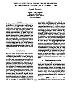
Admissible Cone Figure 1: The “admissible cone”, a topological cone denoted Wa , is the set of body translations which guarantee that, regardless of body rotation, all feature points will be within the FOV.

a.1)

a.2)

b.1)

b.2)

c.1)

c.2)

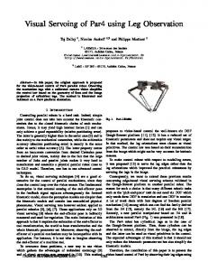
Figure 2: Simulation of three different artificial potential functions: a) the proposed NF in (7); b) the image-based potential function in (9), which leads to self occlusion and never reaches the goal; c) image-based potential function in (10) that accounts for self occlusion obstacles, nevertheless the potential function stops on a local minimum.

convergence is robust with respect to the model parameters of the camera and rigid body being servoed. Despite its advantages, there are many weaknesses to this approach. First, it is quasi-static, ignoring the mechanical system dynamics which impose restrictions on the speed of operation. As vision systems and processing get faster, such restrictions become undesirable. Second, there usually exist spurious critical points introduced by the alignment of y − y ∗ with the null space of J(q)T , and the absence of such spurious critical points is, to our knowledge, only guaranteed for a few cases [1, 4, 13]. Finally, there are many geometric problems associated with visual servoing such as losing sight of features due to (i) self occlusions or (ii) leaving the camera finite field-of-view (FOV). Usually these problems are ignored in analysis, and when encountered in practice simply cause the system to move into an emergency stop state, necessitating human intervention.

deals analytically with obstacle (i), though Malis and Chaumette anecdotally claim that self-occlusions never occur with coplanar feature sets, and they introduce an “adaptive” controller to keep one point of the body within the FOV, as detailed in [7].

Relation to Existing Literature: Recently, Malis and Chaumette [8, 9] used the homography between corresponding images – the current view and the desired view of a body – to partially reconstruct the pose up to a scaling in depth, for which they coined the term “2 21 D Visual Servoing” since it is neither fully image based nor fully reconstructive. Taylor and Ostrowski [12] present a similar quasi-global, quasi-static approach which uses the epipolar geometry to do a partial pose reconstruction, though their approach normalizes the translational component to unit length. Both of these works analytically demonstrate the robustness to camera parametric uncertainty, and Malis et. al. further validate the idea with an implementation for a 6DOF servoing system. These are two of the most novel approaches to date for 6DOF rigid body visual servoing and deserve careful attention. However, both of these approaches presuppose the quasi-static limitations of the classical image-based approach, and neither

Following that general approach, we first examine a topological model space for “occlusion-free” servoing, and then design a navigation function for that topology (Section 2). Of course the topological model is not enough; we need a coordinate system in which to do control, so in Section 2.3 we present a Cartesian coordinate system for our navigation function. Our simulations in Section 3 show the advantages of our algorithm over the traditional approach to visual servoing. We conclude with a brief account of the prospects for a family of image-based navigation functions.

Along different lines, Zhang and Ostrowski presented a dynamical visual servoing algorithm for a blimp for which they found a local diffeomorphism to the image plane to control 3DOF of the blimps motion [13], namely the radius and centroid (ρ, x, y) of an ellipse from a projected sphere. Contributions and Organization: The notion of an navigation function (NF) first articulated in [6], and briefly reviewed here in the appendix, proved fruitful for planar (3DOF) visual servoing [1], and this paper presents our recent efforts to design NF’s for spatial (6DOF) rigid body visual servoing.

2 NFs for Occlusion Free Servoing To use NF’s, we begin with a topological characterization of “occlusion-free” servoing (2.1), construct a NF for this model space (2.2), and then show how to “deform” it back to the problem at hand (2.3).

2.1 The Topology of Occlusion Free Servoing We must understand the topology of “occlusion-free servoing” in order to design a navigation function for it. Hence, we introduce the visible set of configurations, V, which render the feature points of the body completely in view of the camera – a simple and intuitive idea. In general, this set depends on the features chosen, the body geometry, the camera and the body’s configuration space.

We conveniently attach the body frame such that the (x, y)-plane contains the features, and the z-axis points toward the interior of the body. Letting R = [r1 , r2 , r3 ], we have © ª F = H ∈ SE(3) | TT r3 > 0 W = {H ∈ SE(3) | Hpi ∈ Wc , i = 1, . . . , N }

where Wc =

We will consider 2 cases: planar (n = 2) and spatial (n = 3) visual servoing. In both cases, we consider a world frame, F, whose origin is coincident with the camera pinhole and whose nth axis is orthogonal to the image plane. Also, we have a body fixed frame, FB . The body pose, H, is a homogeneous transformation matrix ½· ¾ ¸ R T n H ∈ SE(n) = | R ∈ SO(n), T ∈ R 0T 1 and any point with homogeneous coordinates p ∈ An , expressed with respect to FB , has coordinates Hp in F. We will assume that there is a goal pose H ∗ ∈ V. 2.1.1 Planar Case, V ⊂ SE(2): Suppose we have a convex polygonal rigid body in a plane, with N feature points on one edge, and let H ∈ SE(2) denote the pose of the body. For convenience we attach the x-axis of FB to the edge of the body as depicted in Figure 3. Denote the columns of R = [r1 , r2 ] and let © ª F = H ∈ SE(2) | TT r2 > 0 denote the set of configurations which are “facing” the camera pinhole. Similarly, let W = {H ∈ SE(2) | Hpi ∈ Wc , i = 1, . . . , N } denote the “workspace” of the camera, where © ª W c = p ∈ A 2 | p = o + α 0 v0 + α 1 v1 , α 1 , α 2 > 0

is the cone defined by the FOV, where o is the origin of F, and vi ∈ R2 are the vectors coincident with the FOV boundary and have a positive projection onto the y-axis of F. Clearly, V = F ∩ W ∈ SE(2) denotes all configurations for which the three features are projected to the image plane within the FOV and without self-occlusions. See Figure 3. We showed in [1] that for N = 3, V is equivalent to an open ball in R3 , which led to an image-based navigation function that rendered all of V as the domain of attraction for a goal H ∗. 2.1.2 Spatial Case, V ⊂ SE(3): We now consider a 6DOF rigid body with a set of N coplanar features. Just as in the planar case, H ∈ SE(3) represents the homogeneous transformation from FB to F.

(

3

p ∈ A |p = o +

i=3 X

αi vi , αi > 0, ∀i

i=0

)

is set of points on the interior of the FOV cone, defined by the four vectors vi , i = 1, . . . , 4. Finally, we have V = F ∩ W ∈ SE(3). Unfortunately, we have not yet characterized the topology of V, so we consider a subset V 0 ⊂ V which is slightly conservative with respect to the FOV. Assume all of the features are contained inside a circular disk of radius %, as depicted in Figure 1. We adopt the conservative requirement that center of the disk remain fully in the “admissible cone,”     0     i=3    0  X 3   Wa = p ∈ A | p =  α v , α > 0, ∀i + i i i %      i=0   1

The admissible cone is simply the set of locations in which all possible rotations of the body keep the features in the field of view. Hence ¾ ¸ ½ · R T 0 ∈ SE(3) | T ∈ Wa W = H= 0T 1 and V0 = W0 ∩ F

(1)

Proposition 1 The set V 0 ⊂ SE(3) is diffeomorphic to D5 × S 1 Proof.∗ The centroid is confined to move in a solid cylinder, i.e. R+ × D2 . Recall that the body coordinate frame, FB is attached such that the z-axis is orthogonal to the face (facing into the body) and the (x, y)-plane contains the feature points. Consider the fact that SO(3) is an SO(2) bundle over S2 , and identify the orientation of the z-axis with the basepoint in S2 . The requirement that the body faces the camera is a constraint on the the z-axis, namely that it always has a positive projection of onto the line-of-site. This yields a hemisphere; i.e. a diffeomorphic copy of D2 . An SO(2) bundle over D2 is diffeomorphic to SO(2) × D2 . Therefore V 0 ≈ R+ × D2 × SO(2) × D2 ≈ D5 × S1 . ∗ Robert Ghrist lent valuable insights into the topology of SO(n).

H∈F H∈ /W =⇒ H ∈ /V

PSfrag replacements

H∈ /F H∈W =⇒ H ∈ /V

H∈F H∈W =⇒ H ∈ V

xb yb xb

yb

yb

xb y1

y3 y2 y1

y2 y3

y1 y2 y3

Figure 3: A cartoon depiction of the sets F, W and V for a planar world. For convenience, the image plane is drawn in front of the camera pinhole. From left to right, the figures show three typical configurations of a rigid body with respect to a planar camera. Left: The edge is facing the camera, but the leftmost point is out of view. Center: Although completely within the camera workspace, the edge is facing away from the camera and is occluded by the body. Right: The edge is facing and within the field of view of the camera.

2.2 Navigation Function for D5 × S1 Let (x, θ) ∈ D5 × S1 , where† ¯ © ª D5 = x ∈ R5 ¯ kxk∞ < 1 Define

ϕ(x, e θ) = Proposition 2

kxk2 + 1 − cos(θ) Qi=5 2 i=1 (1 − xi )

ϕ=

ϕ e (1 + ϕ) e

(2)

Coordinate q1 q2 q3 q4 q5 q6

Valid Interval (0,∞) (−α,α) (−γ,γ) (−π/2,π/2) (−π/2,π/2) R mod 2π

Table 1: Coordinate bounds for h−1 (V 0 ) ⊆ R5 × S1 . The

(3)

is a navigation function on D5 × S1 with a minimum at (0, 0) and a saddle at (0, π), and achieves a maximum value of 1 on the entire boundary kxk∞ = 1 Proof. By design, ϕ achieves a maximum value of 1 on the entire boundary kxk∞ = 1. Furthermore, it is routine to verify that the two zeros gradient of ϕ are (0, 0) and (0, π), and that the Hessian at the critical points is nonsingular. Furthermore, the Hessian at (0, 0) is positive definite, hence it is a minimum, and it is indefinite at (0, π), hence it is a saddle. 2.3 Change of Coordinates Successful application of the NF presented above requires a change of coordinates from V 0 to D5 × S1 . We will find it convenient to introduce the specific set of coordinates, q ∈ Q, for SE(3) shown in Appendix B, and we will write matrices parameterized this way as h(q). † Note that the open disk is diffeomorphic to the cross product of open intervals.

parameters α and β are the horizontal and vertical FOV angles, respectively, i.e. cos α cos β = [0, 0, 1]vi /||vi ||.

The coordinates provide an intuitive handle on the topology of V 0 . Note that if we restrict the coordinates as in Table 1, we obtain a parameterization of V 0 . It is routine (though somewhat tedious) to find a closed form inverse, h−1 , for all points in V 0 . To deform V 0 into the simple model space in Section 2.2, we first map into local coordinates through h−1 . Then, we map the coordinate range in Table 1 through ÷ ! ¸T q1 − 1 q2 q3 q4 q5 , , , , b1 (q) = (4) , q6 q1 + 1 α γ π/2 π/2 so that b1 ◦ h−1 : V 0 → D5 × S1 . Finally, we “warp” the result to put the goal at the origin via b2 : D5 × S1 → D5 × S 1 ´   ³  ∗ a1 −a1

 1−a1 a1  .. b2 (a) =   ³ . ∗ ´ ∗

a5 −a5 1−a5 a∗ 5

     , a6 − a∗6   

a∗ = b1 ◦ h−1 (H ∗ ).

(5)

(6)

t = t1 > 0

t=0 PSfrag replacements

Initial Image Goal Image Image Plane Trajectories

t = t 2 > t1

t→∞

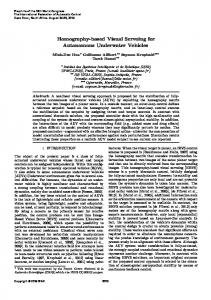
Figure 4: Simulation of visual servoing for a rigid body whose initial position is very close to the camera, but whose feature points are fully within the FOV. The navigation function proposed in Equation (7) correctly drives the body to the desired goal without violating the FOV constraints or self occluding. LEFT: The image plane trajectory of feature points. RIGHT: Snapshot at four successive times.

The result is a map b = b2 ◦ b1 ◦ h−1 : V 0 ≈ D5 × S1 and hence ϕ=ϕ◦b (7) is an NF on V 0 , with a unique global minimum H ∗ . A kinematic version of our controller is given in local coordinates by q˙ = −Dq (ϕ ◦ h)(q).

(8)

Figure 2 compares the performance of the potential function defined in (7) with that of (9). The left column represents visual illustrations of the body at various “snapshots” throughout its motion. The right column shows the trajectories of the four feature points. The black dots represent the initial feature locations and the white dots represent their goal locations. As expected, Figure 2(a) shows that (7) converges to the goal while all features points remain visible. However, the simulation of (9) in Figure 2(b) encounters a self-occlusion before convergences is obtained. A naive improvement accounting for obstacles, given by

3 Simulated Implementation Given the correspondence of image points, there are many algorithms for computing the pose of the body, H, and the goal, H ∗ . So, we define c : V 0 → Y ⊂ R2×N as the perspective projection of points HP . The feature points, P = [p1 , . . . , pN ], are expressed in body coordinates. Furthermore, there is always a unique inverse H = c−1 (y) for every point y ∈ c(V 0 ). The following simulations illustrate situations where naive approaches based on a simple measure of the distance of the image feature points to the goal fail, and how our algorithm overcomes the failures. It is assumed that there are four feature points (N = 4) on one face. Let ϕˆ be a continuous potential function defined on R2×4 by 4 X ϕ(y) ˆ := kyi − yi∗ k2 (9) i=1

where y ∗ = c(H ∗ ).

0

ϕ (y) :=

P4

∗ 2 i=1 kyi − yi k ¯ · ¸¯1/2 , ¯ ¯ Q ¯det yi yj yk ¯ {i,j,k}∈S ¯ 1 1 1 ¯

(10)

where S = {{1, 2, 3}, {1, 2, 4}, {1, 3, 4}, {2, 3, 4}}, was used for the simulations in Figure 2(c). In this case, there are no occlusions but the potential function stops on a local minimum. Figures 4 and 5, illustrate a situation where the body is very close to the image plane, but fully inside the (conservative) FOV, V 0 . Figure 5 reveals all the weaknesses of ϕ. ˆ The trajectory of one of the feature points clearly goes out the FOV (of course, we are able to allow the simulation to continue but an implementation would fail). Also, self-occlusion occurs, and the simulation stops on a local minimum. Figure 4, on the other hand, which has the same initial condition and goal, uses (7) and correctly executes the desired task as expected.

t = t1 > 0

t=0 PSfrag replacements

Initial Image Goal Image Image Plane Trajectories

t→∞

t = t 2 > t1

Figure 5: Simulation of visual servoing for a rigid body whose initial position is very close to the camera, but whose feature points are fully within the FOV. The potential function in Equation (9) is based only on image feature points and this trajectory goes out of the FOV, self occludes and ends in a local minima. LEFT: The image plane trajectory of feature points. RIGHT: Snapshot at four successive times.

Parametric Uncertainty: Of course c−1 depends on the intrinsic camera parameters (focal length, pixel size, etc.) and the body parameters, P , neither of which will be exactly known. To guarantee global convergence under (at least small) parametric uncertainty, we compute the goal pose, the current pose and the FOV cone all with respect to the same set of parameter estimates. We believe that modest perturbations of the parameters will not affect the convergence properties, though we have not calculated explicit bounds on the camera or body parameters which guarantee global convergence. However, our exploratory simulations suggest robustness to fairly large parametric uncertainty, and we are currently working on formal perturbation bounds to verify the robustness of our technique.

4 Conclusions

In this paper, we presented the first dynamical spatial rigid body visual servoing algorithm guaranteed to converge to a goal while avoiding self-occlusions and maintaining all feature points within in the field-ofview. This is achieved by a Navigation Function on a slightly conservative subset of the configurations in which all feature points are in view. Our approach requires reconstructing the current pose and the goal pose. It would be more desirable to avoid that reconstruction, or in the worst case, only partially reconstruct the pose. By designing an NF directly in image coordinates, this may be feasible.

Acknowledgements We thank Prof. Jorge Ambr´osio from Instituto Superior T´ecnico in Lisbon, Portugal for introducing the second author to the first and third as well as for several useful discussions concerning reconstruction of rigid body motion from camera feature data. Thanks to Prof. Robert Ghrist who lent valuable insights into the topology of SO(n).

A Review of Navigation Functions A review of NF’s follows.‡ An NF, ϕ, is a C 2 artificial potential function on a compact manifold, M , such that ϕ : M → [0, 1]. It must encode a goal set, G as the unique global minimum, ϕ(G) = 0, and achieve a maximum of 1 on the entire boundary of M , i.e. ϕ(∂M) = 1. Once constructed, one can obtain a second order controller which is guaranteed to converge to G for all points in M except a zero measure set, by simply following the negative gradient of the NF, and adding a suitable damping term [5]. As a simple example, consider a system with configuration space M = (−1, 1) whose dynamics are given by m¨ x=u and apply the NF ϕ(x) = x2 , and damping b. Letting k u = − Dx ϕ (x) − bx˙ 2 =⇒ m¨ x + bx˙ + kx = 0 ‡ For

a precise definition of Navigation Functions and their applications to robotics, see [11].

which renders 0 globally asymptotically stable, and is guaranteed to never hit the boundary set ∂M = {±1} for all initial positions on M .§ For the purposes of this paper, one may simply consider the first order gradient system given by x˙ = −Dx ϕ (x) when considering the convergence properties of the controller.

We will make frequent use of local coordinates for computation. Here we define a local chart h : Q → SE(3), where Q ⊂ R5 × S1 as follows. Let (11)

where h1 is a simple offset of the origin along the zaxis and h2 and h3 are parametrized by spherical coordinates and XYZ Euler-angles respectively as follows. Let · ¸ Ri (q) Ti (q) hi (q) = , i = 1, 2, 3. (12) 0T 1 For the translational component, we have T1 = [0, 0, %]T

R1 = I3×3

For the spherical coordinate component we have   sin q2 cos q3  sin q3 T2 (q) = q1  cos q2 cos q3

and



cos q2 0 R2 (q) =  − sin q2

− sin q2 sin q3 cos q3 − cos q2 sin q3

[2] Hoichi Hashimoto, Tsutomu Kimoto, Takumi Ebine, and Hidenori Kimura. Manipulator control with image-based visual servo. In International Conference on Robotics and Automation, volume 3, pages 2267– 2271. IEEE, 1991. [3] S. Hutchinson, G. D. Hager, and P. I. Corke. A tutorial on visual servo control. IEEE Transactions on Robotics and Automation, pages 651–670, October 1996.

B Local Coordinates

h = h 1 h2 h3 ;

References [1] Noah J. Cowan and Daniel E. Koditschek. Planar image based visual servoing as a navigation problem. In International Conference on Robotics and Automation, volume 1, pages 611–617, Detroit, MI, 1999. IEEE.

 sin q2 cos q3 . sin q3 cos q2 cos q3

Finally, for the Euler angles, we have T3 = 0 and   1 0 0 sin q4  R3 (q) =  0 cos q4 0 − sin q4 cos q4   cos q5 0 − sin q5  1 0 · 0 sin q5 0 cos q5   cos q6 sin q6 0 ·  − sin q6 cos q6 0  . 0 0 1 The coordinates are restricted as in Table 1.

§ To be precise, one must put bounds on the initial velocities to compute the domain of attraction on T M as a function of damping [5].

[4] D. Kim, A. A. Rizzi, G. D. Hager, and D. E. Koditschek. A “robust” convergent visual servoing system. In International Conf. on Intelligent Robots and Systems, Pittsburgh, PA, 1995. IEEE/RSJ. [5] D. E. Koditschek. The control of natural motion in mechanical systems. ASME Journal of Dynamic Systems, Measurement, and Control, 113(4):547–551, Dec 1991. [6] Daniel E. Koditschek and Elon Rimon. Robot navigation functions on manifolds with boundary. Advances in Applied Mathematics, 11:412–442, 1990. [7] Ezio Malis. Contributions a ` la mod´elisation et a ` la commande en asservissement visuel. PhD thesis, Universit´e de Rennes I, 1999. [8] Ezio Malis, Francois Chaumette, and Sylvie Boudet. Positioning a course-calibrated camera with respect to an unkown object by 2d 1/2 visual servoing. In IEEE Conf. on Robotics and Automation, 1998. [9] Ezio Malis, Francois Chaumette, and Sylvie Boudet. 2-1/2-d visual servoing. IEEE Transactions on Robotics and Automation, 1999. [10] Long Quan and Zhongdan Lan. Linear n-point camera pose determination. IEEE Transactions on Pattern Analysis and Machine Intelligence, 21(8):774–780, August 1999. [11] Elon Rimon and D. E. Koditschek. Exact robot navigation using artificial potential fields. IEEE Transactions on Robotics and Automation, 8(5):501–518, Oct 1992. [12] Camillo J. Taylor and James P. Ostrowski. Robust visual servoing based on relative orientation. In International Conf. on Robotics and Automation, 1998. [13] Hong Zhang and James P. Ostrowski. Visual servoing with dynamics: Control of an unmanned blimp. In International Conf. on Robotics and Automation, 1999.