Piecewise approximate implicitization: Experiments using industrial data Mohamed F. Shalaby1 , Jan B. Thomassen2,3, Elmar M. Wurm1 , Tor Dokken2 and Bert J¨ uttler1 1
2
3
Institute of Applied Geometry, Johannes Kepler University, Altenberger Str. 69, 4040 Linz, Austria; www.ag.jku.at, Email:
[email protected] SINTEF ICT, P.O. Box 124 Blindern, N–O314 Oslo, Norway; www.math.sintef.no, Email: [Jan.B.Thomassen|Tor.Dokken]@sintef.no Center of Mathematics for Applications, P.O.Box 1053 Blindern, N–0316 Oslo, Norway; www.cma.uio.no, Email:
[email protected]
Summary. We compare several methods for approximate implicitization by piecewise polynomials which have been developed by the authors, and a linear-algebrabased numerical method for implicitization which is provided as a part of MAPLE. We investigate both quantitative criteria (such as computing time, memory use, and the error of the approximation) and qualitative criteria. As demonstrated by the results, piecewise approximate implicitization is able to handle surfaces arising in industrial applications. However, special care has to be taken to avoid additional branches and unwanted singularities.
1 Introduction Parametric representations, such as NURBS surfaces, are used in most CAD systems see [Far02]. The parametric representation offers a number of advantages, e.g., simple techniques for display and for analyzing the geometric properties. On the other hand, implicitly defined surfaces are better suited in many applications, such as surface fitting (possibly subject to shape constraints, such as convexity) and the possibility of defining solids. In many applications, such as the computation of intersection and the detection of possible self–intersections, it is advantageous to combine both types of representations [Lee99, Tho05]. In order to exploit the potential of implicit representation, methods for conversion to and from implicit form are needed. The process of implicitization has been discussed by several authors. Various exact methods, such as resultants, Groebner bases, moving curves and surfaces exist [Cox97, Cox98, Cox99, Elk04, Hof93, Sed95, Veg97]. More recently, a number of approximate methods [Chu89, Dok01, Dok03, J¨ ut03] have emerged. They form a valuable alternative to the exact techniques.
2
M. Shalaby et al.
Several computational techniques for approximate implicitization of surfaces by a single algebraic surface have been compared in [Wur05]. However, for more complicated input surfaces, the approximation by a single algebraic surface is no longer feasible. In these cases, surfaces of relatively high degree would be needed, which may not be of much use for applications. In addition, the use of such surfaces would lead to numerical problems. Consequently, the use of piecewise polynomial representations (i.e., splines) is more appropriate. This paper presents a feasibility study for two methods for approximate implicitization by piecewise polynomials. The two methods are the scattered data fitting method developed at Linz (‘PPL’) , and the sampling-based method developed at SINTEF (‘PPS’). We restrict ourselves to the approximate implicitization of surfaces, since this case is more important for applications. Our results are based on work we have done in connection with the EU project GAIA II. The feasibility study is performed by applying the algorithms to two sets of “academic” and industrial test surfaces. The “academic” surfaces were constructed in the course of testing and developing the algorithms, while the industrial surfaces were supplied by the CAD vendor think3, which is a partner in the GAIA II project. We follow a procedure similar to [Wur05], where benchmarking for implicitization by polynomials has been presented. The input was a single parametric patch while the output was a single polynomial implicit function. In this paper, we have generalized this to the case of piecewise polynomials. Consequently, we can now deal with much more complicated surfaces. The approach enables piecewise surfaces – i.e., NURBS surfaces – as input, and piecewise polynomial implicit functions as output. In addition to studying the feasibility, the two methods are qualitatively compared to each other. Some of the test surfaces are given in terms of a single polynomial patch, and for this data it is possible to apply the implicitize routine implemented in MAPLE (‘ML’) and the previously studied single polynomial implicitization algorithm from SINTEF (‘PS’) [Wur05]. For these test cases we have been able to compare all four methods (PPL, PPS, ML, PS), and thereby study the effects of using implicit functions that are piecewise polynomial. This paper is organized as follows. Section 2 gives a short outline of the four methods of implicitization. Section 3 describes the test surfaces we have used in our experiments. In section 4, we comment on the parameters we are measuring in our experiments – time, memory usage, and approximation error – and specify how we made the measurements. The results are presented in section 5. In section 6 we give a qualitative analysis, and finally, in Section 7, we give a conclusion.
Piecewise approximate implicitization
3
2 The methods In this Section, we describe the four methods used for approximate implicitization. Only the first two of them (PPL and PPS) are relevant for piecewise implicitization. The two additional methods (PS and ML) are included in order to study some effects of using piecewise polynomials instead of just a single polynomial. All methods produce an approximate implicit representation of the form X f (x, y, z) = φj (x, y, z)cj (1) j∈J
with certain coefficients cj ∈ R and finite index set J . In the case of PPL and PPS, the basis functions φj (x, y, z) are trivariate tensor-product B-splines. Consequently, the output is a three–dimensional array of B-spline coefficients, along with three knot vectors. In the case of PPL, the array is sparse, and dynamical data structures may therefore be used in order to exploit the sparsity. PS and ML use a suitable basis of trivariate polynomials, such as Bernstein polynomials on a tetrahedron or tensor-product Bernstein polynomials. Note that none of these methods takes care of approximating the boundary curves (e.g., by clipping surfaces). This may be a subject of further research. Also, the use of hierarchical spline spaces (such as T-splines) should lead to a further improvement of the method. 2.1 PPL This method for approximate implicitization by piecewise polynomials has been developed at Linz [J¨ ut02]. It is characterized by the simultaneous approximation of sampled point data pi = (xi , yi , zi ), i ∈ I, and estimated unit normals ni at these points. If no other information is available (e.g., from a given parametric or procedural description of the surface, then each normal vector ni is estimated from the nearest neighbors of the point pi = (xi , yi , zi ). In addition, a regiongrowing-type algorithm is used for adjusting the orientation of the normal vectors. In order to control the shape of the resulting surface, an additional tension term is optimized. It pulls the approximating surface towards a simpler shape. A possible quadratic tension term is ZZZ 2 2 2 2 2 2 + 2 fxz + 2 fyz + fzz dx dy dz. (2) T (c) = fxx + 2 fxy + fyy Ω
By increasing the influence of this tension term, the resulting surface becomes more similar to a plane. The implicit function is obtained as the minimum of a convex quadratic objective function
4
M. Shalaby et al.
X
f (xi , yi , zi )2 + w||∇f (xi , yi , zi ) − ni ||2 + “tension”,
(3)
i∈I
where w is a positive weight. The weight controls the influence of the estimated normal vectors ni to the resulting surface. As observed in our experiments, increasing the weight can be used to ‘push away’ unwanted branches of the surface. This method is fully general, i.e., it can be applied to any space of functions, not only to piecewise polynomials. For practical applications, however, fast evaluation of basis functions is important. For this reason we implemented the algorithm for trivariate tensor-product B-splines. In this case, the basis functions ensure global smoothness, and the resulting system of linear equations is sparse. The domain of interest is divided into cubes of the same size. This is done by specifying a cell-size. In order to guarantee an integer number of cells, the bounding box of the input surface is enlarged a bit. We consider only the cubes which contain data, and its neighbors. We named it as “active cells”. The domain of the spline functions consists only of the active cells. Another input parameter is the degree d of the spline function. We choose the knot vector with simple knots in the interior, so the continuity is C d−1 . The choice of the degree d depends on the singularities of the given curve/surface. Singularities can be reproduced by the algebraic approximation, provided that a sufficiently high degree is employed in the algebraic approximation. For example, in 2D, in order to represent a double point, one has to use degree three or higher. See also the discussion in Section 6.2, which addresses the conflict between pushing away unwanted branches and avoiding singularities. Due to the compact support of the B-splines, the implementation is relatively fast because of the sparsity of the resulting linear system of equations. Consequently, even complicated singular surfaces can be implicitized. In this case, it is an important issue to create a consistent orientation of the (estimated) normals ni , and this can be achieved by a propagation technique [J¨ ut03]: First, an initial approximation is computed using only information from one part of the data, where a consistent orientation could be created without ambiguities. The result is then used to propagate the orientation of the normals to the neighboring segments of the data. The details of this ˇ method are described in [J¨ ut02, Wur05, Sir05]. A fast implementation of the method is important, since is then feasible to iterate this process, for orientation propagation and for adjusting the estimated normals. 2.2 PPS The piecewise polynomial approximate implicitization algorithm made at SINTEF is a generalization of the polynomial SINTEF algorithm from [Dok03, Wur05]. Essentially, it is a generalization in two ways: First, it produces a piecewise polynomial implicit function, more specifically a trivariate tensor
Piecewise approximate implicitization
5
product B-spline function. The three knot vectors of the B-spline function are obtained by dividing the bounding box of the input surface into n × n × n cells, where n is a user-defined integer, and adding d additional knots at the boundaries (where d is the degree d of the spline function). This gives interpolating boundary conditions. The knot vector is chosen with simple knots in the interior, hence the continuity equals C d−1 . The second generalization is the use of point sampling on the input surface. Thus a linear system of equations is set up such that each point defines a row in the matrix of the equation, X f (xi , yi , zi ) = φj (xi , yi , zi )cj = 0, i ∈ I. (4) j∈J
Points are sampled according to a uniform grid in the parameter domain. The density of the points in the parameter domain is chosen large enough such that the matrix equation is over-determined. From experimenting with the algorithm, a good choice for the number of points in the algorithm was found to be roughly two times the number of coefficients in the implicit function. Thus, if M × N denotes the dimensions of the matrix Φij = φj (xi , yi , zi ), we have M ≈ 2N . The rest of the algorithm proceeds essentially in the same way as the polynomial version [Dok03, Wur05]: We get a matrix, and we want to find a suitable vector in an approximate null space of this matrix. This is done by SVD, and the resulting approximate nullvector will be the vector of coefficients for the implicit spline function. Special care must be taken to ignore vectors belonging to singular values that are exactly zero. Such singular values appear in general because some cells in the rectangular space grid are outside the support of the relevant basis functions, and this produces columns of zeros in the matrix. We remove these columns before we run the SVD. We also take the square of the matrix Φ, i.e. we use ΦT Φ, which further reduces the size of the matrix from M × N to N × N before SVD is applied. The coefficients corresponding to the original zero columns are subsequently arbitrarily set to zero. The input parameters to this algorithm, in addition to the surface, are the degree of the spline approximation and the number of grid cells in each direction. 2.3 PS This method is the single polynomial approximate implicitization method developed at SINTEF, which is also based on singular value decomposition (SVD). A description can be found in [Dok03]. In brief, we insert the parametric surface into an implicit polynomial function of chosen degree and with unknown coefficients. This results in the factorization
6
M. Shalaby et al.
f (x(u, v)) = Φ(u, v)T D c,
(5)
where Φ is a vector of basis functions (bivariate tensor-product Bernstein polynomials) and c contains the unknown coefficients of f . In addition, it contains a certain matrix D, which depends on the given surface. The coefficients of the implicit representation are then found as the eigenvector corresponding to the smallest singular value of that matrix. The only input parameter is the degree of the implicit function. For this we have either used the exact degree, or, if the exact degree is too high, a relatively low degree to produce an approximation. We have found d = 5 to be a good choice. 2.4 ML The ‘implicitize’ routine in MAPLE is based on the algorithm described in [Cor00], which relies on numerical linear algebra. Again, the parametric surface is inserted into an implicit function of a chosen degree and unknown coefficients. The implicit approximation then is found by minimizing the integral of the resulting parametric function over the given parametric domain, with respect to the unknown coefficients. The eigenvector associated with the smallest eigenvalue of a certain matrix has to be computed. In order to generate this matrix, several integrations have to be performed.
3 Test cases Piecewise approximate implicitization methods work for both curves and surfaces. In the sequel we consider only the surface case, since it is more interesting for applications, and – unlike curves – many surfaces are not accessible for exact implicitization techniques. The test cases used in benchmarking the algorithms can be divided in two groups. The first group contains “academic” examples, which were constructed at SINTEF and Linz in order to help developing the algorithms and to display essential features like singularities and self-intersections in a relatively simple setting. The second group consists of industrial examples, provided by CAD vendor think3 (a partner in the GAIA II project). The surfaces are visualized and described in Fig. 1 and Fig. 2. The tables in these figures give a short description of the various test cases, along with short motivations for choosing these examples. The industrial surfaces have been generated using geometrical operations such as sweeping, which may create severe problems with self-intersections. Some of these example have already been used in [Wur05]. In this paper, we focus on the more complicated industrial examples, which could not be dealt with previously.
Piecewise approximate implicitization
Looped patch
Surface 7x7
Nested surface
nodal
Quartic surface
Surface 6x5
Surface Looped patch
Degree Description (3, 1) Self-intersecting. It is the simplest type of surface with this property. Nested nodal (3, 3) Doubly self-intersecting. The bi-degree of the surface B´ezier representation suggests an exact implicit representation of degree 2 × 3 × 3 = 18, but due to reflection symmetries the correct degree is 6. Quartic surface (3, 2) Surface with self-intersection curves and a cusplike singular point. As with the ‘nested nodal surface’ the correct implicit degree is reduced, in this case to 4. Surface 7x7 (7, 7) High degree oscillating patch without singularities. The theoretical algebraic degree of this surface is 2 × 7 × 7 = 98. Surface 6x5 (6, 5) Self-intersecting patch. A self-intersecting curve is moved in space and at the same time bent. The theoretical algebraic degree of this surface is 2 × 6 × 5 = 60.
Fig. 1. Academic test surfaces
7
8
M. Shalaby et al.
Self ucurves
Self pipe Surface Self ucurves
Simplesweep
Self sweep
Self pipe
Self proport
Simplesweep
Self sweep
Self proport
Degree Description (4, 2) Surface with a closed self-intersection curve. Two points on this curve are cusp-like singularities. Effectively, the degree of the exact implicit representation for this surface is 8. The surface is obtained by blending a curve segment with a node between two non-self-intersecting curves. (4, 3) Self-intersecting. The exact implicit representation has degree 6. The surface is obtained by “sweeping” between a piece of a node and a piece of a parabola. (12, 1) The surface is generated by sweeping a line with constant draft angle along a planar curve. It consists of 8 patches each of degree (12, 1) connected with C 2 continuity. (3, 3) The surface is generated by sweeping a circular section along a curve. It consists of 2310 bicubic patches connected with C 2 continuity. (3, 3) The surface is a general sweeping surface. It is obtained by sweeping a curve (drive) along another curve (boundary). It consists of 1824 bicubic patches connected with C 2 continuity.
Fig. 2. Industrial test surfaces (data courtesy of think3)
Piecewise approximate implicitization
9
4 Quantitative criteria The three main criteria for the comparison are the computing time, the memory needed by the algorithms being tested, and errors measured for the resulting implicit surface. The quoted time is an approximation of the processor time used by the program, and similarly for the memory. These quantities, in the case of PPL, PPS and PS, were measured with standard Linux tools (time and top). In the case of ML the ‘profile’ procedure of MAPLE was used. For the error measurements, we consider a set of points pi on the parametric surface and compute their Euclidean distances with respect to the implicit surface, using a Newton-like iteration procedure. In order to get a scale independent measurement, we divide this by the length L of the shortest side of the bounding box of the parameterized surface. In a nutshell, the value listed for the error is a scaled version of the average Euclidean distances of the sampled points pi from the implicit surface. The computation via footpoint computation is conservative, hence it will overestimate the real error. Clearly, the average footpoint distance does not reflect the reproduction of singularities. A suitable error measure for singularities, which seems to be currently unknown, would therefore be interesting. All tests were performed on standard hardware. Both PPL and ML were run on a computer with an Intel(R) Xeon(TM) CPU 2.40GHz, while the PPS and PS were tested on an Intel Pentium IV 2.80 GHz processor. Both systems had (approximately) the same operating system (Linux) and working memory. According to the CPU benchmark tests [Hav05], both systems have almost the same performance.
5 Results For implicitizing multi-patch parametric surfaces, the two piecewise approximate implicitization methods that are relevant are PPL and PPS. Even in the case of single patch parametric surfaces, which can be handled with single polynomial methods (ML, PL), these piecewise methods are able to produce an algebraic representation of lower degree. Both the PPL and PPS take as input the degree of the B-spline and information about the number of cells in the input data bounding box. In the case of PPL, the cell size is specified and the input data bounding box is enlarged a bit in order to fit an integer number of cubic cells. In the case of PPS, the input data bounding box is subdivided into n3 cells, where n is a user-defined integer. The results given in Tables 1 were computed using cubic B-splines. For both algorithms, almost the same “total” number of cells were used. However, as described in Section 3, PPL considers only the “active cells”. Their number
10
M. Shalaby et al.
Example (#Points for PPL)
Degree PPL for # Active Time Error # Cells PPL&PPS Cells Memory Looped patch 3 84 3.72 sec. 0.000168 216 (2250) 18.41 MB Nested nodal surface 3 101 6.96 sec. 0.005170 216 (2500) 17.90 MB Quartic surface 3 168 5.52 sec. 0.000455 216 (2500) 31.32 MB Surface 7x7 3 93 4.70 sec. 0.000235 216 (2500) 24.40 MB Surface 6x5 3 111 4.35 sec. 0.000572 216 (2500) 12.44 MB Self ucurves 3 154 4.77 sec. 0.000210 216 (2500) 30.70 MB Simplesweep 3 178 5.91 sec. 0.000026 216 (2500) 38.02 MB Self sweep 3 168 6.34 sec. 0.002690 216 (2500) 36.57 MB Self pipe 3 174 5.28 sec. 0.002740 216 (2500) 30.64 MB Self proport 3 172 6.29 sec. 0.004991 216 (2500) 37.68 MB
PPS Time Memory 9.7 sec. 11 MB 6.9 sec. 5.2 MB 10 sec. 9.3 MB 9.9 sec. 12 MB 8.7 sec. 8.5 MB 7.8 sec. 8.6 MB 12 sec. 13 MB 13.3 sec. 14 MB 16.7 sec. 17 MB 16.9 sec. 16 MB
Degree for ML&PS 0.02 3
Error
0.029
6
0.003
4
0.008
5
0.013
5
0.01
8
0.008
6
0.025
ML PS Time Time Error Memory Memory 4.64 sec. ∼0 ∼0 11.75 MB 0.9 MB 48.76 sec. 0.16 sec. ∼ 0 45.79 MB 1.3 MB 9.64 sec. 0.01 sec. ∼ 0 15.31 MB 0.9 MB failed 0.6 sec. 0.0249 1.5 MB 126.99 sec. 0.2 sec. 0.0161 30.35 MB 1.3 MB 206.99 sec. 1.38 sec. ∼ 0 129.95 MB 1.8 MB 30.14 sec. 0.25 sec. ∼ 0 47.98 MB 1.2 MB failed failed
0.055
failed
failed
0.035
failed
failed
Table 1. Result for the academic (upper part) and industrial (lower part) surfaces.
Piecewise approximate implicitization
11
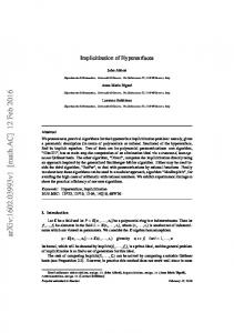
is listed separately in the table. For PPL we list also the number of sampled points for each test case. The results of PPL and PPS , see table 1, show that piecewise approximate implicitization is feasible. For all test cases, a tensor B–spline of degree (3×3× 3) are used. For both algorithms, the implicitization is performed in reasonable time, with reasonable memory usage, and with relatively small error. There are some small differences between the algorithms. The results of ML and PS are also shown in the same table. Both methods take a parametric surface in terms of a single polynomial patch and a chosen degree of the implicit representation as input. Hence some analysis of the problem is required prior to performing an implicitization. The methods may fail if the chosen degree was too low/high compared with the exact one. The first three academic test cases and the first two industrial cases in table 1 were computed using the exact algebraic degree. In this case, PS computes the exact implicit equation. ML, using the ‘numerical’ option, was able to compute an approximation within tolerances. For the test cases Surface 7x7 and Surface 6x5 the exact algebraic degrees are too high. We computed these two examples using degree 5, for PS & ML, as the degree of the implicit representation. ML, in the case of Surface 7x7, failed to give an implicit representation due to the low degree specified. Both methods, PS & ML cannot handle multi-patch parametric surfaces, and they therefore fail to compute the last three test cases in table 1. In order to demonstrate the feasibility of the methods, we plot the implicit surface for two selected test cases: Quartic surface and Self pipe, see Fig. 3. PPL is able to generate surfaces without additional branches (cf. Fig. 3 ).
6 Qualitative comparisons Finally we discuss some properties of the four techniques. Since pushing away unwanted branches is the most important issue, we dedicate a separate subsection to this subject. 6.1 General criteria • Both PPL and PPS are able to handle general surfaces. Consequently, they can also be used to implicitize procedurally defined surfaces, since they only need samples of points. In contrast, PS and ML can be applied only to parametrically defined rational surfaces (patches of NURBS). • Both PPL and PPS are able to compute an approximate implicitization for all test cases with reasonable error. • In the case of one-patch parametric surfaces, PS (and similarly PPS) is able to reproduce the exact implicitization (within tolerances) if the exact degree is chosen. ML reproduces the exact implicitization if the symbolic
12
M. Shalaby et al.
Quartic surface (PPL)
Self pipe(PPL)
Quartic surface (PPS)
Cut–away view Self pipe (PPL)
of
Self pipe (PPS)
Fig. 3. Results (PPL, PPS)
integration option is used. Using this option the computation is extremely slow. For our test cases, we used the numerical option. PPL does not reproduce the exact implicit representation, since it approximates not only the points, but also the estimated unit normals. • In the case of spline surfaces, the notion of an exact implicitization does not make much sense. In the case of one-patch parametric surface, PS is the fastest and the most accurate method. • For both PPL and PPS one may increase the number of segments and use a low degree, while maintaining the same level of accuracy. A trivariate tensor-product spline function with k inner knots in each direction has (k + 1)3 cells/segments and (k + d + 1)3 scalar coefficients. In practice, however, it is more important how many of the cells are aligned with the surface (‘active cells’), and the number of degrees of freedom will be more in the order of (k + d + 1)2 (but depends on the geometry of the surface).
Piecewise approximate implicitization
13
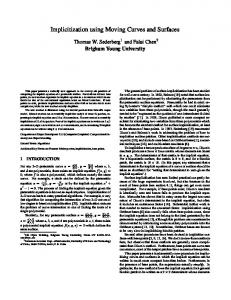
• All methods need the degree as an input parameter. In addition, both PPL and PPS need information about the number (or size) of the cells. • Currently, PPL is faster and more accurate than PPS for all test cases. • In order to implicitize with piecewise polynomials, it is necessary to regularize the problem, since cells without or with only a small number of data may cause numerical problems. In the case of PPL, this was achieved by introducing an additional tension term. It is possible to develop (semi–) automatic techniques for adjusting the influence of this term. 6.2 Avoiding unwanted branches and the reproduction of singularities All methods may produce unwanted branches of the surfaces, and possible additional singularities. The latter ones can be detected by analyzing the singular points of the implicitly defined surface, along the parametric surface. If one of these singular points corresponds to only one point on the parametric surface, which is not singularly parameterized, then it is an additional singularity, which was produced by the implicitization process. PPL provides two possibilities for pushing away these branches away from the desired part of the surface. First, they can be avoided by exploiting the simultaneous approximation of points sampled from the surface and the associated unit normals. By increasing the number of sampled points and/or the weight w in the objective function, the result of the approximation can be modified so as to become more similar to the signed distance function of the surface. Second, the tension term (3) can be used to avoid these unwanted branches. However, this term tends to flatten the implicitly defined surface, and it may therefore lead to poorer approximations. It is hoped that an improved version of PPS can achieve similar effects by taking the results for more than one singular value into account. This is subject of on–going research. The two goals of reproducing singularities and avoiding unwanted branches are often in conflict with each other. This is illustrated by Fig. 4, which shows two approximate implicitizations of the ‘nested nodal surface’. The piecewise polynomial approximation (left) has no unwanted branches, but the reproduction of the singularity is rather poor. On the other hand, the implicitization by a single high degree polynomial produces many unwanted branches, but it reproduces the double lines very well.
7 Conclusion We have compared several algorithms for approximate implicitization by polynomials and by piecewise polynomials. As demonstrated by the results, industrial data needs piecewise polynomials, in order to generate well–defined
14
M. Shalaby et al.
Fig. 4. Reproducing singularities vs. avoiding unwanted branches.
implicit representations of low degree. It was shown that approximate implicitization of real–world surfaces is possible in reasonable time on standard hardware. Further research will focus on the important issue of avoiding unwanted branches and additional singularities. Acknowledgment. This research has been supported by the European Commission through project IST-2001-35512 ‘Intersection algorithms for geometry based IT-applications using approximate algebraic methods’ (GAIA II).
References [Chu89] [Cor00]
[Cox97] [Cox98] [Cox99]
[Dok01] [Dok03]
[Dok05] [Elk04]
Chuang, J., Hoffmann, C.: On local implicit approximation and it’s applications. ACM Trans. Graphics 8, 4:298–324, (1989) Corless, R., Giesbrecht, M., Kotsireas, I., Watt., S.: Numerical implicitization of parametric hypersurfaces with linear algebra. In: AISC’2000 Proceedings, Springer, LNAI 1930. Cox, D., Little, J., O’Shea, D.: Ideals, Varieties and Algorithms, Springer, New York 1997. Cox, D., Little, J., O’Shea, D,: Using algebraic geometry, Springer Verlag, New York 1998. Cox, D., Goldman, R., Zhang, M.: On the validity of implicitization by moving quadrics for rational surfaces with no base points, J. Symbolic Computation, 11, (1999) Dokken, T.: Approximate Implicitization, in: Lyche, T., Schumaker, L. (eds.), Mathematical methods in CAGD, Nashboro Press, 2001, 1-25. T. Dokken and J. Thomassen, Overview of Approximate Implicitization, in: Topics in Algebraic Geometry and Geometric Modeling, AMS Cont. Math. 334 (2003), 169–184. Dokken, T., Thomassen, J.: Weak approximate implicitization, submitted to these proceedings. Elkadi M., Mourrain B.: Residue and Implicitization Problem for Rational Surfaces, Applicable Algebra in Engineering, Communication and Computing, (2004), 361-379.
Piecewise approximate implicitization [Far02] [Hav05] [Hof93] [J¨ ut02] [J¨ ut03]
[Lee99] [Tho05]
[Sed95] ˇ [Sir05] [Veg97]
[Wur05]
15
Farin, G.: Curves and Surfaces for Computer Aided Geometric Design, Academic Press, 2002. PoVRAY Benchmarks, http://new.haveland.com/povbench/graph.php Hoffmann, C.: Implicit Curves and Surfaces in CAGD, Comp. Graphics and Applics. 13:79–88, (1993) J¨ uttler, B., Felis, A.: Least-squares fitting of algebraic spline surfaces, Advances in Computational Mathematics 17:135–152, (2002) J¨ uttler, B., Wurm, E.: Approximate implicitization via curve fitting, in L. Kobbelt, P. Schr¨ oder, H. Hoppe (eds.), Symposium on Geometry Processing, Eurographics / ACM Siggraph, New York 2003, 240-247. Lee, K.W.: Principles of CAD/CAM/CAE Systems, Prentice Hall, 1999. Thomassen, J., Self-intersection problems and approximate implicitization, in: Dokken, T., J¨ uttler, B. (eds.), Computational Methods for Algebraic Spline Surfaces, Springer, Berlin 2005, 155-170. Sederberg, T., Chen F.: Implicitization using moving curves and surfaces. Siggraph 1995, 29:301–308, (1995) ˇır, Z.: Fitting of Piecewise Polynomial Implicit Surfaces, Proc. of the S´ 24rd Conference on Geometry and Computer Graphics, Ostrava, in press. Gonzalez-Vega, L.: Implicitization of parametric curves and surfaces by using multidimensional Newton formulae. J. Symb. Comput. 23(2-3), 137151 (1997) Wurm, E., Thomassen, J., J¨ uttler, B., Dokken, T.: Comparative Benchmarking of Methods for Approximate Implicitization, in: Neamtu, M., and Lucian, M. (eds.), Geometric Design and Computing, Nashboro Press, in press.