Dec 28, 1999 - 7 Dynamically Coloured Petri Nets into Piecewise Deterministic Markov ...... D1 There are no explosions, i.e. the time at which a token colour ...
NLR-TP-2000-428
Piecewise Deterministic Markov Processes represented by Dynamically Coloured Petri Nets Revised edition M.H.C. Everdij and H.A.P. Blom
Nationaal Lucht- en Ruimtevaartlaboratorium National Aerospace Laboratory NLR
NLR-TP-2000-428
Piecewise Deterministic Markov Processes represented by Dynamically Coloured Petri Nets Revised edition M.H.C. Everdij and H.A.P. Blom
This research has been carried out under NLR's basic research programme, Work Plan number L.1.B.2. The contents of this report may be cited on condition that full credit is given to NLR and the authors.
Division:
Air Transport
Issued:
December 1999
Classification of title:
Unclassified
-2NLR-TP-2000-428
DOCUMENT CONTROL SHEET Report Title
Piecewise Deterministic Markov Processes represented by Dynamically Coloured Petri Nets
Version
0.3
Date
21-03-2003
Customer
NLR
Order No.
5091922
Project
DYNAMO
NLR division
Air Transport
Document change log Version Nr
Issue date
Details of changes
0.1
28-12-1999
IEEE anonymous peer review comments incorporated
0.2
15-09-2000
Review comments of NLR reviewer incorporated
0.3
21-03-2003
Technical update
Version 0.3 Authors
M.H.C. Everdij H.A.P. Blom
Internal reviewer
M.B. Klompstra
Signature
Date
-3NLR-TP-2000-428
Summary Piecewise Deterministic Markov Processes (PDPs) are known as the largest class of Markov processes virtually describing all continuous-time processes not involving diffusions. In general the state space of a PDP is of hybrid type, i.e. a tensor product of a discrete set and a continuous-valued space. Since Stochastic Petri Nets have proven to be extremely useful in developing continuous-time Markov Chain models for complex practical discrete-valued processes, there is a clear need for a type of Petri Nets that can play a similar role for developing PDP models for complex practical problems. To fulfil this need, the paper defines a new type of Petri Net, named Dynamically Coloured Petri Net (DCPN), and proves that there exist into-mappings between PDPs and DCPNs. This report version (dated 2003) is a slightly revised edition of a report (dated 2000) with the same title, authors and report number.
-4NLR-TP-2000-428
Contents 1
Introduction
8
2
Piecewise Deterministic Markov Processes
9
3
Main Petri Nets extensions
11
4
Dynamically Coloured Petri Nets
12
5
Example DCPN
15
6
Piecewise Deterministic Markov Processes into Dynamically Coloured Petri Nets
17
7
Dynamically Coloured Petri Nets into Piecewise Deterministic Markov Processes
20
8
Example PDP
23
9
Conclusions
24
10 References
24
1 Figure
Appendices
27
A
Formal definition of Dynamically Coloured Petri Nets
27
B
Characterisation of Q in terms of DCPN
30
(32 pages in total)
-5NLR-TP-2000-428
List of acronyms DCPN
Dynamically Coloured Petri Net
ECPN
Extended Coloured Petri Net
HLHPN
High-Level Hybrid Petri Net
PDP
Piecewise Deterministic Markov Process
PN
Petri Net
RG
Reachability Graph
RRG
Reduced Reachability Graph
List of symbols ∪θ
:
Unity
∩θ
:
Intersection
|·|
:
Number of elements in a set
IRn
:
n-dimensional rational numbers
IN
:
Natural numbers
∂E
:
Boundary of open subset E
R0 – R 4
:
Rules
D1 – D 3
:
Conditions
xt
:
Continuous state
θt
:
Discrete state
ξt
:
Hybrid state
Eθ
:
Open subset of IRd(θ)
E
:
Disjoint unity of all subsets Eθ
E
:
Borel-measurable subsets of E
Γ∗
:
Reachable boundary of E
K
:
Countable domain for process {θt }
d(·)
:
Function that maps K into IN
gθ (·)
:
Lipschitz continuous function
φθ,x0
:
Flow
λ(θt , xt )
:
Rate of Poisson point process
Gξ (·)
:
Survivor function
IA
:
Indicator function
Q(·; ξ)
:
Transition measure
-6NLR-TP-2000-428
t
:
Time
τ , τk
:
Stopping times
∆
:
Time
t∗ (θ, x)
:
Time until first boundary hit
t∞ (θ, x)
:
Explosion time of flow φθ,x (·)
σk , ζ k
:
Samples from probability distributions
Nt
:
Number of jumps until time t
P
:
Set of places
P(A)
:
The place that is connected to arc A
T
:
Set of transitions
TG
:
Set of guard transitions
TD
:
Set of delay transitions
TI
:
Set of immediate transitions
T (A)
:
The transition that is connected to arc A
A
:
Set of arcs
AO
:
Set of ordinary arcs
AE
:
Set of enabling arcs
AI
:
Set of inhibitor arcs
A(T )
:
Set of arcs connected to transition T
Ain (T )
:
Set of input arcs of transition T
Ain,O (T )
:
Set of ordinary input arcs of transition T
Ain,OE (T )
:
Set of input arcs of transition T that are either ordinary or enabling
Aout (T )
:
Set of output arcs of transition T
N
:
Node function
S
:
Set of colour types
C
:
Colour function
I
:
Initial marking
V
:
Set of token colour functions
VP
:
Token colour function for place P
G
:
Set of transition guards
GT
:
Transition guard for transition T
D
:
Set of transition delays
DT
:
Transition delay for transition T
-7NLR-TP-2000-428
F
:
Set of firing measures
FT
:
Firing measure for transition T
P , Pi
:
Place
P (A(T ))
:
Set of places connected to T by the set of arcs A(T )
T , Ti
:
Transition
TiG
:
Guard transition
TiD
:
Delay transition
A, Ai
:
Arc
C(P )ms
:
Set of all multisets over C(P )
c, ct
:
Colour of token or vector of colours
δT
:
Rate of transition delay
zt
:
Vector containing position and velocity of aircraft
vt
:
Velocity of aircraft
u
:
Random number
pB|C
:
Conditional probability density function
α`
:
Auxiliary variable
f
:
Vector of zeros and ones
ϑi , m i
:
Element of K
vi,t , vi
:
Number of tokens in place Pi
i
:
Nodes of reachability graph
xi,j,t
:
Colour of jth token in place Pi at time t
L
:
Set of paths characterised by labels
L
:
Set of transitions, element of L
V,V
-8NLR-TP-2000-428
1 Introduction The motivation for this research stems from the following unsolved issue in air traffic: under which conditions is it possible to reduce established criteria for separation between aircraft without sacrificing safety in the form of collision risk. Studying this issue is most urgent for those regions in the world where air traffic is most dense, and consequently where the interplay between aircraft and air traffic management centres is most complex. During an earlier study (Bakker and Blom, 1993) a clear relation has been established between collision risk and the evolution of the density of the joint states of two or more flying aircraft. During the subsequent search for Markov process models to characterise the evolution of such densities the class of Piecewise Deterministic Markov Processes (PDPs) was identified as a very useful one (Everdij et al., 1996). At this moment, this type of modelling and evaluation has been accomplished for several air traffic management situations (Blom et al., 1998). It appeared to be less straightforward to develop an appropriate PDP model for a process as complex as air traffic management. For this reason a Petri Net has been developed (Everdij et al., 1997) that supports the modelling of PDPs for complex practical problems, similarly as Stochastic Petri Nets support the development of a Markov Chain for discrete valued complex problems. This new Petri Net and its precise relation with PDPs form the subject of this paper. Davis (1984, 1993) has introduced PDPs as the most general class of continuous-time Markov processes which include both discrete and continuous processes, except diffusion. A PDP consists of two components: a discrete valued component and a continuous valued component. The discrete valued component models the mode process {θ t }. At discrete times, {θt } may switch to another mode value which is selected according to some probabilistic relation. The continuous valued component models the drift process {x t }, as a solution of a θt -dependent differential equation. At discrete moments in time, {x t } may jump according to some relation, which makes it only piecewise continuous. The PDP state is given by ξ t = Col{θt , xt }, and is called a hybrid state. A switch and/or a jump occurs either when a doubly stochastic Poisson process generates a point or when {x t } hits the boundary of a predefined area. If {x t } also makes a jump at a time when {θt } switches, this is said to be a hybrid jump. PDPs are defined such that their sample paths are right-continuous and have left-hand-side limits, often shortened as c`adl`ag, which is an acronym for the French ‘continu a` droite, limites a` gauche’, see e.g. Protter (1990). Branicky (1995) identified a close relation between PDPs and Hybrid Automata. The latter have been shown useful for application in problems of decidability, formal verification and control synthesis (Alur et al., 1993; Lygeros et al., 1998; van Schuppen, 1998; Sipser, 1997; Tomlin et al., 1998; Weinberg et al., 1996). An important limitation, however, is that Poisson type of events
-9NLR-TP-2000-428
of PDPs are not covered by Hybrid Automata, which makes them less effective in modelling stochastic effects than PDPs. A Petri Net representing a PDP should make direct use of the specific PDP structure in order to have an advantageous modelling power. The established Petri Net descriptions (see David and Alla (1994) for a good overview) appear not to have this property. The newly developed Dynamically Coloured Petri Net (DCPN) presented in this paper does. The values of the mode process can be mapped to the distribution of tokens among the places in the DCPN. As long as the tokens remain where they are, the mode keeps the same value. The continuous process values are directly coupled to the token colours but they are evaluated while the tokens reside in the places and not during the transport of tokens. These colours may however influence the mode switches, both in time and in value. In this way, the continuous valued processes and the discrete valued processes are coupled and decoupled at the same level as they are in Piecewise Deterministic Markov Processes. This makes that into-mappings between PDPs and DCPNs exist. The key result of this paper is the proof of the existence of these into-mappings. An issue that deserves special attention when relating PDPs to Petri Nets is that for PDP, at each moment in time, there is a unique realisation of the state, while a Petri Net may make a sequence of jumps at a single moment in time. The into-mappings between PDPs and DCPNs we develop in this paper take care of this issue. The organisation of this paper is as follows. First, in Section 2, Piecewise Deterministic Markov Processes are described briefly. Next, Section 3 discusses how the main Petri Nets extensions from literature relate to PDPs. Subsequently, Section 4 defines Dynamically Coloured Petri Nets. Section 5 presents a DCPN example for a practical situation. Section 6 shows that a PDP can be represented by a DCPN. Section 7 shows that a DCPN can be represented by a PDP. Section 8 gives an example PDP that models the same process as the one described by the example DCPN in Section 5. Finally, Section 9 draws conclusions.
2 Piecewise Deterministic Markov Processes A Piecewise Deterministic Markov Process is defined as follows (see Davis (1993)): For each θ in its countable domain K, let Eθ be an open subset1 of IRd(θ) , where d is a function that maps K into IN . For each θ ∈ K, consider the ordinary differential equation x˙ t = gθ (xt ), with x0 ∈ Eθ , where gθ : IRd(θ) → IRd(θ) is a locally Lipschitz continuous function. Given the initial value x 0 , this differential equation has a unique solution given by the flow φ θ,x0 . Suppose at some time instant τ the PDP state ξτ assumes value ξ = (θ, x) = (θ, φθ,x (0)). If no jumps occur, the 1
Note that Davis writes Eθ = Eθ0 ∪∂1 Eθ0 , with Eθ0 an open subset of IRd(θ) , and ∂1 Eθ0 those points on the boundary
of Eθ0 from which Eθ0 can be reached (by the flow φ), but which cannot be reached from the interior of Eθ0 .
- 10 NLR-TP-2000-428
process state at t ≥ τ is given by ξt = (θt , xt ) = (θ, φθ,x (t − τ )). At some moment in time, however, the process state value may jump. Such moment is generated by either one of the following events, depending on which event occurs first: 1. A Poisson point process with jump rate λ(θ t , xt ), t > τ generates a point. 2. The piecewise continuous process x t is about to hit the boundary ∂Eθ of Eθ , t > τ . This yields for the survivor function of the first jump (i.e. the probability that the first jump occurs at least t − τ time units after τ ), starting from point ξ = (θ, x) at t = τ : Gξ (t − τ )4I(t−τ 0 | φθ,x (t − τ ) ∈ ∂Eθ }. The first factor in (1) is explained by the boundary hitting process: after the process state has hit the boundary, which is when t − τ = t∗ (θ, x), this first factor ensures that the survivor function evaluates to zero. The second factor in (1) comes from the Poisson process: this second factor ensures that a jump is generated after an exponentially distributed time with a rate λ that is dependent on the PDP state. The time until the first jump is calculated by drawing a sample from G ξ (·). Also available is a transition measure Q, which is the probability measure of the hybrid state after the jump, given the value of the hybrid state immediately before the jump. With this, the algorithm to determine a sample path for the hybrid state process ξ t , t ≥ 0, from the initial state ξ0 = (θ0 , x0 ) on, is in two steps; define τ0 4 0 and let for k = 0, ξτk = (θτk , xτk ) be the initial state, then for k = 1, 2, . . .: Step 1: Draw a sample σk from survivor function Gξτk−1 (·), then the time τk of the kth jump is τk = τk−1 + σk . The sample path up to the kth jump is given by ξt = (θτk−1 , φθτk−1 ,xτk−1 (t − τk−1 )),
τk−1 ≤ t < τk and τk ≤ ∞.
Step 2: Draw a multi-dimensional sample ζ k from transition measure Q(·; ξτ0 k ), where ξτ0 k = (θτk−1 , φθτk−1 ,xτk−1 (τk − τk−1 )). Then, if τk < ∞, the process state at the time τk of the kth jump is given by ξ τk = ζ k . Following Section 24.8 of Davis (1993), the PDP conditions are: C1 gθ is a locally Lipschitz continuous function, which, for each initial state (θ, x), determines a flow φθ,x (·). If t∞ (θ, x) denotes the explosion time of the flow φ θ,x (·), i.e. |φθ,x (t)| → ∞ as t ↑ t∞ (θ, x), then it is assumed that t∞ (θ, x) = ∞ whenever t∗ (θ, x) = ∞. In other words, explosions are ruled out.
- 11 NLR-TP-2000-428
C2 With E = ∪θ Eθ , λ : E → IR+ is a measurable function such that for all ξ ∈ E, there is �(ξ) > 0 such that t → λ(θ, φθ,x (t)) is integrable on [0, �(ξ)[. C3 With E as above and Γ∗ the reachable boundary of E, Q maps E ∪ Γ ∗ into the set of probability measures on (E, E), with E the Borel-measurable subsets of E, while for each fixed A ∈ E, the map ξ → Q(A; ξ) is measurable and Q({ξ}; ξ) = 0. C4 If Nt =
P
k I(t≥τk ) ,
then it is assumed that for every starting point ξ and for all t ∈ IR + ,
IENt < ∞. This means, there will be a finite number of jumps in finite time.
3 Main Petri Nets extensions This section discusses how the main Petri Nets extensions from literature relate to PDPs. One interesting Petri Net extension is named Hybrid Petri Net (Le Bail et al., 1991), which is a generalisation of Continuous Petri Net (David and Alla, 1987). Besides places that may contain discrete tokens, the Hybrid Petri Net has places that may contain a non-negative real-valued amount of tokens. Transitions connected to these places consume continuous amounts of these tokens at certain quantities per time unit and next produce these amounts for other continuous places. The state of the Hybrid Petri Net at each time instant t is written as a vector giving for each place its marking, i.e. the amount of tokens it contains. The marking of a place at a later time instant is equal to the marking at time t, minus the amount of token consumed by output transitions of the place, plus the amount produced by input transitions of the place. Since a change of marking for one place automatically incorporates a change of marking for another place, and since all amounts of tokens should be non-negative, into-mappings between PDPs and Hybrid Petri Nets are far from obvious. Related to Hybrid Petri Net is Fluid Stochastic Petri Net (Trivedi and Kulkarni, 1993), which also moves fluid tokens between continuous places and discrete tokens between discrete places. The transition times for the discrete tokens are exponentially distributed (possibly depending on the fluid level) such that the discrete Petri Net part gives rise to a continuous time Markov process. The discrete token marking influences the continuous flow rate between the continuous places. In the continuous net conservation of token mass is to be preserved. Hence, into-mappings between PDPs and Fluid Stochastic Petri Nets are generally not feasible. In Extended Coloured Petri Net (ECPN), as introduced by Yang et al. (1995), the token colours are real-valued vectors that may follow the solution path of a difference equation. The token colour is updated in an external loop around its residence place by an additional updating transition. The state of the ECPN is given by the current colours of all tokens and the places they reside in. PDPs might be represented by ECPN but only in an approximate way: the mode values
- 12 NLR-TP-2000-428
might be mapped to the places and the drift process might be mapped to the colours of the tokens; however, the continuous-time drift process component has to be approximated by means of a discrete-time difference equation. This makes that a boundary hitting can never be exactly timed. Moreover, the necessary presence of updating transitions may result in a very large Petri Net graph when modelling a complex process. High-Level Hybrid Petri Net (HLHPN) has been introduced by Giua and Usai (1996) as a further elaboration of Hybrid Petri Net. In an HLHPN there are two kinds of places: the usual places for discrete tokens and a new type of places storing real-valued tokens which follow the solution path of a differential equation. A token switch between discrete places may generate a jump in the value of the real valued vector. Advantage of this extension with respect to Hybrid Petri Net is that continuous valued processes can be modelled that do not need to have a positive value. Advantage with respect to ECPN is the avoidance of the time discretisation. Similarly as with ECPN, HLHPNs use updating transitions which still may result in a very large Petri Net graph when modelling a complex process. Related to HLHPN are Differential Petri Nets (Demongodin and Koussoulas, 1998), which have discrete places (having a non-negative integer marking), differential places (having a real valued marking, which can also be negative), discrete transitions and differential transitions. A differential transition is enabled if its discrete input places contain a number of tokens that is larger than or equal to the weight of the corresponding arcs. An enabled differential transition that fires yields a change of marking equal to the speed of the transition, times the weight of the corresponding arc. This speed may be a constant, a linear combination, or a non-linear function of the markings connected to the transition (the speed may also be negative). The facts that time is discretised and that the markings are one-dimensional, may result in a very large Petri Net graph when modelling a complex process. Moreover, mode switches are enabled by integer bounds only. This overview leads to the conclusion that there are many valuable Petri Net extensions available in literature that are related to PDPs; however, for none of these the existence of into-mappings with PDPs has been proven.
4 Dynamically Coloured Petri Nets This section presents a definition of Dynamically Coloured Petri Net. Since the formal definition is notationally cumbersome, in this section only an informal description is given. In Appendix A the formal definition is described.
- 13 NLR-TP-2000-428
Definition 1: A Dynamically Coloured Petri Net (DCPN) is an 11-tuple DCPN = (P, T , A, N , S, C, I, V, G, D, F), together with some rules R0 – R4 , where: 1. P is finite a set of places. In a graphical notation, places are denoted by circles: Place:
� �
2. T is a finite set of transitions, which consists of three disjoint sets: 1) a set T G of guard transitions, 2) a set TD of delay transitions and 3) a set TI of immediate transitions. Notations are: Guard transition:
Delay transition:
Immediate transition:
3. A is a finite set of arcs, which consists of three disjoint sets: 1) a set A O of ordinary arcs, 2) a set AE of enabling arcs and 3) a set AI of inhibitor arcs. Notations are: Ordinary arc:
-
Enabling arc:
s
Inhibitor arc:
c
4. N is a node function, which uniquely maps each arc A in A to an ordered pair of one transition and one place. Enabling arcs and inhibitor arcs always point from a place to a transition, ordinary arcs may point from a place to a transition or from a transition to a place. If a pair of nodes (P, T ) is directly connected by an inhibitor arc, it cannot also be directly connected by another arc. Components P, T , A and N determine the DCPN graph. A place is current if a token (denoted by a dot •) resides in it. Multiple tokens may reside in the DCPN, even inside one place. In a DCPN, the tokens may have values, also named colours. These colours can be of particular types only. The set of allowed token colour types is denoted by S. The function that maps each place to such type is denoted by C. 5. S is a finite set of colour types. Each colour type is to be written in the form IR n , with n a natural number. 6. C is a colour function, which maps each place P ∈ P to a specific colour type in S. Each token residing in place P must have a colour of type C(P ). The set of tokens initially residing in the DCPN, together with their colours, is specified by component I. 7. I defines the initial marking of the net, i.e., for each place P ∈ P it specifies the number of tokens (possibly zero) initially in it, together with the colours these tokens have (these colours must be of type C(P )). The initial marking is such, that no immediate transition is immediately enabled. In DCPN, the colour of a token may change through time while the token is residing in its place. This behaviour is described by component V below.
- 14 NLR-TP-2000-428
8. V is a set of token colour functions. For each place P ∈ P it contains a locally Lipschitz continuous function VP . If a token in place P has colour c at time τ , and if it stays in that place up to time t > τ , then the colour c t at time t equals the unique solution of the differential equation c˙ t = VP (ct ) with initial condition cτ = c. Tokens can be removed from places by transitions that are connected to these places by incoming ordinary arcs. A transition can only remove tokens if two conditions are both satisfied. If this is the case, the transition is said to be enabled. The first condition is that the transition must have at least one token per ordinary arc and one token per enabling arc in each of its input places and have no token in the input places to which it is connected by an inhibitor arc. When the first condition holds, the transition is said to be pre-enabled. The second condition differs per type of transition. For immediate transitions the second condition is automatically satisfied if the transition is pre-enabled. For guard transitions the second condition is specified by the set of transition guards G and for delay transitions it is specified by the set of transition delays D. The evaluation of G and D may depend on a vector of colours of input tokens. This vector is formed by taking one token per incoming ordinary arc and enabling arc from the input places of the transition and listing their colours in one vector. If this vector is not unique (for example, if one input place contains several tokens per arc), all possible vectors are evaluated in parallel and the transition is enabled if one of these vectors satisfies the second condition. The value of the vector(s) may still change through time according to the corresponding token colour functions. Both G and D are described below: 9. G is a set of transition guards. For each T ∈ T G , it contains a boolean-valued transition guard GT . The guard of T evaluates to True when the vector containing the colours of the input tokens (see above) enters a T -specific boundary ∂G T for the first time. When the guard evaluates to True, the second condition holds and the transition is enabled. Guard evaluation of transition T immediately stops when T is not pre-enabled anymore; evaluation is restarted when it is. 10. D is a set of transition delays. For each T ∈ T D , it contains a transition delay DT , which specifies the time between when T is pre-enabled and when it is enabled. This waiting time is exponentially distributed, with a rate δ T which is an integrable function of the vector of colours of the input tokens (see above). As for the guard, the delay evaluation immediately stops when T is not pre-enabled anymore; evaluation is restarted when it is. When a transition is enabled, it removes one token along each ordinary arc from its input places (rules R1 and R2 below are used if this token is not unique, e.g., if several vectors of input colours have been evaluated in parallel and two of them enable T at exactly the same time). Tokens are not removed along enabling arcs and should not be existent in a place connected to T
- 15 NLR-TP-2000-428
by an inhibitor arc. Next, at time τ , T produces zero or one token along each output arc (note that output arcs are always ordinary arcs). The colours of the tokens produced and the arcs along which they are produced are specified by component F: 11. F is a set of probability measures, named firing measures. For each T ∈ T it contains a probability measure FT which is assumed continuous. If cτ denotes the vector of colours of tokens that enabled T , then a sample from F T (·, ·; cτ ) contains a vector f of zeros and ones, and a vector c of output token colours. The vector f holds a 1 for each output arc of T along which a token is produced, and a zero for each output arc of T along which no token is produced. Vector c contains the colours of the corresponding new tokens. The colours of the new tokens have sample paths that start at time τ . Finally, there are some rules R0 – R4 : 12.
R0 The firing of an immediate transition has priority over the firing of a guard or a delay transition. R1 If one transition becomes enabled by two or more disjoint sets of input tokens at exactly the same time, then it will fire these sets of tokens independently, at the same time. R2 If one transition becomes enabled by two or more non-disjoint sets of input tokens at exactly the same time, then the set that is fired is selected randomly (i.e. each set has an equal probability to be selected). R3 If two or more transitions become enabled at exactly the same time by disjoint sets of input tokens, then they will fire at the same time. R4 If two or more transitions become enabled at exactly the same time by non-disjoint sets of input tokens, then the transition that will fire is selected randomly. Here, two sets of input tokens are considered disjoint if they have no tokens in common that are ‘reserved’ by ordinary arcs, i.e., they may have tokens in common that are ‘reserved’ by enabling arcs.
Remark: The firing of any transition “stops the time”, i.e. if a transition becomes enabled at time τ , it also fires tokens in its output places at time τ . And if, for example, there is a sequence of immediate transitions that enable each other with their firing, then their consecutive firings all take place at this same time instant τ . With this, the (informal) DCPN definition ends. For a more formal definition, see Appendix A.
- 16 NLR-TP-2000-428
5 Example DCPN To illustrate the advantages of DCPN when modelling a complex system, consider a very simplified model of the evolution of an aircraft in one sector of airspace. Assume the deviation of this aircraft from its intended path depends on the operationality of two of its aircraft systems: the engine system, and the navigation system. Each of these aircraft systems can be in one of two modes: Working (functioning properly) or Not working (operating in some failure mode). Both systems switch between their modes independently and on exponentially distributed times, with rates δ 3 (engine repaired), δ4 (engine fails), δ5 (navigation repaired) and δ6 (navigation fails), respectively. The operationality of these systems has the following effect on the aircraft path: if both systems are Working, the rate of change of the position and velocity of the aircraft is given by function V 1 (i.e. if zt is a vector containing this position and velocity then z˙t = V1 (zt )). If either one, or both, of the systems is Not working, the rate of change of the position and velocity of the aircraft is given by V 2 . Initially, the aircraft has a particular position x0 and velocity v0 , while both its systems are Working. The evaluation of this process may be stopped when the aircraft position crosses the boundary ∂G to a neighbouring airspace sector. A DCPN instantiation for this example can be constructed in three phases. In the first phase the local Petri Net graphs (local PNs) are instantiated, based on the modes identified above. The result is presented below: Evolution Nominal �
�� C Non-nominal
�
C WC
nV1 Z OC Z ∂G Z C ~ Q s Q n C 3 � � �� � > Out � ��� ∂G nV
Engine
Navigation
δ3 Not working : � : � X XX �� ��� � z X n n n y X � y X XX XX �� X 9 � X Not working Working δ4
δ5 Working X XX z X n � �� 9 � δ6
2
Or, with all places and transitions given abbreviated names: n Z � OC Z Z � C ~ T1 �� C T2 C �� � C � �> WC �� P2 n P1
T7
Q s Q n 3 � � T 8 P7
T3
: � X XX ��� z X n n y X � XX �� X 9 � P3 P4
T4
T5
P5 � � : � X X X P6 � z X n n y X � XX �� X 9 �
T6
In the second phase of constructing the DCPN instantiation, the effect of the Engine and Navigation local PN on the Evolution local PN is made explicit by coupling the local PNs by additional arcs (and, if necessary, additional places or transitions). Here, removal of a token from
- 17 NLR-TP-2000-428
one local PN by a transition of another local PN is prevented by using enabling arcs instead of ordinary arcs. The resulting graph is presented below. Notice that transition T 1 is replaced by two � Y H H �
transitions T1a and T1b .
P1
@ R @
T3
T7 J
P3�� : � XX z XP4 ��� q
T1a
h h y X XX 9 �� �
?q
T4
T1b
T: 5 X � X z Xh �� h y X XX 9 �� �
P5
P6
T6
J
T2
qq
6
T8
P7 J^ J�
�
�
�
P2
Z ~ Z� P q �
The graph above completely defines DCPN elements P, T , A and N , where T G = {T7 , T8 }, TD = {T3 , T4 , T5 , T6 } and TI = {T1a , T1b , T2 }. In the third phase, the other DCPN elements are specified (note that in practice, phases 2 and 3 are applied iteratively until a satisfactory result is obtained): S: One colour type is defined; S = {IR 6 }. C: C(P1 ) = C(P2 ) = C(P7 ) = IR6 . The first three colour components model the longitudinal, lateral and vertical position of the aircraft, the last three components model the corresponding velocities. For places P 3 through P6 , no colour type needs to be defined (one might define a dummy colour type for these places, but this is not pursued further). I: Place P1 initially has a token with colour z0 = (x0 , v0 )0 ∈ IR6 . Places P4 and P6 initially each have a token with no colour. V: The token colour functions for places P 1 , P2 and P7 are defined by VP1 = V1 , VP2 = V2 and VP7 = 0. For places P3 – P6 the token colour function is not applicable. G: Transitions T7 and T8 have a guard that is defined by ∂GT7 = ∂GT8 = ∂G × IR3 . D: The jump rates for transitions T3 , T4 , T5 and T6 are δT3 (·) = δ3 , δT4 (·) = δ4 , δT5 (·) = δ5 and δT6 (·) = δ6 , respectively. F: Each transition has a unique output place, to which it fires a token with a colour (if applicable) equal to the colour of the token removed, i.e. for all T , F T (1, ·; ·) = 1. The resulting DCPN is easily understood and verified, mainly because it is constructed in several (in practice, iterative) phases, which is constructive if the process to be modelled is very complex.
- 18 NLR-TP-2000-428
In the first phase, local Petri Net graphs are constructed. In the second phase these local graphs are connected into one graph. In the third phase the non-graphical DCPN elements are specified.
6 Piecewise Deterministic Markov Processes into Dynamically Coloured Petri Nets This section shows that each Piecewise Deterministic Markov Process can be represented by a Dynamically Coloured Petri Net, by providing an into-mapping from PDP into the set of DCPNs. Notice that we do not claim the into-mapping to be unique; there may be other DCPN instantiations describing the same PDP. Theorem 1: Each Piecewise Deterministic Markov Process with a finite domain K can be represented by a Dynamically Coloured Petri Net. Proof: The proof is completed by considering an arbitrary PDP, and constructing a DCPN that represents it. Consider an arbitrary PDP described by a finite set K, θ t , xt , d(θ), ξ0 , ∂Eθ , gθ , λ and Q. A DCPN representing this PDP is first described intuitively, next all DCPN elements are specified in detail. In the DCPN instantiation we constructed to represent the PDP, only one token resides. Figure 1 presents a small part of this DCPN. The space of the mode process is assumed to be K = {ϑ1 , . . . , ϑ|K| }. The figure shows the situation at some time τ k−1 , when the PDP is given by (θτk−1 , xτk−1 ). The token resides in place Pϑi , which models that θτk−1 = ϑi . This token has colour xτk−1 . The colour of the token up to and at the time of the next jump is determined in two steps:
.. . Pϑi �
P ϑ1
: � ty X � X � ��HH HH �� � � j H G D H � T ϑi � B @ H � � A T ϑi H � � B @ H � � A � B � @� HH � A HH � � B� @ � A � H � � B @ � H A Hj � �� U A P NB ��
� P H @ � � � R� P
...
�
.. .
ϑi−1
�
.. .
ϑi+1 . . .
�
.. .
ϑ|K|
�
.. .
Fig. 1 Part of a Dynamically Coloured Petri Net representing a Piecewise Deterministic Markov
Process. Step 1: While the token is residing in place P ϑi , its colour xt changes according to the flow
- 19 NLR-TP-2000-428
φϑi ,xτk−1 , i.e., xt = φϑi ,xτk−1 (t − τk−1 ). Transitions TϑGi and TϑDi are both pre-enabled and compete for this token which resides in their common input place P ϑi . Transition TϑGi models the boundary hitting generating a mode switch, while transition T ϑDi models the Poisson process generating a mode switch. The transition that is enabled first, determines the kind of switch occurring. The time at which this is happens is denoted by τ k . Step 2: Next, with one of the transitions enabled, its firing measure is evaluated. This firing measure is such, that if a sample ζk from transition measure Q(·; ϑi , φϑi ,xτk−1 (τk − τk−1 )), would appear to be ζk = (ϑj , x), then the enabled transition would produce one token with colour xτk = x for place Pϑj . The other places get no token. After this, the process starts again in the same way from the new state on. On the basis of this representation, all DCPN elements P, T , A, N , S, C, I, V, G, D, F and the rules R0 – R4 are characterised in terms of the PDP as follows: P: The set of places contains |K| elements P θ , θ ∈ K. T : The set of transitions contains for each θ ∈ K two elements T θG and TθD , with TθG ∈ TG and TθD ∈ TD . The set TI of immediate transitions is empty. A: There are no inhibitor or enabling arcs: A I = ∅ and AE = ∅, while AO contains 2|K| + 2|K|2 ordinary arcs. N : The node function maps each arc in A to a pair of nodes. For each element θ ∈ K, there are two of these pairs: (Pθ , TθG ) and (Pθ , TθD ), and additionally for each ordered combination (θ, ϑ), with θ, ϑ ∈ K, there are two pairs of nodes (T θG , Pϑ ) and (TθD , Pϑ ). S: The set of colour types contains the elements IR d(θ) , where θ runs through K. C: For all θ ∈ K, C(Pθ ) = IRd(θ) . I: All places in the DCPN initially contain zero tokens, except for place P θ0 , which contains one token with colour x0 . V: For all θ ∈ K, VPθ (·) = gθ (·). G: For all θ ∈ K, ∂GT G = ∂Eθ . θ
D: For all θ ∈ K, δT D (·) = λ(θ, ·). θ
F: If x denotes the colour of the token removed from place P θ , (θ ∈ K), at the transition firing, then for all ϑ0 ∈ K, x0 ∈ Eϑ0 : FT G (e0 , x0 ; x) = Q(ϑ0 , x0 ; θ, x), where e0 is the vector of θ
length |K| containing a one at the component corresponding with arc (T θG , Pϑ0 ) and zeros elsewhere. For all θ ∈ K, FT D = FT G . θ
θ
R0 – R4 : Since there are no immediate transitions in the constructed DCPN instantiation, rule R0 holds true. Since there is only one token in the constructed DCPN instantiation, R 1 – R3 also hold true. Rule R4 is in effect when for particular θ, transitions T θG and TθD become enabled at exactly the same time. Since λ is integrable, the probability that this
- 20 NLR-TP-2000-428
occurs is zero, yielding that R4 holds with probability one. However, if this event should occur, then due to the fact that the firing measures for the guard transition and the delay transition are equal, rule R4 always holds. This shows that for any PDP we are able to construct a DCPN instantiation representing it, which completes the proof of Theorem 1. Remark 1: The DCPN instantiation defined above has many places, and only one token. An interesting problem is to find another into-mapping, in which the DCPN instantiation has fewer places and more tokens. Addressing this problem falls outside the scope of this paper.
7 Dynamically Coloured Petri Nets into Piecewise Deterministic Markov Processes Under some conditions, each Dynamically Coloured Petri Net can be represented by a Piecewise Deterministic Markov Process. In this section this is shown by providing an into-mapping from DCPN into the set of PDPs. Notice that we do not claim the into-mapping to be unique; there may be other PDP instantiations describing the same DCPN. Theorem 2: Each Dynamically Coloured Petri Net can be represented by a Piecewise Deterministic Markov Process, if conditions D1 – D3 are satisfied: D1 There are no explosions, i.e. the time at which a token colour equals +∞ or −∞ approaches infinity whenever the time until the first guard transition enabling equals infinity. D2 After a transition firing (or after a sequence of firings that occur at that same time instant), at least one place must contain a different number of tokens, or the colour of at least one token must have jumped. D3 In a finite time interval, each transition is expected to fire a finite number of times. Proof: The proof is completed by considering an arbitrary DCPN that satisfies conditions D 1 – D3 , and constructing a PDP that represents it. Consider an arbitrary DCPN described by the tuple (P, T , A, N , S, C, I, V, G, D, F) and the rules R 0 – R4 , and assume that the conditions D1 – D3 are satisfied. In order to represent this DCPN by a PDP, all PDP elements K, θ t , xt , d(θ), ξ0 , gθ , ∂Eθ , λ, Q and the PDP conditions are characterised in terms of this DCPN: K: The domain K for the mode process {θ t } can be found from the reachability graph (RG) of the DCPN graph. The nodes in the RG are vectors V = (v 1 , . . . , v|P| ), where vi equals the number of tokens in place Pi , i = 1, . . . , |P|. The RG is constructed from DCPN
- 21 NLR-TP-2000-428
components P, T , A, N and I. The first node V 0 is found from I, which provides the numbers of tokens initially in each of the places 1 . From then on, the RG is constructed as follows: If it is possible to move in one jump from token distribution V 0 to, say, either one of distributions V 1 , . . . , V k unequal to V0 , then arcs are drawn from V0 to (new) nodes V 1 , . . . , V k . Each of V 1 , . . . , V k is treated in the same way. Each arc is labelled by the (set of) transition(s) fired at the jump. If a node V j can be directly reached from V i by different (sets of) transitions firing, then multiple arcs are drawn from V i to V j . The nodes of the RG become the elements of K, with one restriction: Nodes that enable immediate transitions are excluded from K. To emphasise them, these nodes are given in italics. Since the number of places in the DCPN and the number of nodes in the RG are both countable, K is a countable set, which satisfies the PDP conditions. As an example, consider the following DCPN graph, which initially has a token in places P 1 and P4 , such that V0 = (1, 0, 0, 1, 0).� This vector forms the first node of the reachability graph. r P1 i PP T � � 6J P 4 r T7 * �H � J ^ T3 o S P � H � 3 XX S� � � � H j X z X r P4 � � P5 T1 T2 � �� �� Y HH A 6 � � � � �
H+ A b�
T5
AU T8 � T6 A� �
�1 � � P2 Both T1 and T3 are pre-enabled. Their guard or delay is ignored. If T1 fires, it removes the token from P1 and produces a token for P2 (we assume that all firing measures are such, that each transition will fire a token when enabled, i.e., FT (0, ·; ·) = 0), so the new token distribution is (0, 1, 0, 1, 0). In the reachability graph an arc labelled by T1 is drawn from (1, 0, 0, 1, 0) to the new node (0, 1, 0, 1, 0). If transition T3 fires before T1 does, the token distribution becomes (0, 0, 1, 1, 0). Subsequently, the immediate transition T7 is enabled; its firing leads to (0, 0, 1, 0, 1). Since (0, 0, 1, 1, 0) enables an immediate transition it is drawn in italics and is excluded from K. The eventual reachability graph for this example is: (1, 0, 0, 1, 0)
�
K A A
T3 A T8
A T2 T1 ? A
(0 , 0 , 1 , 1 , 0 ) (1 ,0,0, 0,1)
H 3 �
HH I @ �
T7 H @T4 � T6 H
��
� j H@ (0, 1, 0, 1, 0) � (0 , 1 , 0 , 0 , 1 ) � (0, 0, 1, 0, 1) T8
T5
So, for this example, K = {(1, 0, 0, 1, 0), (0, 1, 0, 1, 0), (0, 0, 1, 0, 1)}. 1
Notice that K can also be constructed independent of I by following the proposed procedure for each possible
instantiation of the initial token distribution.
- 22 NLR-TP-2000-428
θt : The mode process {θt } is characterised by the vector θt = (v1,t , . . . , v|P|,t ) of length |P|, taking values in K, where vi,t denotes the number of tokens in place P i at time t. This characterisation is unique at most time instances, except on those instants at which a transition fires. Uniqueness is constructed as follows: Suppose that τ is such time instant at which one transition or a sequence of transitions fires. Next, assume without loss of generality, that this sequence of transitions is {T 1 , T2 , . . . , Tm } and that time is running again after Tm (note that T1 must be a guard or a delay transition, and T 2 through Tm must be immediate transitions). Then {θ τ } is defined as that vector (v1,t , . . . , v|P|,t ) ∈ K that occurs after Tm has fired. This construction also ensures that the process {θ t } has limits from the left and is continuous from the right, such that it satisfies the c`adl`ag property. xt : If θt = (v1,t , . . . , v|P|,t ) ∈ K is the distribution of the tokens among the places of the DCPN at time t, then xt is a vector containing the colours of these tokens. Within a place the colours of the tokens are ordered according to some given algorithm (e.g. according to the time at which they entered the place). Since {θ t } is uniquely characterised, so is {x t }. Since {θt } satisfies the c`adl`ag property, {x t } does too. An additional case occurs, however, when θt jumps to the same value again, so that only the process x t makes a jump at time τ . In that case, let xt be defined according to the timing construction as described for θ t above. With this, xt satisfies the c`adl`ag property. d(θ): The colour of a token in a place P is an element of C(P ) = IR n(P ) , therefore if θt assumes value θ = (θ1 , . . . , θ|P| ) ∈ K, then xt ∈ IRd(θ) , with d(θ) =
P|P|
i=1 θi
× n(Pi ).
ξ0 = (θ0 , x0 ): The DCPN initial marking I provides the places the tokens are initially in, from which the initial mode θ0 follows (see θt ), and the colours of these tokens, from which the initial continuous state x0 follows (see xt ). gθ : The colour xi,j,t of the jth token in place Pi at time t is determined by the ordinary differential equation x˙ i,j,t = VPi (xi,j,t ). So, if xt denotes the vector of all token values xi,j,t , where j runs through 1, . . . , θi and i runs through 1, . . . , |P|, then g θ (xt ) can be characterised by the corresponding vector with elements V Pi (xi,j,t ). Since, for all Pi , VPi is locally Lipschitz continuous, g θ is also locally Lipschitz continuous. ∂Eθ : The boundary ∂Eθ of subset Eθ is determined from the transition guards corresponding with the set of transitions in TG that, under token distribution θ, are pre-enabled (this set is uniquely determined). Without loss of generality, suppose this set of transitions is T1 , . . . , Tm . A boundary is hit when any transition of this set becomes enabled. By DCPN definition, transition Ti becomes enabled if there is a vector of colours of input tokens c it that enters boundary ∂GTi . This yields ∂Eθ = ∂G0T1 ∪ . . . ∪ ∂G0Tm , where i
G0Ti = [GTi × IRd(θ)−|ct | ] ∈ IRd(θ) , where |cit | denotes the number of elements in c it and [·]
- 23 NLR-TP-2000-428
denotes that all vector components are ordered corresponding with the positions of the tokens in vector xt . λ: The jump rate λ(θ, ·) is equal to the sum of the functions δ T (·) of the set of transitions T ∈ TD that, under token distribution θ, are pre-enabled (this set is uniquely determined). This equality is due to the fact that the combined arrival process of individual Poisson processes is again Poisson, with an arrival rate equal to the sum of all individual arrival rates. Since δT is integrable for all T ∈ TD , λ is also integrable. Q: For each θ ∈ K, x ∈ Eθ , θ 0 ∈ K and x0 ∈ Eθ0 , Q(θ 0 , x0 ; θ, x) is characterised by the reachability graph and the set F. This characterisation is given in Appendix B. C1 : This condition (no explosions) follows from assumption D 1 . C2 : This condition (λ is integrable) follows from the fact that δ T is integrable for all T ∈ TD . C3 : This condition (Q measurable and Q({ξ}; ξ) = 0) follows from the assumption that F is continuous and from assumption D2 . C4 : This condition (IENt < ∞) follows from assumption D3 . This shows that for any DCPN satisfying conditions D 1 – D3 , we are able to construct a PDP instantiation representing it, which completes the proof of Theorem 2.
8 Example PDP This section presents a PDP that describes the same process as modelled by a DCPN in Section 5, i.e. the path of an aircraft influenced by its engine and its navigation system. For this example, the PDP mode process {θ t } has three components: θt = (θt1 , θt2 , θt3 )’, where: θt1 is the Engine system mode, taking values in {Working, Not working}. θt2 is the Navigation system mode, taking values in {Working, Not working}. θt3 is the Aircraft mission mode, taking values in {Not completed, Completed}. This yields that the set K has 23 = 8 elements m1 , . . . , m8 with: m1 = (Working,Working,Not completed)’
m 5 = (Working,Working,Completed)’
m2 = (Not working,Working,Not completed)’
m 6 = (Not working,Working,Completed)’
m3 = (Not working,Not working,Not completed)’
m 7 = (Not working,Not working,Completed)’
m4 = (Working,Not working,Not completed)’
m 8 = (Working,Not working,Completed)’
The initial mode equals θ0 = m1 . For θ ∈ {m1 , m2 , m3 , m4 }, ∂Eθ = ∂G × IR3 , while for θ ∈ {m5 , m6 , m7 , m8 }, Eθ equals IR6 . The piecewise continuous process part {z t } has two components: zt = (xt , vt )’, with xt the position and vt the velocity of the aircraft. The first table below gives, for each θ ∈ K, the locally Lipschitz continuous function g θ (·) and the jump rates λ of the Poisson point process. In the second table below, Q(ζ; ξ) = p denotes that if ξ is the value
- 24 NLR-TP-2000-428
of the PDP before the hybrid jump, then, with probability p, ζ is the value of the PDP immediately after the jump. For z ∈ / ∂Em1 : Q(m2 , z; m1 , z) = θ
gθ (·)
λ
m1
V1 (·)
δ4 + δ6
m2
V2 (·)
δ3 + δ6
m3
V2 (·)
δ3 + δ5
m4
V2 (·)
δ4 + δ5
m5
0
δ4 + δ6
m6
0
δ3 + δ6
m7
0
δ3 + δ5
m8
0
δ4 + δ5
δ4 δ4 +δ6 ,
Q(m4 , z; m1 , z) =
δ6 δ4 +δ6 .
Q(m1 , z; m2 , z) =
δ3 δ3 +δ6 .
Q(m2 , z; m3 , z) =
δ5 δ3 +δ5 .
Q(m1 , z; m4 , z) =
δ5 δ4 +δ5 .
For z ∈ ∂Em1 : Q(m5 , z; m1 , z) = 1. For z ∈ / ∂Em2 : Q(m3 , z; m2 , z) =
δ6 δ3 +δ6 ,
For z ∈ ∂Em2 : Q(m6 , z; m2 , z) = 1. For z ∈ / ∂Em3 : Q(m4 , z; m3 , z) =
δ3 δ3 +δ5 ,
For z ∈ ∂Em3 : Q(m7 , z; m3 , z) = 1. For z ∈ / ∂Em4 : Q(m3 , z; m4 , z) =
δ4 δ4 +δ5 ,
For z ∈ ∂Em4 : Q(m8 , z; m4 , z) = 1. For all z, Q(m6 , z; m5 , z) = For all z, Q(m7 , z; m6 , z) = For all z, Q(m8 , z; m7 , z) = For all z, Q(m7 , z; m8 , z) =
δ4 δ4 +δ6 , δ6 δ3 +δ6 , δ3 δ3 +δ5 , δ4 δ4 +δ5 ,
Q(m8 , z; m5 , z) = Q(m5 , z; m6 , z) = Q(m6 , z; m7 , z) = Q(m5 , z; m8 , z) =
δ6 δ4 +δ6 . δ3 δ3 +δ6 . δ5 δ3 +δ5 . δ5 δ4 +δ5 .
It may be clear that the PDP is less simple to comprehend and verify than the DCPN representing the same system in Section 5.
9 Conclusions Piecewise Deterministic Markov Processes (PDPs) can be used to describe virtually all complex continuous-time stochastic processes not involving diffusions. However, for complex practical problems it is often difficult to develop a PDP model. This paper has shown that any PDP with a finite discrete state domain can be represented by a newly developed type of Petri Net, named Dynamically Coloured Petri Net (DCPN). Moreover, it has shown that under some conditions each DCPN can be represented by a PDP. A corollary of both results is that there exist into-mappings between PDP and DCPN. The development of a DCPN model for practical situations is similarly simple as it is for a Coloured Petri Net (Jensen, 1992). The key result of this paper is that this is the first time that proof of the existence of into-mappings between PDPs and Petri Nets has been established. For other Petri Nets such mappings have never been studied, and are often even unfeasible.
10 References 1.
Alur, R., Courcoubetis, C., Henzinger, T., Ho, P-H. (1993) Hybrid Automata: An algorithmic approach to the specification and verification of hybrid systems, Hybrid Systems I, Lecture notes in computer science, pp. 209-229, Springer-Verlag.
2.
Bakker, G.J., Blom, H.A.P. (1993) Air Traffic Collision risk modelling, Proceedings of the 32nd IEEE Conference on Decision and Control, pp. 1464-1469, NLR report TP 93292 L.
- 25 NLR-TP-2000-428
3.
Blom, H.A.P., Bakker, G.J., Blanker, P.J.G., Daams, J., Everdij, M.H.C., Klompstra, M.B. (1998) Accident risk assessment for advanced ATM, 2 nd USA/Europe Air Traffic Management R&D Seminar, Orlando, NLR report TP 99015.
4.
Branicky, M.S. (1995) Studies in Hybrid Systems: Modelling, analysis and control, PhD thesis, M.I.T., Cambridge, MA.
5.
David, R., Alla, H. (1987) Continuous Petri Nets, 8th European workshop on application and theory of Petri Nets, Saragosse, pp. 275-294.
6.
David, R., Alla, H. (1994) Petri Nets for the modeling of dynamic systems — A survey, Automatica, Vol. 30, No. 2, pp. 175-202.
7.
Davis, M.H.A. (1984) Piecewise Deterministic Markov Processes: a general class of non-diffusion stochastic models, Journal Royal Statistical Soc. (B), Vol. 46, pp. 353-388.
8.
Davis, M.H.A. (1993) Markov models and optimization, Chapman & Hall.
9.
Demongodin, I., Koussoulas, N.T. (1998) Differential Petri Nets: Representing continuous systems in a discrete-event world, IEEE Transactions on Automatic Control, Vol. 43, No. 4.
10. Everdij, M.H.C., Klompstra, M.B., Blom, H.A.P. (1996) MUFTIS WP3.2, Final report on safety model, Part II: Development of mathematical techniques for ATM safety analysis, NLR report TR 96197 L. 11. Everdij, M.H.C., Blom, H.A.P., Klompstra, M.B. (1997) Dynamically Coloured Petri Nets for Air Traffic Management safety purposes, Proceedings 8th IFAC Symposium on Transportation Systems, Chania, Greece, pp. 184-189, NLR report TP 97493 L. 12. Giua, A., Usai, E. (1996) High-level Hybrid Petri Nets: a definition, Proceedings 35th Conference on Decision and Control, Kobe, Japan, pp. 148-150. 13. Jensen, K. (1992) Coloured Petri Nets: Basic concepts, analysis methods and practical use, Volume 1, Springer-Verlag. 14. Le Bail, J., Alla, H., David, R. (1991) Hybrid Petri Nets, European Control Conference, Grenoble, France, pp. 1472-1477. 15. Lygeros, J., Pappas, G.J., Sastry, S. (1998), An approach to the verification of the Center-TRACON automation system, Proceedings 1st International Workshop Hybrid Systems: Computation and Control, pp. 289-304. 16. Protter, P. (1990), Stochastic integration and differential equations, a new approach, Springer-Verlag. 17. van Schuppen, J.H. (1998) A sufficient condition for controllability of a class of hybrid systems, Proceedings 1st International Workshop Hybrid Systems: Computation and Control, pp. 374-383. 18. Sipser, M. (1997) Introduction to the theory of computation, PWS publishing company, Boston.
- 26 NLR-TP-2000-428
19. Tomlin, C., Lygeros, J., Sastry, S (1998) Synthesising controllers for nonlinear hybrid systems, Proceedings 1st International Workshop Hybrid Systems: Computation and Control, pp. 360-373. 20. Trivedi, K.S., Kulkarni, V.G. (1993) FSPNs: Fluid Stochastic Petri Nets, Lecture notes in Computer Science, Vol. 691, M. Ajmone Marsan (ed.) Proceedings 14th International Conference on Applications and theory of Petri Nets, pp. 24-31, Springer Verlag, Heidelberg. 21. Yang, Y.Y., Linkens, D.A., Banks, S.P. (1995) Modelling of hybrid systems based on Extended Coloured Petri Nets, Hybrid Systems II, P. Antsaklis et al. (eds.), pp. 509-528, Springer. 22. Weinberg, H.B., Lynch, N., Delisle, N. (1996) Verification of automated vehicle protection systems, Hybrid Systems III, Verification and control, R. Alur et al. (eds.) pp. 101-113, Springer.
- 27 NLR-TP-2000-428
Appendices A Formal definition of Dynamically Coloured Petri Nets This appendix presents a formal definition of Dynamically Coloured Petri Net. As much as possible, the notation introduced by Jensen (1992) for Coloured Petri Net is used. Definition: A Dynamically Coloured Petri Net (DCPN) is an 11-tuple DCPN = (P, T , A, N , S, C, V, G, D, F, I), together with some rules. Below, first the structure of the components in the tuple is given, next the DCPN evolution through time is explained. Structure of DCPN elements: 1. P is a finite set of places. 2. T is a finite set of transitions, such that T ∩ P = ∅. The set T consists of 1) a set T G of guard transitions, 2) a set TD of delay transitions and 3) a set TI of immediate transitions, with T = TG ∪ TD ∪ TI , and TG ∩ TD = TD ∩ TI = TI ∩ TG = ∅. 3. A is a finite set of arcs such that A ∩ P = A ∩ T = ∅. The set A consists of 1) a set A O of ordinary arcs, 2) a set AE of enabling arcs and 3) a set AI of inhibitor arcs, with A = AO ∪ AE ∪ AI , and AO ∩ AE = AE ∩ AI = AI ∩ AO = ∅. 4. N : A → P × T ∪ T × P is a node function which maps each arc A in A to a pair of ordered nodes N (A). The place of N (A) is denoted by P (A), the transition of N (A) is denoted by T (A), such that for all A ∈ A E ∪ AI : N (A) = (P (A), T (A)) and for all A ∈ AO : either N (A) = (P (A), T (A)) or N (A) = (T (A), P (A)). Further notation: • A(T ) = {A ∈ A | T (A) = T } denotes the set of arcs connected to transition T , with A(T ) = Ain (T ) ∪ Aout (T ), where • Ain (T ) = {A ∈ A(T ) | N (A) = (P (A), T )} is the set of input arcs of T and • Aout (T ) = {A ∈ A(T ) | N (A) = (T, P (A))} is the set of output arcs of T . Moreover, • Ain,O (T ) = Ain (T ) ∩ AO is the set of ordinary input arcs of T , • Ain,OE (T ) = Ain (T ) ∩ {AE ∪ AO } is the set of input arcs of T that are either ordinary or enabling, and • P (A(T )) is the set of places connected to T by the set of arcs A(T ). Finally, {Ai ∈ AI | ∃A ∈ A, A 6= Ai : N (A) = N (Ai )} = ∅, i.e., if an inhibitor arc points from a place P to a transition T , there is no other arc from P to T . 5. S is a finite set of colour types. Each colour type is to be written in the form IR n , with n a natural number.
- 28 NLR-TP-2000-428
6. C : P → S is a colour function which maps each place P ∈ P to a specific colour type in S. Further notation: C({P1 , P2 }) is short for C(P1 ) × C(P2 ). 7. I : P → C(P)ms is an initialisation function, where C(P ) ms for P ∈ P denotes the set of all multisets over C(P ). It defines the initial marking of the net, i.e., for each place it specifies the number of tokens (possibly zero) initially in it, together with the colours they have. The initial marking is such, that no immediate transition is immediately enabled. 8. V is set of a token colour functions. For each place P ∈ P it contains a locally Lipschitz continuous function VP : C(P ) → C(P ). 9. G is a set of transition guards. For each T ∈ T G , it contains a transition guard GT : C(P (Ain,OE (T ))) → {True, False}. GT (ct ) evaluates to True when ct enters ∂GT for the first time, where GT is an open subset in C(P (Ain,OE (T ))). 10. D is a set of transition delays. For each T ∈ T D , it contains a transition delay DT : C(P (Ain,OE (T ))) → IR0+R, which, if evaluated from stopping time τ on, follows
DT (ct ) = inf{t | 1 − e−
t
τ
δT (cs )ds
≥ u}, where δT : C(P (Ain,OE (T ))) → IR0+ is
integrable and u is a random number drawn from U [0, 1] at τ . 11. F is a set of firing measures. For each T ∈ T it specifies a probability measure F T which maps C(P (Ain,OE (T ))) into the set of probability measures on {0, 1}|Aout (T )| × C(P (Aout (T ))). DCPN evolution: Each token residing in place P has a colour of type C(P ). If a token in place P has colour c at time τ , and if it remains in that place up to time t > τ , then the colour c t at time t equals the unique solution of the differential equation c˙ t = VP (ct ) with initial condition cτ = c. A transition T is pre-enabled if it has at least one token per incoming ordinary and enabling arc in each of its input places and has no token in places to which it is connected by an inhibitor arc; denote τ1 = inf{t | T is pre-enabled at time t}. Consider one token per ordinary and enabling arc in the input places of T and write c t ∈ C(P (Ain,OE (T ))), t ≥ τ1 , as the column vector containing the colours of these tokens; c t may change through time according to its corresponding token colour functions. If this vector is not unique (for example, in case one input place contains several tokens per arc), all possible such vectors are evaluated in parallel. A transition T is enabled if it is pre-enabled and a second condition holds true. For T ∈ T I , the second condition automatically holds true. For T ∈ T G , the second condition holds true when GT (ct ) = True. For T ∈ TI , the second condition holds true DT (ct ) units after τ1 . Guard or delay evaluation of a transition T stops when T is not pre-enabled anymore, and is restarted when it is. If T is enabled, suppose this occurs at time τ 2 , it removes one token per arc in Ain,O (T ) from each of its input places. At this time τ 2 , T produces zero or one token along each output arc: If
- 29 NLR-TP-2000-428
cτ2 is the vector of colours of tokens that enabled T and (f, a τ2 ) is a sample from FT (·; cτ2 ), then vector f specifies along which of the output arcs of T a token is produced (f holds a one at the corresponding vector components and a zero at the arcs along which no token is produced) and aτ2 specifies the colours of the produced tokens. The colours of the new tokens have sample paths that start at time τ2 . In case of ambiguities, the following rules are used: R0 The firing of an immediate transition has priority over the firing of a guard or a delay transition. R1 If one transition becomes enabled by two or more disjoint sets of input tokens at exactly the same time, then it will fire these sets of tokens independently, at the same time. R2 If one transition becomes enabled by two or more non-disjoint sets of input tokens at exactly the same time, then the set that is fired is selected randomly. R3 If two or more transitions become enabled at exactly the same time by disjoint sets of input tokens, then they will fire at the same time. R4 If two or more transitions become enabled at exactly the same time by non-disjoint sets of input tokens, then the transition that will fire is selected randomly. Here, two sets of input tokens are disjoint if they have no tokens in common that are reserved by ordinary arcs, i.e., they may have tokens in common that are reserved by enabling arcs. Remark: The firing of any transition “stops the time”, i.e. if a transition becomes enabled at time τ , it also fires tokens in its output places at time τ . And if, for example, there is a sequence of immediate transitions that enable each other with their firing, then their consecutive firings all take place at this same time instant τ . With this, the DCPN definition ends.
- 30 NLR-TP-2000-428
B
Characterisation of Q in terms of DCPN
In this appendix, Q is characterised in terms of DCPN, as part of the characterisation in Section 7 of PDP in terms of DCPN. For each θ ∈ K, x ∈ Eθ , θ 0 ∈ K and A ⊂ Eθ0 , the value of Q(θ 0 , A; θ, x) is a measure for the probability that if a jump occurs, and if the value of the PDP just prior to the jump is (θ, x), then the value of the PDP just after the jump is in (θ 0 , A). Measure Q(θ 0 , A; θ, x) is characterised in terms of the DCPN by the reachability graph (RG) (see Section 7) and the set F, as below. In the RG, consider nodes θ and θ 0 and delete all other nodes that are elements of K, including the arcs attached to them. Also, delete all nodes and arcs that are not part of a directed path from θ to θ 0 . The residue is named reduced RG (RRG). Then, • Q(θ 0 , A; θ, x) = 0 if θ and θ 0 are not connected in the RRG by at least one path. If θ and θ 0 are connected then in the RRG one or more paths from θ to θ 0 can be identified. Each such path may consist of only one arc, or of sequences of directed arcs that pass nodes that enable immediate transitions. All arcs are labelled by names of transitions, therefore the paths between θ and θ 0 may be characterised by the labels on these arcs, i.e. by the transitions that consecutively fire in the jump from θ to θ 0 . Denote the set of paths, characterised by these labels, by L. Examples of elements of L are T1 (if T1 is pre-enabled in θ and its firing leads to θ 0 ), T1 + T2 (if there is a non-zero probability that T 1 and T2 will fire at exactly the same time, and their combined firing leads to θ 0 ), T4 ◦ T3 (if T3 is pre-enabled in θ, its firing leads to the immediate transition T4 being enabled, and the firing of T4 leads to θ 0 ), etcetera. If the set L contains only one path, then it is uniquely determined which transition (or set of transitions) will fire in the jump. However, if there are several paths between θ and θ 0 , then, even with additional knowledge of x and A, the set of transitions that will actually fire is not always uniquely determined. This makes that characterisation of Q(θ 0 , A; θ, x) directly in terms of FT is ambiguous. For this reason, we factorise Q by conditioning on this set. Under the condition that a jump occurs: Q(θ 0 , A; θ, x) =
X
pθ0 ,x0 |θ,x,L (θ 0 , A | θ, x, L) × pL|θ,x (L | θ, x),
L∈L
where pθ0 ,x0 |θ,x,L
(θ 0 , A
| θ, x, L) denotes the conditional probability that the ‘DCPN state’
immediately after the jump is in (θ 0 , A), given that the ‘DCPN state’ just prior to the jump equals (θ, x), given that the set of transitions L fires to establish the jump. Moreover, p L|θ,x(L | θ, x) denotes the conditional probability that the set of transitions L fires, given that the ‘DCPN state’ immediately prior to the jump equals (θ, x).
- 31 NLR-TP-2000-428
In the remainder of this appendix, first p L|θ,x (L | θ, x) is characterised. Next, pθ0 ,x0 |θ,x,L(θ 0 , A | θ, x, L) is characterised. Characterisation of pL|θ,x(L | θ, x) First, assume that L does not contain immediate transitions. This yields: each L ∈ L either contains one or more guard transitions, or one delay transition (other combinations occur with zero probability). For each T , denote by c xT the vector containing those components of x that correspond with the input tokens of T . If this vector is not unique, then each such possible vector is evaluated in parallel. Then for each L ∈ L, p L|θ,x (L | θ, x) is determined in two steps. 1. Consider the subset of paths in L that contain only guard transitions (this subset is denoted by L ∩ TG , although this denotation is not entirely correct). For each L in this subset, define the auxiliary variable αL by αL = 1 if cxT ∈ ∂GT for all T ∈ L, and αL = 0 if there / ∂GT . Next, if there are j and k for which α Lj = αLk = 1 and for is T ∈ L for which cxT ∈ which the transitions in Lj are a subset of the transitions in Lk , then redefine αLj = 0. Finally, for each L ∈ L ∩ TG : pL|θ,x (L | θ, x) = 0 if pL|θ,x (L | θ, x) = αL /
P
α` otherwise.
`∈L∩TG
2. For each L ∈ L ∩ TD : pL|θ,x(L | θ, x) = 0 if pL|θ,x (L | θ, x) =
P
P
α` = 0 and
`∈L∩TG
α` > 0 and
`∈L∩TG
P δL (cxL ) if α` = 0. x δT (cT ) `∈L∩TG
P
T ∈L∩TD
Next, consider the situations where the RRG may also contain nodes that enable immediate transitions. • If L is of the form L = Tj ◦ Tk , with Tj an immediate transition, then pL|θ,x (L | θ, x) = pTk |θ,x (Tk | θ, x), with the right-hand-side constructed as above for the case without immediate transitions. The same value p Tk |θ,x (Tk | θ, x) follows for cases like L = Tm ◦ Tj ◦ Tk , with Tj and Tm immediate transitions. However, if the firing of Tk enables more than one immediate transition, then the value of pTk |θ,x (Tk | θ, x) is equally divided among the corresponding paths. This means, for example, that if there are L1 = Tj ◦ Tk and L2 = Tm ◦ Tk then 1 pL1 |θ,x (L1 | θ, x) = pL2 |θ,x (L2 | θ, x) = pTk |θ,x (Tk | θ, x). 2 With this, pL|θ,x(L | θ, x) is uniquely characterised. Characterisation of pθ0 ,x0 |θ,x,L (θ 0 , A | θ, x, L) For probability pθ0 ,x0 |θ,x,L(θ 0 , A | θ, x, L), first notice that both (θ, x) and (θ 0 , x0 ) represent states of the complete DCPN, while the firing of L changes the DCPN only locally. This yields that in general, several tokens stay where they are when the DCPN jumps from θ to θ 0 while the set L of transitions fires.
- 32 NLR-TP-2000-428
• pθ0 ,x0 |θ,x,L(θ 0 , A | θ, x, L) = 0 if for all x0 ∈ A, the components of x and x0 that correspond with tokens not moving to another place when transitions L fire, are unequal. In all other cases: • Assume L consists of one transition T that, given θ and x, is enabled and will fire. Define again cxT as the vector containing the colours of the input tokens of T ; c xT may not be unique. For each cxT that can be identified, a sample from F T (·, ·; cxT ) provides a vector e0 that holds a one for each output arc along which a token is produced and a zero for each output arc along which no token is produced, and it provides a vector c 0 containing the colours of the tokens produced. These elements together define the size of the jump of the DCPN state. This gives: 0
pθ0 ,x0 |θ,x,L (θ , A | θ, x, L) =
X Z cx T
FT (e0 , c0 ; cxT ) × I(θ0 ,A;e0 ,c0 ,cxT ) ,
(e0 ,c0 )
where I(θ0 ,A;e0 ,c0 ,cxT ) is the indicator function for the event that if tokens corresponding with cxT are removed by T and tokens corresponding with (e 0 , c0 ) are produced, then the resulting DCPN state is in (θ 0 , A). • If L consists of several transitions T 1 , . . . , Tm that, given θ and x, will all fire at the same time, then the firing measure FT in the equation above is replaced by a product of firing measures for transitions T1 , . . . , Tm : pθ0 ,x0 |θ,x,L (θ 0 , A | θ, x, L) =
X
Z
FT1 (e01 , c01 ; cxT1 ) × . . . ×
x cx T1 ,...,cTk (e0 ,c0 ),...,(e0 ,c0 ) 1 1 k k
×FTk (e0k , c0k ; cxTk ) × I(θ0 ,A;e01 ,c01 ,cxT where I(θ0 ,A;e01 ,c01 ,cxT
1
, ,...,e0k ,c0k ,cx T ) k
denotes indicator function for the event that the combined ,...,e0k ,c0k ,cx Tk ) x removal of through cTk by transitions T1 through Tk , respectively, and the combined production of (e01 , c01 ) through (e0k , c0k ) by transitions T1 through Tk , respectively, leads to a DCPN state in (θ 0 , A). cxT1
1
• If L is of the form L = Tj ◦ Tk , with Tj an immediate transition, then the result is: Z X pθ0 ,x0 |θ,x,L (θ 0 , A | θ, x, L) = FTj (e0j , c0j ; cj ) × FTk (e0k , c0k ; cxTk )× cx Tk (e0 ,c0 ,cj ,e0 ,c0 ) j j k k
×I(θ0 ,A;e0j ,c0j ,e0k ,c0k ,cxT ) , where I(θ0 ,A;e0j ,c0j ,e0k ,c0k ,cxT ) denotes indicator function for the event that the removal of c xTk and the production of (e0k , c0k ) by transition Tk leads to Tj having a vector of colours of input tokens cj and the subsequent removal of cj and the production of (e0j , c0j ) by transition Tj leads to a DCPN state in (θ 0 , A). • In cases like L = Tm ◦ Tj ◦ Tk , with Tj and Tm immediate transitions, the firing functions of this sequence of transitions are multiplied in a similar way as above. With this construction, Q is uniquely characterised in terms of DCPN.