Pipeline Defect Detection Using Support Vector Machines - CiteSeerX

6th WSEAS International Conference on CIRCUITS, SYSTEMS, ELECTRONICS,CONTROL & SIGNAL PROCESSING, Cairo, Egypt, Dec 29-31, 2007 162

Pipeline Defect Detection Using Support Vector Machines D. ISA, R. RAJKUMAR, KC WOO School of Electrical and Electronic Engineering University of Nottingham, Malaysia Campus Jalan Broga, 43500, Semenyih, Selangor MALAYSIA

Abstract: - Oil and gas pipeline condition monitoring is a potentially very challenging process due to varying temperature conditions, harshness of the flowing commodity and unpredictable terrain. Pipeline breakdown can potentially cost millions of dollars worth of loss and not to mention the serious environmental damage caused by the leaking commodity. The proposed techniques, although implemented on a lab scale experimental rig, ultimately aims at providing a continuous monitoring system using an array of sensors strategically positioned on the surface of the pipeline. Sensors used are the piezoelectric ultrasonic sensors. The raw sensor signal will be first processed using the Discrete Wavelet Transform (DWT) and then classified using the powerful learning machine called Support Vector Machines (SVM). Preliminary tests show that the sensors can detect the presence of artificially induced wall thinning in a steel pipe by classifying the attenuation and frequency changes of the propagating signals. The SVM algorithm was able to classify the signals as abnormal in the presence of wall thinning. Key-Words: - Pipeline, Support Vector Machines, Discrete wavelet transform

1 Introduction Currently, an established form of pipeline inspection uses smart pigs in a process called “pigging” [1, 2]. These smart pigs travel within the pipeline recording critical information like corrosion levels, cracks and structural defects using its numerous sensors. Pigs can give pinpoint information on the location of defects using techniques like magnetic flux leakage and ultrasonic detection [3]. However, using smart pigs in pipeline inspection has a few disadvantages. The cost of implementing a pigging system can be expensive, around RM50,000 for every kilometer of pipeline [4]. More importantly, pigs measure the pipeline condition only at the instance it is deployed and does not provide continuous measurements over time. The proposed technique aims at providing a continuous monitoring system using an array of different sensors strategically positioned on the external surface of the pipeline. Sensors that are used will mainly be piezoelectric

acoustic sensors. The raw sensor signal will be first processed using the Discrete Wavelet Transform (DWT) and then classified using the powerful learning algorithm called the Support Vector Machines (SVM). The DWT is used here as a feature extraction tool in order to single out any unique features in the sensor data. A useful property of DWT is that it compresses signals and by doing so, it has the tendency to eliminate high frequency noise. The DWT is used here to eliminate noise in sensor signals and also to compress large amounts of real-time sensor data for faster processing. The compressed data or the DWT coefficients are then used as inputs to the SVM classifier, which will fuse the different sensor data together and then perform classification. SVM has been widely used lately for numerous applications due to is excellent generalization ability with small training samples. The SVM will be trained with normal and simulated defect conditions using an experimental pipeline rig in the laboratory.

6th WSEAS International Conference on CIRCUITS, SYSTEMS, ELECTRONICS,CONTROL & SIGNAL PROCESSING, Cairo, Egypt, Dec 29-31, 2007 163

The strength of the SVM classifier will then be judged on its accuracy in determining the presence of defects in the pipeline.

2 Background 2.1 Support Vector Machines Support vector machines, founded by V. Vapnik, is increasingly being used for classification problems due to its promising empirical performance and excellent generalization ability for small sample sizes with high dimensions. The SVM formulation uses the Structural Risk Minimization (SRM) principle, which has been shown to be superior, to traditional Empirical Risk Minimization (ERM) principle, used by conventional neural networks. SRM minimizes an upper bound on the expected risk, while ERM minimizes the error on the training data. It is this difference which equips SVM with a greater ability to generalize [5].

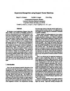
Given a set of independent and identically distributed (iid) training samples, S={(x1, y1), (x2, y2),…..(xn,yn)}, where xi∈ RN and yi∈ {-1, 1} denotes the input and the output of the classification, SVM functions by creating a hyperplane that separates the dataset into two classes. According to the SRM principle, there will just be one optimal hyperplane, which has the maximum distance (called maximum margin) to the closest data points of each class as shown in Fig. 1. These points, closest to the optimal hyperplane, are called Support Vectors (SV). The hyperplane is defined by the equation w.x + b = 0 (1), and therefore the maximal margin can be found by minimizing ½ ||w||2 (2) [5].

yi.(xi.w + b) ≥ 1 , ∀ i (3) The concept of the Optimal Separating Hyperplane can be generalized for the non-separable case by introducing a cost for violating the separation constraints (3). This can be done by introducing positive slack variables ξi in constraints (3), which then becomes, yi.(xi.w + b) ≥ 1 - ξi , ∀ i (4) If an error occurs, the corresponding ξi must exceed unity, so Σi ξi is an upper bound for the number of classification errors. Hence a logical way to assign an extra cost for errors is to change the objective function (2) to be minimized into: min { ½ ||w||² + C. (Σi ξi ) } (5) where C is a chosen parameter. A larger C corresponds to assigning a higher penalty to classification errors. Minimizing (5) under constraint (4) gives the Generalized Optimal Separating Hyperplane. This is a Quadratic Programming (QP) problem which can be solved here using the method of Lagrange multipliers [8]. After performing the required calculations [5, 7], the QP problem can be solved by finding the LaGrange multipliers, αi, that maximizes the objective function in (6), n

W (α ) = ∑αi − i=1

( )

1 n αiα j yi y j xTixj ∑ 2 i, j=1

(6)

subject to the constraints,

0 ≤ αi ≤ C,

i=1,…..,n,

and

∑

n

α i yi = 0.

i =1

(7)

Fig. 1: Optimal Hyperplane and maximum margin for a two class data [6]. The Optimal Separating Hyperplane can thus be found by minimizing (2) under the constraint (3) that the training data is correctly separated [7].

The new objective function is in terms of the Lagrange multipliers, αi only. It is known as the dual problem: if we know w, we know all αi. if we know all αi, we know w. Many of the αi are zero and so w is a linear combination of a small number of data points. xi with non-zero αi are called the support vectors [9]. The decision boundary is determined only by the SV. Let tj (j=1, ..., s) be the indices of the s support vectors. We can write, s

w = ∑ α t j yt j xt j (8) j =1

6th WSEAS International Conference on CIRCUITS, SYSTEMS, ELECTRONICS,CONTROL & SIGNAL PROCESSING, Cairo, Egypt, Dec 29-31, 2007 164

So far we used a linear separating decision surface. In the case where decision function is not a linear function of the data, the data will be mapped from the input space (i.e. space in which the data lives) into a high dimensional space (feature space) through a non-linear transformation function Ф ( ). In this (high dimensional) feature space, the (Generalized) Optimal Separating Hyperplane is constructed. This is illustrated on Fig. 2 [10].

multipliers differ from zero. As such, using the support vector machine we will have good generalization and this will enable an efficient and accurate classification of the sensor signals. It is this excellent generalization that we look for when analyzing sensor signals due to the small samples of actual defect data obtainable from field studies. In this work, we simulate the abnormal condition and therefore introduce an artificial condition not found in real life applications.

2.2 Discrete Wavelet Transform

Fig. 2: Mapping onto higher dimensional feature space By introducing the kernel function, K (xi , x j ) = Φ ( xi ), Φ (x j ) , (9) it is not necessary to explicitly know Ф ( ). So that the optimization problem (6) can be translated directly to the more general kernel version [10], n

W (α ) = ∑ α i − i =1

1 n ∑ α iα j yi y j K (xi , x j ) , 2 i=1, j =1

(10) n

subject to C ≥ α i ≥ 0, ∑ α i yi = 0 . i =1

After the αi variables are calculated, the equation of the hyperplane, d(x) is determined by, l

d ( x ) = ∑ yiα i K( x , x i ) + b i =1

(11)

The equation for the indicator function, used to classify test data (from sensors) is given below where the new data z is classified as class 1 if i>0, and as class 2 if i