Planar configuration for image projection Leon Eisen, Michael Meyklyar, Michael Golub, Asher A. Friesem, Ioseph Gurwich, and Victor Weiss
A flat panel, compact virtual image projection display is presented. It is based on a light-guided optical configuration that includes three linear holographic gratings recorded on one planar transparent substrate so as to obtain a magnified virtual image for a small input display. The principles of the projection display, unique design, and procedures for experimentally recording an actual planar configuration are presented, along with evaluation results. The results reveal that a field of view of ⫾8° can be readily achieved at a distance of 36 cm, making such planar configurations attractive for head-up displays. © 2006 Optical Society of America OCIS codes: 090.2820, 090.2870, 050.1950, 220.4000.
1. Introduction
During the past three decades, there has been significant progress in the areas of holographic imaging and display technology, specifically in holographic head-up display configurations for aircraft and vehicles, where a magnified projected image, viewed through a holographic combiner, overlays the real scene outside.1,2 Current holographic displays are rather bulky because the light from a display source must be reflected from the entire surface of the holographic combiner, requiring a long distance between them, a relatively large lens system, and difficult alignment. Here we present a planar light-guided projection display configuration in which three holographic gratings (HGs) are recorded on a single transparent planar substrate. The input display source can be located close to the substrate, so the overall configuration can be compact. Moreover, the alignment problem is transferred to the recording stage where it is easier to control, and chromatic aberrations can be compensated relatively easily. Similar but simpler planar configurations have already been incorpo-
L. Eisen (
[email protected]), M. Meyklyar, M. Golub, and A. A. Friesem are with the Department of Physics of Complex Systems, Weizmann Institute of Science, P.O. Box 26, Rehovot 76100, Israel. I. Gurwich and V. Weiss are with ELOP ElectroOptics Industries, P.O. Box 1165, Rehovot 76111, Israel. Received 26 July 2005; revised 6 November 2005; accepted 25 November 2005; posted 2 December 2005 (Doc. ID 63534). 0003-6935/06/174005-07$15.00/0 © 2006 Optical Society of America
rated into integrated optical imaging systems3,4 and visor displays.5,6 2. Light-Guiding Configuration and Principle of Operation
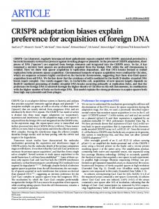
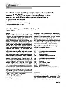
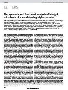
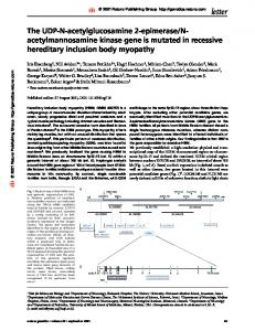
The planar light-guiding configuration is schematically presented in Fig. 1. It comprises three relatively simple linear HGs of different sizes and geometry, all recorded on a single transparent substrate. The first HG H1 couples the light into the substrate, traps it by total internal reflection, and directs it toward the second HG H2, which expands the light along one direction. The second intermediate HG H2 redirects the light distribution toward the much larger third HG H3, which expands light in the other orthogonal direction and decouples it from the substrate outward toward the viewer. To ensure that the output image has a uniform light intensity distribution, the diffraction efficiency at each point of HG H2 and HG H3 must be different. This is achieved with proper design and recording procedures for controlling the diffraction efficiency at each point of HG H2 and HG H3, so as to obtain relatively uniform light distribution at the output over the entire field of view. The dimensions of HGs H2 and H3 depend on the desired lateral pupil magnification in both orthogonal directions at the given distance between the viewer and the output HG H3. An overall result is to allow the viewer (V) to see the virtual image of the input display, with a relatively large field of view, through the large output HG H3. This is illustrated in Fig. 2, where the light from the input display source is collimated so that each point source is converted to an incident plane wave onto the small HG H1 (two such plane waves at extreme points of the source are 10 June 2006 兾 Vol. 45, No. 17 兾 APPLIED OPTICS
4005
Fig. 1. Basic planar light guiding configuration. Light trapping in a virtual display system.
shown). The plane waves propagate by total internal reflection toward HG H3, so the viewer sees the magnified virtual image of the input display at infinity. Essentially, the small input pupil is magnified when viewed through HG H3; the magnification is given by the size of HG H3 over that of HG H1. It should be noted that the plane waves for two angles as indicated in Fig. 2 are discrete and do not overlap in order to simplify the description of the operation principle. However, when the entire range of angles within the field of view and thin light-guiding substrate are exploited, there will be a continuous and relatively uniform image projected into the eye. Now, HG H1 diffracts the normally incident light to an angle diff, so the diffracted light propagates inside the substrate by total internal reflection along the x axis. Accordingly, the grating function of H1 is ⌽1 ⫽ ⫺
2 n sin diff兲x, 共 sub
(1)
where nsub is the refractive index of the substrate and is the wavelength of the incident light. The HG H2 must now redirect the light by 90°, so it will propagate inside the substrate along the orthogonal y axis. Hence the grating function of HG H2 has to have a phase function identical to ⌽1 in the y direction that can be mathematically expressed as 2 ⌽2 ⫽ ⫺⌽1 ⫹ n sin diff兲y 共 sub
冉
冊
冑2 冑2 2 冑2 nsub sin diff x⫹ y 2 2 2 ⫹
冉
冊
冑2 冑2 2 冑2 nsub sin diff x⫹ y . 2 2 2
(2)
Therefore the grating that has the phase function ⌽2 can be achieved by recording the pattern resulting from the interference of two plane waves that are oriented at angles of ⬘ ⫽ ⫾共冑2兾2兲sin共diff兲 with respect to the normal of the recording substrate and, in addition, the grating vector must be normal to the bisector of the angle between the x and y axes. The grating function of HG H3, identical to ⌽1 but along the y axis, is 4006
⌽3 ⫽ ⫺
2 n sin diff兲y. 共 sub
APPLIED OPTICS 兾 Vol. 45, No. 17 兾 10 June 2006
(3)
Combining Eqs. (1)–(3) yields ⌽1 ⫹ ⌽2 ⫹ ⌽3 ⫽ 0.
(4)
Equation (4) indicates that the total configuration does not add phase, other than multiple integers of , to an incoming beam. Furthermore, Eq. (4) is valid for all wavelengths, so the overall optical configuration will have no chromatic dispersion and is therefore appropriate for the polychromatic light. Typically, the output light emerges in a direction either the same as or opposite of that of the incoming light. 3. Design Procedure
To determine the desired grating period of HG H1 and HG H3 for a specific field of view, we start with the basic equation for a diffraction grating in classical mounting, nsub sin diff,j ⫽ ⫺ni sin inc ⫹
2 n sin diff x ⫹ nsub sin diff y兲 ⫽ 共 sub ⫽
Fig. 2. Image output pupil magnification principle. IDS, input display source; CL, collimating lens; H1, input coupling grating; H3, output decoupling grating; GS, glass substrate; V, viewer.
j , ⌳x
(5)
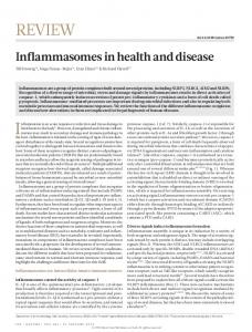
where ⌳x is the grating period, j is the diffraction order number, diff,j are the diffraction angles in the substrate medium with refractive index nsub, and inc is the incidence angle in the upper layer (air) with refractive index ni ⫽ 1. All these parameters are depicted in Fig. 3, which shows the geometry and ray propagation for HG H1 and HG H3. Now, the condition for total internal reflection in the substrate is nsub sin diff,j ⱖ ni.
(6)
Substituting Eq. (5) into Eq. (6) yields sin inc ⱕ
j ⫺ 1. ⌳xni
(7)
Evidently, Eq. (7) defines an available range of inci-
where m ⫽ 1, . . . , M and 1 is the local diffraction efficiency at the first zone. Assuming no losses and taking the local diffraction efficiency at the last zone to be 100%, this yields 1 ⫽
Fig. 3. Geometry and ray propagation of the light-guiding configuration.
dent angles in air. Therefore for a specific field of view the desired grating period can be obtained as ⌳x ⫽
. 1 ⫹ sin共inc兲
Idiff 共m⫹1兲 ⫽ Iinc共m⫹1兲m⫹1 ⫽ Iinc共m兲共1 ⫺ m兲m⫹1 ⫽
Idiff 共m兲 1 ⫺ m兲m⫹1, m 共
(9)
where 共1 ⫺ m兲 is the efficiency of normally reflected light from the mth zone. We then compared intensities of light diffracted at the two consecutive zones, i.e., Idiff 共m⫹1兲 ⫽ Idiff 共m兲, to obtain the following equation for m at the mth zone: m ⫽
1 , 1 ⫺ 共m ⫺ 1兲1
(10)
(11)
As is evident, the local diffraction efficiency behaves as an increasing geometrical function along the lateral coordinate of HG H2 and the initial local diffraction efficiency is determined by Eq. (11). Now, for the case of a relatively large field of view, the number of zones M will vary with incident angles so the local diffraction efficiency at the last zone cannot be 100% for the entire field of view. Hence normally reflected light from the last zone associated with the specific incident angle leads to reduction of the total output power as
(8)
To ensure that the light emerging from the output HG H3 is uniformly distributed, the localized diffraction efficiencies along HG H1 and HG H3 must vary. Accordingly, we developed an algorithm to calculate required diffraction efficiencies at each output point on both the intermediate HG H2 and the output HG H3. We start with the HG H2 case, which could be treated analytically for the infinitely narrow field of view owing to an existence of only two diffraction orders, zero and first. Zero order is associated with the normally reflected light continuously propagating along HG H2, whereas the first order corresponds to the light propagating toward HG H3. For the analysis, HG H2 is divided into M discrete zones, where each zone corresponds to a bounce number m and is assigned the local diffraction efficiency m. Each zone could be considered as a separate grating and the number of such gratings depends on the lateral size of HG H2, substrate thickness, and internal light propagation angle. We denote the intensity of light impinging upon the mth zone as Iinc共m兲 and the intensity of the light diffracted on the mth zone as Idiff共m兲. Then the power balance at the (m ⫹ 1)th zone can be mathematically expressed as
1 . M
冋
册
M 1 Iloss , ⫽ 兿 1⫺ Iinc m⫽1 m ⫺ 1兲1 共
(12)
where Iloss is the intensity of the reflected light from the last zone and Iinc is the total input light. Also, for HG H3, redundant reflected and transmitted diffraction orders exist that can be considered in our configurations as additional losses. Consequently, Eqs. (10) and (11) cannot be satisfied for the entire field of view, and we must resort to a numerical optimization procedure. In this procedure we use the local groove depth in discrete zones 兵hm其m⫽1 M as optimization variables, and Eqs. (10)–(12) for the evaluation of starting points. As a criterion for the optimization, we minimize the integral deviation of local light intensities for different inner propagation angles inside HG H2 and HG H3 from its mean values. For N different N propagation angles, denoted as 兵n其n⫽1 , we chose the criterion as Err ⫽
N
Jn
兺 兺 关Idiff 共i,  兲 ⫺ Idiff共 兲兴 n⫽1 j⫽1 n
n
2
→ min,
(13)
where Idiff 共n兲 denotes the mean value of the local intensity of the diffracted light along the whole grating evaluated for the specific propagation angles and j is the diffraction order number. We illustrate our design procedure for a lightguiding configuration that is illuminated with TE polarized light of wavelength ⫽ 525 nm and has a field of view of ⫾8°. In accordance with Eq. (8), the grating period ⌳x for HG H1 must be less than 460 nm, so for convenience we chose ⌳x ⫽ 450 nm. We also assume that the groove slant angle of HG H1 is 17° in order to obtain reasonable diffraction efficiency. The analysis of the recording of slanted surface relief gratings in photoresist has been described elsewhere.7 We then calculated the diffraction efficiency as a function of groove depth for several incidence angles on HG H1 using rigorous coupled wave 10 June 2006 兾 Vol. 45, No. 17 兾 APPLIED OPTICS
4007
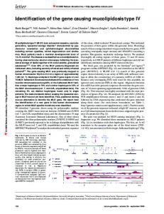
Fig. 4. Calculated diffraction efficiency as a function of groove depth for different incidence angles on HG H1 with sinusoidal surface relief grating profile and grooves slanted at 17°. The incident light is TE polarized.
analysis (RCWA).8 The results of these calculations are presented in Fig. 4. As shown, the highest diffraction efficiency of approximately 20%–25%, and still with good uniformity within the field of view, may be achieved for a groove depth of approximately 0.17–0.20 m. Now, HG H2 receives the light from HG H1 and redirects the beams toward HG H3. For a 90° redirection of light inside the substrate, the period of HG H2 must be 冑2兾2 that of HG H1.9 Specifically, when the grating period of HG H1 is 450 nm, then that of HG H2 is 318 nm, leaving only the zero and first diffraction orders as nonevanescent. For such HG H2, in a conical mounting configuration, the calculated maximum local diffraction efficiency is less than 12%, even with an idealized situation of optimized groove depth, no scattering, and no absorption. Assuming a more practical maximum local diffraction efficiency of approximately 2,M ⫽ 6.0% and M ⫽ 11 bounces, we obtain a total diffracted light efficiency of HG H2 from all bounces of tot ⫽ 40.7%. HG H3 consists of M local gratings of the same
Fig. 5. Geometry, showing the various local reflections and diffractions in HG H3. 4008
APPLIED OPTICS 兾 Vol. 45, No. 17 兾 10 June 2006
Fig. 6. Calculated local groove depth, local diffraction efficiency, and local light power as a function of the number of bounces for HG H3 with sinusoidal surface relief grating and grooves slanted at 17°. The calculations are optimized for reflection mode and TE polarization. (a) Local depth of groove; (b) local diffraction efficiency; (c) local light power distribution.
period as that of HG H1, each with a different diffraction efficiency, so the overall output light is uniform. The task of designing HG H3 with differing local diffraction efficiencies is much more complicated than designing HG H2 because several reflection order diffractions are present in the diffraction process, as depicted in Fig. 5. As shown, reflection order 0R describes the continuation of trapped light propagation in the substrate; reflected diffraction order 1R corresponds to the output light decoupled from the opposite (no grating), smooth side of the substrate (reflection mode of HG H3); transmitted diffraction order 1T corresponds to the output light decoupled from the substrate side covered with the grating (transmission mode of HG H3); and the reflected diffraction order 2R corresponds to a diffraction order. The balance of light powers for HG H3 is therefore more complicated than for HG H2. The power that continues to propagate is not just what is left after decoupling outward from the grating. There are also additional losses due to back-diffracted light, and the fact that decoupling occurs to both sides of the substrate must also be taken into account. We calculated the optimized local groove depth for HG H3 with the same period and the same groove slant angle as HG H1 and then used these depths to calculate the local diffraction efficiency and local output light power. The results are presented in Fig. 6. Figure 6(a) shows the optimized local groove depth as a function of the bounce number, Fig. 6(b) shows the optimized local diffraction efficiency, and Fig. 6(c) shows the local output light power. Summing all the local output light powers, we found that the throughput efficiency could potentially reach 36%–40% for this HG H3. 4. Experimental Procedure and Results
To verify our design procedures and calculations, we experimentally recorded a light-guiding configuration with three surface relief gratings.7 The gratings were recorded in an Ultra-I 123 photoresist layer on a glass substrate of 3 mm thickness. The size of the
Fig. 7. Calculated and experimental diffraction efficiency as function of input incident angle for HG H1.
Fig. 8. Calculated and experimental local diffraction efficiency (DE) for HG H2.
input HG H1 was 7.5 mm ⫻ 7.5 mm and the size of the output HG H3 was 75 mm ⫻ 75 mm. HGs H1 and H3 were recorded with asymmetric offset angles so as to obtain grooves with a 17° slant and a grating period of about 450 nm. HG H2 was recorded with symmetrical grooves and a grating period of about 318 nm. To obtain the needed variable local diffraction efficiency for HG H2 and HG H3, we varied the local exposure by means of a slowly moving opaque mask, so that each location on the photoresist layer had a different exposure energy. The specific local exposure energy depended on the velocity of the movable mask as a function of lateral dimensions of HG H2 and HG H3. We measured the diffraction efficiency, i.e., the power in the first diffraction order over that of the incident light, as a function of incident angle for HG H1, both for TE and TM polarization. The readout wavelength was 514.5 nm. The experimental results along with calculated results are presented in Fig. 7. As is evident, the diffraction efficiency is higher for TE polarization than for TM polarization, and there
Fig. 9. Calculated and experimental local diffraction efficiency (DE) for HG H3 at the center of the field of view. 10 June 2006 兾 Vol. 45, No. 17 兾 APPLIED OPTICS
4009
Fig. 11. Experimental output imagery as viewed through HG H3. The thickness of the light-guiding substrate was 3 mm.
Fig. 10. Experimentally measured relative output light power distribution as a function of location on HG H3 for three different incident angles at HG H1. (a) inc ⫽ 0°; (b) inc ⫽ ⫺8°; (c) inc ⫽ 8°.
4010
APPLIED OPTICS 兾 Vol. 45, No. 17 兾 10 June 2006
is good agreement between the experimental and calculated results. We then measured the localized diffraction efficiency of HG H2. This was done by measuring the power of the diffracted light at sequential internal bounces and dividing it by the power of the incident light that arrives at an oblique angle from HG H1. First, we measured the light diffracted at the first bounce toward HG H3, as well as the power of the normally reflected light that continues to propagate in the substrate along HG H2. Then we repeated such measurements at all subsequent bounces along HG H2 and used the measured values of diffracted and reflected light to determine the localized diffraction efficiencies along HG H2. The results are presented in Fig. 8, along with the designed local diffraction efficiencies. As can be seen, there are discrepancies between the designed and measured local diffraction efficiencies. We attribute these mainly to undesired absorption and light scattering in the photoresist layer. Finally, we measured the local diffraction efficiency of HG H3 at the center of the field of view. The results are presented in Fig. 9, along with the designed local diffraction efficiency. Here again it is evident that the experimental results are uniformly lower than the calculated designed ones. We believe that this reduction of local diffraction efficiency is mainly due to undesired absorption and scattering, which were not accounted for in the theoretical calculations. We also measured the output light intensity distribution, emerging from HG H3, for three different input incident angles of 0°, ⫹8°, and ⫺8°. The results are presented in Fig. 10. Figure 10(a) shows the measured relative output light power as a function of location along HG H3 for the normally incident readout light, Fig. 10(b) for readout light incident at ⫺8°,
and Fig. 10(c) for readout light incident at ⫹8°. The data in each graph is normalized with respect to the maximum value obtained for the normally incident light. These results indicate that it is indeed possible to obtain relatively uniform light distributions from the output grating for the required field of view. The overall throughput light efficiency and uniformity was measured for several samples. The efficiencies ranged from 1.0% to 2%, with light uniformity best at the lower efficiencies. The representative magnified imagery, viewed through HG H3, is depicted in Fig. 11. This imagery was obtained for a light-guiding configuration, where the dimensions of HG H1 were 1 cm ⫻ 1 cm, HG H3 10 cm ⫻ 10 cm, and the thickness of the substrate was 3 mm. 5. Concluding Remarks
We presented the design, recording procedures, and results of a new light-guiding planar configuration for obtaining a large virtual image. In the configuration three simple linear holographic diffraction gratings are recorded on a single planar substrate, so as to form a compact and robust optical projection system. Our results reveal that with an output grating of 10 cm ⫻ 10 cm, a field of view of ⫾8° at a distance of 36 cm can be readily achieved. We expect that such a planar configuration could operate well with both monochromatic and polychromatic display illuminations and could be exploited for a variety of head-up display applications. The authors thank Piermario Repetto of the Centro Ricerche Fiat for a constructive collaboration within
the Optoelectronic Eye-up Floating Display Bus (OEDIBUS) project and acknowledge the financial support by the European Commission for the same project under contract IST-1999-20394. References 1. R. Wood and M. Hayford, “Holographic and classical head-up display technology for commercial and fighter aircraft,” in Holographic Optics: Design and Applications, I. Cindrich, ed., Proc. SPIE 0883, 36 –52 (1988). 2. R. L. Fisher, “Design methods for a holographic head-up display curved combiner,” Opt. Eng. 28, 616 – 621 (1989). 3. S. Sinzinger and J. Jahns, “Integrated micro-optical imaging system with a high interconnection capacity fabricated in planar optics,” Appl. Opt. 36, 4729 – 4735 (1997). 4. A. Friesem and Y. Amitai, “Planar diffractive elements for compact optics,” in Trends in Optics, A. Consortini, ed. (Academic, 1997), pp. 125–144. 5. W. Jiang, D. L. Shealy, and K. M. Baker, “Physical optics analysis of the performance of a holographic projection system,” in Diffractive and Holographic Optics Technology, Proc. SPIE 2404, 1236 –1240 (1995). 6. Y. Amitai, S. Reinhorn, and A. A. Friesem, “Visor display design based on planar holographic optics,” Appl. Opt. 34, 1352–1356 (1995). 7. I. Gurwich, V. Weiss, L. Eisen, M. Meyklyar, and A. A. Friesem, “Design and experiments of planar optical light guides for virtual image displays,” Proc. SPIE 5182, 212–221 (2003). 8. G. Moharam and T. K. Gaylord, “Diffraction analysis of dielectric surface-relief grating,” J. Opt. Soc. Am. 72, 1385–1392 (1982). 9. R. Shechter, Y. Amitai, and A. A. Friesem, “Compact beam expander with linear gratings,” Appl. Opt. 41, 1236 –1240 (2002).
10 June 2006 兾 Vol. 45, No. 17 兾 APPLIED OPTICS
4011