Abstract: A new method for plane hypothesis generation based on a sweeping process is presented. The method is feature based in contradiction to earlier ...
Plane parameter estimation by edge set matching Joachim Bauer∗ , Konrad Karner∗ and Konrad Schindler† ∗
†
VRVis Research Center for Virtual Reality and Visualization email: {bauer,karner}@vrvis.at Institute for Computer Graphics and Vision, Graz University of Technology email: {schindl}@icg.tu-graz.ac.at
Abstract: A new method for plane hypothesis generation based on a sweeping process is presented. The method is feature based in contradiction to earlier methods which rely on image correlation. The features used are edgel elements (’edgels’) which are extracted in a preprocessing step. The experiments show an improvement in speed as well as in accuracy.
1
Introduction
The automatic generation of 3D models from digital images is a popular topic. Especially in the field of city modeling, where huge amounts of data have to be processed, a high degree of automation is desirable. The work-flow of our system is shown in Figure 1. In this paper we discuss the gray shaded parts, which describe a feature based algorithm for 3D plane hypothesis generation based on a sweeping process. A set of images with known exterior orientation together with extracted 2D lines are the input data. A line matching method is applied to generate 3D line hypothesis and subsequent plane based homographies for image pairs. Using the homographies the edgel sets in the vicinity of the projected 3D lines are swept in order to detect the optimal orientation of the half planes. The sweeping process is also used to validate the 3D line hypothesis. Our approach is based on image features, namely edgels, instead of using plain image information as in earlier approaches by Zissermann et al. [6] and Baillard et al. [1]. The method is also comparable to the technique described by Coorg and Teller in [2]. The advantage is a significant speedup and better geometrical accuracy. Results using our algorithm on a set of synthetic images and a sequence of real images are presented.
2
Line matching
Our approach for the computation of a 3D line set, using oriented images and extracted 2D lines, closely follows the one described by Schmid and Zisserman [5]. Multiple images of a scene together with extracted 2D line segments are used to compute and verify 3D line hypotheses. The algorithm uses both, the geometrical information of the 2D line segments
Figure 1: Sketch of the work flow: On the left side the feature extraction work flow is visualized, on the right side the 3D modeling pipeline is depicted. The grey shaded areas are discussed in this paper.
and the photometric information of the corresponding images. The result of the line matching process is a set of 3D line segments in object space.
3
Plane sweeping
The process of plane sweeping is discussed in [6] and [1] and will only be briefly sketched here. The main difference is the use of a similarity function based on edgel point sets instead of computing the similarity via image correlation for interest points. The 3D lines are used to generate planes hypothesis from which the plane homographies between image pairs are computed. The homographies induced by the sweeping plane are represented as a 3 × 3 homography matrix H and allow direct point transform between images of a planar region. This means that the edgel point sets A of the planar region captured by the first cameras image can now be directly transformed to its corresponding view A˜ for the second cameras image. This is done by multiplication with the given homography matrix: A˜ = HA. The mathematical framework is presented in the following subsection. 3.1
Homographies from planes
The computation of the homographies for a planar region captured from two different views is described in this section. The plane is defined by its normal vector n and distance to origin d. T is the transformation matrix from world coordinates to a coordinate system in the 3Dplane (x, y, 0), where the plane defines the x, y-plane and the x-axis is horizontal in the world coordinate system.
T =
cos α − sin α 0 0 sin α cos κ cos α cos κ − sin κ 0 sin α sin κ cos α sin κ cos κ −d 0 0 0 1
with α = − π2 − λ, λ = arctan nnxy and κ = ϕ − π2 , ϕ = arctan √ n2z
nx +n2y
.
Given T , the homography from plane to second retina is x2 = P 2 ∗ (T −1 )red ∗ xplane where
(T −1 )red = T −1 ∗
1 0 0 0
0 1 0 0
0 0 0 1
h i −1 −1 −1 T(2) T(4) = T(1)
The homography from the first retina to the plane is given by T ∗C ∗ (T ∗ P 1+ )(3) ) ∗ x1 (T ∗ C)(3)
xplane = (T ∗ P 1+ −
where the camera matrix C is C = −M −1 ∗ p4with P 1 =
h
i M |p4 .
and P 1+ is the pseudoinverse of P 1. (T ∗ C)(3) =
h
0 0 1 0
i
∗T ∗C
and +
(T ∗ P 1 )(3) =
h
0 0 1 0
i
∗ (T ∗ P 1+ )
denotes the third row of the respective matrices. The total homography therefore is defined as x2 = P 2 ∗ (T −1 )red ∗ (T ∗ P 1+ −
T ∗C ∗ (T ∗ P 1+ )(3) ) (T ∗ C)(3)
3.2
Similarity measure for point sets
With the homographies given, we are able to transfer edgel sets in the vicinity of the projected 3D lines and measure the degree of similarity. The similarity between two point sets A˜ and B, where A˜ is the transformed edgel point set of the first image, is measured by summing up the squared distances of every edgel point a ∈ A to its closest neighbor b ∈ B. Using a squared distance measure discriminates points that are far from each other automatically. For fast location of the nearest neighbor the 2D edgel sets are stored in a KD-tree. 3.3
Sweeping modes
In this section the different sweeping modes are explained. There are two possible sweeping modes: a rotational sweep mode and a translational sweep mode. Figure 2 shows an illustration of the two modes. The rotational sweep in this example is performed for the eave line of the captured facade (the camera is symbolized as a pyramid) and the translational sweep is performed for the whole facade.
(a)
(b)
Figure 2: Illustration of the two sweeping modes (the camera is symbolized as a pyramid). (a) rotational sweep planes for the eave line of the facade (b) translational sweep planes
3.3.1 Rotational sweep In case of the rotational sweep a 3D line serves as rotational axis for a set of plane hypothesis. The 2D edgels which are transformed during the sweeping process are taken from the neighborhood of the projected 3D line from the first image and actually split into two edgel sets on both sides of this 2D line are extracted. Assuming a planar patch on at least one side of the line, one of the two edgel sets will be aligned. In the next step an initial hypothetical sweeping plane using the 3D line and the origin of the camera is instantiated. In the following sweeping step the plane is rotated around the axis formed by the two points of the 3D line. In order to avoid extreme conditions at the start of
the sweeping process, when viewing the plane nearly edge on, it is first rotated to a reasonable start position by a fixed angle ϕmin . This condition is also met at the end, so the sweep angle range for the plane is ϕmin ≤ ϕ ≤ 180o − ϕmin degrees. The plane hypothesis at the start position, two of the subsequent planes and the end position are shown in Figure 2(a). 3.3.2 Translational sweep For the translational sweep the plane hypothesis is not induced by a 3D line but by the normal vector and a 3D point, this point however can be an endpoint of a 3D line. The normal vectors are computed from the 3D lines by clustering, but can also be determined from at least two known vanishing points [4]. The input for the clustering are crossproduct vectors from 3D line pairs, where only line pairs with a reasonable large inner product are considered. In contradiction to the rotational sweep, where the sweep range is bounded, the translational sweep is only bounded at one side, the camera origin. The second bound must be determined from the scale of the modeled scene e.g. from the extend of the 3D lines. This initial plane is then swept along the direction of the normal vector. Figure 2(b) shows three plane hypothesis for the dominant facade. 3.4
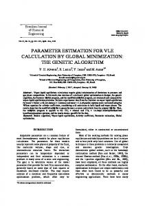
Sources of error
The orientation of the detected planes in sweeping mode is sometimes slightly inaccurate, caused by the fact that detected 3D lines do not lie exactly on the plane. In case of architectural models 2D lines often are detected on topological features that stand out of the facade plane such as window sills and friezes or lie behind the facade plane e.g. window frames. In this case the final orientation of the plane does not match the normal vector of the facade. Figure 3 shows the scenario: A 3D line is detected on a protruding window sill; The best alignment found for the plane is intersecting the facade. Another problem are 3D lines with an inaccurate orientation, for those lines the planes are also slightly inaccurate. With the translative sweeping approach it is possible to overcome the problems described above, since the normal vector for a translative sweep is computed by clustering.
4
Experiments
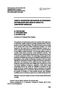
We conducted several experiments with synthetic as well as real image data. In Figure 4 the sweeping process for synthetic data is shown. Figure 5 shows the detected plane for the synthetic data. The next experiment compares the image based methods versus the feature based approach. Figure 6 shows the score values plotted against the sweep angle. The score for the feature based method is plotted solid, the score for the image based method is dotted. Multiple maxima,
plane
facade
3D line
Figure 3: The new edgel based approach vs. the image based approach. Note the significant sharper peak for the feature based method.
1
0.9
0.8
0.7
(a)
(b)
sweep score
0.6
0.5
0.4
0.3
0.2
0.1
0
(c)
(d)
0
20
40
60
80 sweep angle
100
120
140
160
(e)
Figure 4: Alignment of edgel sets for a 3D line. (a) template edgel sets left (light crosses) and right (dark crosses)from a projected 3D line. (b) transformed left edgel set at 40o and (c) 60o (d) final alignment of the left edgel point set (d) sweep scores for both edgel point sets (dashed and solid) over the sweep range (20o − 160o ).
caused by repeating patterns on the facade, make it difficult to detect the best maximum for the image based approach. The score function for the image based approach gets smoother if a larger correlation window is used, in our experiments the size of the correlation window was 19.
(a)
(b)
(c)
1
1
0.9
0.9
0.8
0.8
0.8
0.7
0.7
0.7
0.6
0.6
0.6
0.5
score
1
0.9
score
score
Figure 5: Synthetic input data and resulting plane hypotheses, note the accurate alignment of the planes. (a) synthetic input image; (b) view from the left side; (c) view from the right side;
0.5
0.5
0.4
0.4
0.4
0.3
0.3
0.3
0.2
0.2
0.2
0.1
0.1
0
0
10
20
30
40 50 sweep angle
60
70
80
90
0
0.1
0
10
20
30
40
50 sweep angle
60
70
80
90
100
0
0
20
40
60 80 sweep angle
100
120
140
Figure 6: The new edgel based approach vs. the image based approach. Note the significant sharper peak for the feature based method.
Accuracy investigations complete the series of experiments. These experiment was carried out using synthetic data which known ground truth. Table 4 shows a comparison of the image based method versus the feature based approach. The error between the normal vector of the detected plane and the correct normal vector is used to compare the accuracy of the two methods. The experiments were carried out on images corrupted with different levels of gaussian noise using 23 planes. The feature based method performs better than the image based algorithm especially if the images are corrupted with noise. Our method is about twelve times faster than the image based approach, though there was no effort made to optimize the image based method for speed.
5
Summary and Future Work
We presented an improved method for plane hypothesis generation using a feature based plane sweeping approach. The experiments showed that the feature based approach is faster than the image based method and yields also more accurate results. As mentioned in section 3.4 errors are mainly caused by 3D lines that are not lying on the plane. A solution for this
% noise Feature based Image based Feature based Image based Feature based Image based
0 0 2 2 5 5
mean error std. deviation 0.8736 2.0568 0.9216 2.0378 1.4808 3.2758
1.1087 7.52 0.9873 8.1545 5.4877 11.4760
Table 1: Feature based method vs. Image based method. The error is the difference between correct normal vector and the normal vector of the detected plane. (23 planes were used in this experiment)
problem could be a final alignment of the point set with an optimization method proposed by Fitzgibbon [3].
Acknowledgments This work has been done in the VRVis research center, Graz and Vienna/Austria (http://www.vrvis.at), which is partly funded by the Austrian government research program Kplus.
References [1] Caroline Baillard, Cordelia Schmid, Andrew Zisserman, and Andrew Fitzgibbon. Automatic line matching and 3d reconstruction of buildings from multiple views. In ISPRS Conference on Automatic Extraction of GIS Objects from Digital Imagery, IAPRS Vol.32, Part 3-2W5, pages 69–80, September 1999. [2] S. Coorg and S. Teller. Extracting textured vertical facades from controlled close-range imagery. In CVPR, pages 625–632, 1999. [3] Andrew W Fitzgibbon. Robust registration of 2d and 3d point sets. In Proceedings, British Machine Vision Conference, 2001. [4] F. Schaffalitzky and A. Zisserman. Planar grouping for automatic detection of vanishing lines and points. Image and Vision Computing, 18(9):647–658, June 2000. [5] C. Schmid and A. Zisserman. The geometry and matching of lines and curves over multiple views. IJCV, 40(3):199–233, December 2000. [6] A. Zisserman, T. Werner, and F. Schaffalitzky. Towards automated reconstruction of architectural scenes from multiple images. In Proc. 25th workshop of the Austrian Association for Pattern Recognition, pages 9–23, 2001.