European Association for the Development of Renewable Energies, Environment and Power Quality (EA4EPQ)
International Conference on Renewable Energies and Power Quality (ICREPQ’11) Las Palmas de Gran Canaria (Spain), 13th to 15th April, 2011
Planning of power systems with distributed generation and storage C. Ponce-Corral1, H. Bludszuweit2, and J.A. Domínguez-Navarro3 1
Institute of Engineering and Technology, UACJ (Universidad Autónoma de Ciudad Juárez) Henri Dunant #4016, Zona Pronaf, Ciudad Juárez, México, C.P. 32310 Phone number:+0052 656 6882100, e-mail:
[email protected] 2
CIRCE Research Institute, University of Zaragoza Campus Río Ebro – C/Mariano Esquilor Gómez, 15, 50018 Zaragoza (Spain) Phone number:+0034 976 765184, e-mail:
[email protected] 3
Department of Electrical Engineering, C.P.S., University of Zaragoza Campus Río Ebro – C/ María de Luna, 3, 50018 Zaragoza (Spain) Phone number:+0034 976 762401, e-mail:
[email protected]
It may be that small generators scattered across the distribution networks would cause alterations in these networks or conversely have a beneficial effect. Therefore, the location of distributed generation is an important aspect of network planning. As stated in [3] a distributed generator is connected to a distribution system, and it will produce energy right there, which changes the traditional power distribution system radically. In this sense it is important to verify that the quality of service is not affected. Poor or no planning can result in obtaining a massive loss of power [4], or serious disturbances in the network, which would adversely affect the quality of supply. In [5] and [6] the importance of good planning is emphasized and the need to develop efficient algorithms that simplify that task is pointed out.. The influence of storage units in electricity networks is addressed by some authors. Researches in [7] carried out the optimization of a distribution system where conventional generators and non-conventional generators with random characteristics are considered. Storage units are included to withstand periods where nonconventional generators are not present. Others authors [8] describe a model to solve the optimal power flow in a power system, which includes wind farms and hydro storage units owned by independent power producers. Paragraph 2 describes the mathematical model used here for distributed generation and storage in electricity networks. In paragraph 3, results are presented which were obtained during the planning horizon. It is confirmed a progressive increase in the penetration of distributed generation and storage units.
Abstract.
A high penetration of distributed generation in electricity networks makes it necessary to adapt the network to the new conditions of generation and consumption. Storage units can be converted within a few years in another element of power grids. Therefore, it is necessary to analyze the network to determine the optimal location of distributed generation, which lines need to be built or where to install the storage units. This paper presents a model of power network planning which takes into account the effect of the expansion of distributed generation. The results obtained show the continuing replacement of conventional generation by distributed generation and the importance of storage units in this process of replacement.
Key words Electric network planning, optimization, storage
distributed
generation,
1. Introduction In recent years, the way of generating electricity has been changing. In the past, all energy was generated in large power plants (hydro, fossil fuel and nuclear). This energy needs to be transported over long distances to consumption centers. The emergence of new technologies that make efficient and cost effective electricity production on a smaller scale, allows the placement of this distributed generation of throughout the entire network, which is a fundamental difference, compared to the traditional approach. The introduction of any generation in these networks has changed some well established concepts . As mentioned in [1] and [2] the inclusion of renewable energy in today's society has caused the change in the way of making Electric Power Systems.
https://doi.org/10.24084/repqj09.452
2.
Mathematical model
The planning model is based on minimizing the cost function, subject to several technical constraints such as balance of power flows in nodes, energy balance in 784
RE&PQJ, Vol.1, No.9, May 2011
storage devices, operation limits of generators, capacity limits of power lines and substations, and maximum voltage drop at nodes. Further details about the model can be found in [9].
1
perf_w perf_pv perf_mgh
0.8 0.6
A. Demand, generation and storage models
0.4
The introduction of storage devices makes it necessary to consider models for demand, generation and storage based on stages. Among these stages an exchange of energy flow is established that charges and discharges these storage devices. In this work, it had been chosen a model of “worse day” with several periods for demand, generation and storage. The demand model can be represented by an annual average profile. In the presented study a standard profile has been considered as the basis of demand behavior. To apply it to different nodes, the standard profile is multiplied by the average demand for each node and a normally distributed noise is added.
0.2 0 0
Optimal planning of distributed generation in distribution networks is formulated here as an optimal monoobjective model, which minimizes the cost and is subject to a set of constraints. The planning process should ensure that distributed generation is sized optimally for the proposed planning horizon, considering that at any stage of its planning horizon the system operation is optimal. The objective function to be minimized is the total cost along the planning horizon in this case 20 years. Constraints depend on the system operation in each period. Distribution substations and renewable distributed generators are responsible for providing the power required by the consumer centers. The substations can supply a maximum power limited by the capacity of distribution transformers. Renewable generators have also associated a maximum power that depends on their technical characteristics, a fixed cost that depends on its nominal power and a variable cost that depends on its maintenance. The lines have associated fixed costs and variable costs. The fixed costs depend on their length and variable costs depend on their transmission losses. In the first year, the whole distribution system is set up, under the condition that no distributed generation and no storage are present. As a result, lines are sized according to the load flows and the associated annualized costs are calculated. From the second year onwards, the installation of distributed generation and storage is allowed, but no additional lines can be added. The installation cost of the new capacity is annualized and added to the costs originated from the first year, and so on. For every year, the sum of these annualized costs is is divided by the annual minimized. If this annual cost can be demand of energy , the cost of energy calculated for every year of the planning horizon as shown in (6). This way, the evolution of the minimized is obtained in €/kWh.
Noise 30% 0.0
‐0.5 12
18
24
Hour of day
Fig. 1. Normalized standard profile to demand model.
The renewable generation profiles shown in Fig. 2 were obtained from historical data. The average of the data is kept in the models, but adverse situations that may be compensated by the storage units are introduced. In the case of wind resource an annual average of 25% of installed capacity is assumed. In addition, a peak that reaches 100% of nominal power at night and a minimum of 0% in the afternoon are assumed, thus simulating the worst scenario when there is always a maximum generation when demand is lowest and vice-versa. In the case of solar resource, the base profile was taken from the annual mean day of radiation. To simulate here the worst case, it is introduced a peak of 100% followed by a minimum of 0% during midday. In another period, power is adjusted to comply with the annual average of about 19% of the peak power, which corresponds to a resource of about 1660 kWh / kWp installed power. Finally, the profile for hydropower resource is similar to the wind profile. Here the annual mean is 30% of installed capacity and the assumed minimum at night is 10% of generation, insead of zero.
https://doi.org/10.24084/repqj09.452
24
B. Optimization problem
Base Profile
6
18
Fig. 2. Normalized renewal generation profiles.
Profile
0
12 Hour of day
1.0
0.5
6
(1) is the cumulated annualized cost after years, Where is the energy demand in year . The cost of each element in period t is derived by adding the fixed costs CF and variable costs CV per period t and annualized to present with the coefficient van.
785
RE&PQJ, Vol.1, No.9, May 2011
,
,
,
, ,
set of all generators in the network ( G(n) is the generator set in node n ), L set of all lines in the network ( L(n) is the lines set to start or end at node n ), S set of all storage devices in the network ( S(n) is the storage devices in node n ), T set of time periods, N set of network nodes, fgeni,t total cost of generator i in period t, flinj,t total cost of line j in period t, fstok,t total cost of storage device k in period t, complex demand at node n in period t, , complex power flow at line j in period t, , power loss at line j in period t, , complex power at generator i in period t, , , , , charge and discharge power of storage device k in period t, power loss at storage device k in period t, , , , , , charge state of storage device k in period (t-1) and period t, , , , charge and discharge energy of storage device k in period t, , operation limits of generator i, , operation limits of line j, , operation limits of storage device k, , , voltage limits at nodes.
(3)
, ,
G
(2)
,
(4)
,
Where: fgeni,t , total cost of generator i in period t, flinj,t , total cost of line j in period t, fstok,t , total cost of storage device k in period t, Energy supplied by the network substation Eq,i,t in kWh comes from different sources, whether conventional or renewable. If the energy price is PE in € / kWh, then the cost of this energy in each time period t is: ·
,
(5)
,,
Where: escalation factor of the energy price. energy price in € / kWh imported from the network in period . set of nodes . set of substations . imported energy from network in kWh from ,, substation at node at period . The mathematical formulation of the problem is: min
,
,
3. Results
,
(6)
The study case is a distribution network of 15 nodes and 14 lines. The distribution substation is located at node 1 and has a capacity of 30 MVA, 115/10 kV. The main line is a double-circuit of 3X1X400Al and branch lines are single circuit of 3X1X400Al. The network topology is shown in Figure 3, network data are in Table I, demand data in Table II.
,
Suject to: - power balance in each node n, ,
,
,
,
(7) ,
,
,
8 kW
- charge state of storage device ,
,
,
10
,
- operation limits of each generator i
26 kW
(8)
,
9
G,
1
14
102 kW
2
3
5
4
242 kW
(9) - operation limits of each line j
L,
108 kW 7 148 kW
(10) - operation limits of each storage device k
62 kW 11 132 kW
41 kW 8
S,
15 135 kW
12 76 kW
57 kW
(11)
13
(12) - voltage limits of each node n
96 kW 6
16 kW
N,
Fig. 3.
Topology of distribution network.
(13) where:
https://doi.org/10.24084/repqj09.452
786
RE&PQJ, Vol.1, No.9, May 2011
Table I. - Network data of 14 lines. Line (ni-nj) 1-2 2-3 3-4 4-5 2-9 9-10 2-6 6-7 6-8 3-11 11-12 12-13 4-14 4-15
R(ohm) 0.0000176 0.0000309 0.0006170 0.0001235 0.0006170 0.0001235 0.0006170 0.0001235 0.0001235 0.0006170 0.0001235 0.0001235 0.0001235 0.0001235
PC(kW) Length(m) 350 265 200 229 100 165 50 206 100 272 50 228 100 345 50 147 50 169 100 242 50 330 50 272 50 301 50 161
The model resolution is carried out using the GAMS programming software and the solver XPRESS. Figure 4 shows the evolution of costs of energy (COE) over the planning horizon in the three scenarios. In the first scenario, when the demand requirements are supplied solely by the distribution network (“Conventional”), the energy cost is increasing from 0.13 to 0.30 € / kWh in 20 years. With the introduction of distributed generation in the network COE rises more slowly up to 0.15 € / kWh in year 20. In the third scenario, when storage is considered, from year 7 onwards COE decreases down to a value of 0.095 € / kWh. The sudden decrease is due to the fact that storage starts to be implemented at that moment, because it has become profitable to install it. It shall be mentioned, that a 20% annual decrease of installation costs has been considered here, and after 7 years costs have fallen enough to make storage profitable.
Z(ohm) 1.3235 1.1446 0.8227 1.0276 1.3579 1.1377 1.7249 0.7340 0.8441 1.2111 1.6515 1.3579 1.5047 0.8074
Table II. – Demand data (kW) in the network of 15 nodes.
1 2 3 4 5 6 7 8 9 10 11 12 13 14 15
t0 0 0 0 0 0 0 0 0 0 0 0 0 0 0 0 t12 0.0 134.3 120.6 68.1 289.9 45.2 182.2 77.3 114.4 8.6 116.2 129.1 17.8 123.4 24.8
t1 0.0 122.9 161.9 93.6 194.4 22.7 111.5 76.7 96.8 8.0 173.9 39.6 15.2 83.9 37.8 t13 0.0 117.3 135.1 98.0 255.8 38.9 206.8 72.2 110.0 9.5 207.4 89.5 18.4 149.2 31.0
t2 0.0 52.0 79.0 30.6 276.7 57.8 112.0 40.2 101.2 8.0 105.5 83.3 13.9 186.0 7.7 t14 0.0 106.1 78.2 77.3 379.8 41.6 115.6 59.0 135.1 9.3 176.6 90.5 15.9 192.6 42.0
t3 0.0 98.8 2.1 68.3 149.1 56.8 143.1 82.1 89.5 7.9 87.1 51.4 6.6 134.3 24.6 t15 0.0 160.7 129.6 74.2 399.3 69.4 122.9 66.8 111.8 15.0 115.5 73.8 7.3 128.0 10.7
t4 t5 0.0 0.0 115.2 100.8 64.4 80.6 29.6 40.8 221.7 317.1 34.5 35.8 135.9 106.4 62.4 20.4 80.3 156.3 8.6 4.5 82.7 145.3 50.3 48.7 22.1 7.1 136.6 43.4 22.7 14.2 t16 t17 0.0 0.0 131.6 78.3 91.4 95.3 54.0 78.6 102.7 197.2 27.7 42.3 169.1 190.6 59.9 42.9 91.4 66.7 6.5 9.1 174.3 132.7 76.9 75.9 16.5 22.3 159.9 214.3 26.8 46.1
t6 t7 0.0 0.0 65.7 138.4 131.3 82.1 52.6 16.2 183.3 258.6 20.4 40.2 49.8 123.6 56.5 68.7 90.5 108.2 7.3 7.9 105.6 74.9 53.9 44.7 18.8 19.1 116.8 64.9 31.2 22.1 t18 t19 0.0 0.0 140.9 137.4 159.6 99.3 91.9 64.2 268.6 234.4 44.2 34.2 129.5 205.4 54.8 64.3 133.9 114.3 7.5 6.3 115.7 153.7 103.1 97.7 20.6 16.8 219.0 124.6 31.6 27.7
t8 t9 0.0 0.0 94.8 34.2 52.9 74.7 85.3 48.1 144.6 320.2 15.9 54.7 133.8 87.6 53.3 61.7 96.4 79.7 6.5 7.4 195.8 118.3 37.0 125.7 20.4 22.9 135.5 108.9 15.4 24.0 t20 t21 0.0 0.0 117.3 115.7 149.1 91.2 64.4 66.7 71.5 243.3 58.5 57.0 171.7 218.2 76.2 41.1 100.2 91.1 6.1 8.3 107.4 117.9 52.1 114.6 14.3 21.2 214.8 159.7 31.6 11.7
t10 t11 0.0 0.0 128.1 163.7 78.3 83.0 65.3 84.9 343.2 246.8 47.5 47.5 87.5 186.6 63.6 69.8 125.3 113.9 8.9 7.8 158.8 76.9 48.1 112.5 21.7 24.3 130.0 115.1 26.3 50.1 t22 t23 0.0 0.0 171.0 58.5 113.4 163.0 92.2 57.0 284.0 442.8 51.0 34.0 279.4 249.7 61.1 54.1 113.3 77.9 5.9 8.4 175.9 215.9 100.2 119.9 14.7 10.0 122.4 183.3 35.1 28.5
0.4 Conventional
COE (€/kWh)
N 1 2 3 4 5 6 7 8 9 10 11 12 13 14 15 N
x x
x
PV x x x x x x x x x x x x x x
https://doi.org/10.24084/repqj09.452
Hydro
x
x
0.2 0.1
0
5
10
15
20
Years
Fig. 4. Changes in the cost of energy during the planning period.
Figure 5 shows line losses network as a percentage of total demand for the three scenarios. In the first scenario, the losses are constant in p.u. throughout the planning period, which is due to the linearization of the losses, assumed in the model. In scenarios 2 and 3, the line losses fall. In the second scenario, installation of DG in nodes explains the decline in losses, as rising demand and even part of the initial demand is supplied by this DG. In the third scenario the losses are even lower. Until year 7 the evolution of the two scenarios is equal, but in that year the optimization algorithm introduces storage and losses break down. The storage smoothes the demand curve and allows better use of renewable generation. The reduced loss explains the decrease of total cost and the cost of energy. Figure 6 shows the energy generated annually by each generation technology in the distribution system. Energy supplied by the main grid through the substation tends to decrease from the second year and becomes zero in year 11. Energy generated by wind sources starts participating in the second year and increases until year 13 and then it remains constant. Energy generated by the photovoltaic generators starts its participation in year 14 and has a significant increase until year 20. Hydroelectric power is constant from the second year on. Energy storage is introduced in year 7 and the energy exchanged by storage
Table III. – Possible locations of DG and storage Wind
Conv+DG+SS
0
This study case includes the possibility of installing distributed generation and storage units at the nodes indicated in Table III. The optimization model decides if DG and/or storage is installed and how much.
Node 1 2 3 4 5 6 7 8 9 10 11 12 13 14 15
Conv+DG
0.3
Storage x x x x x x x x x x x x x x
787
RE&PQJ, Vol.1, No.9, May 2011
systems increases strongly until year 11 and remains with a smaller increase until year 20.
4. Conclusion The escalation of the cost of energy tends to decrease with the installation of distributed generation and with storage it even decreases. It is noted that the participation of wind energy in the cost of the system is appreciably from year 4 for installation feasibility and competitiveness, and is greater after the seventh year, coinciding with the beginning of the storage facility. Solar photovoltaic has little involvement until year 17 due to the assumed high initial costs of installation of 4000 €/kW. Hydro generation is installed first and remains constant because of the limit of 2 MW introduced in the model. It is economically feasible and cost of produced energy is almost constant. The storage has a large impact on the rest of the costs because it compensates the randomness of renewable generation. The cost of the lines has a greater participation in the first 4 years of planning and decreases steadily. The distributed generation facility has a cost relatively low due to the significant reduction of line losses. The storage facility reduces the excess energy produced by renewable distributed generators and smoothes the demand curve. As a result, line losses are further reduced and the need for power supplied by conventional generators is smaller. The installation of distributed generation with storage becomes a highly profitable alternative and economically viable in future years.
10% Conventional 8%
Conv+DG
Line losses
Conv+DG+SS 6% 4% 2% 0% 0
5
10 15 20 Years Fig. 5. Line losses as a percentage of total demand. 60
Annual Energy (GWh)
Ess 50
Emgh Epv
40
Ew
30
Ered
20 10 0 0
5
10 Years
15
References
20
[1] Rabinowitz, M.. “Power Systems of the Future”. IEEE Power Engineering Review, August 2000. [2] Bayegan, M. “A visión of the future grid”. IEEE Power Engineering Review, December 2001. [3] Kuri, B., Li, F., et al. “Distributed generation planning in the deregulated electricity supply industry”, in proc. Power Engineering Society General Meeting IEEE 2004. [4] Keane, A., O'Malley, M., et al. "Optimal allocation of embedded generation on distribution networks." IEEE Transactions on Power Systems, 2005, Vol. 20, No. 3, pp. 1640-1646. [5] Berg, A., Krahl, S., et al. “Cost efficient integration of distributed generation into medium voltage networks by optimized network planning”. Smart Grids for Distribution, 2008, IETCIRED Seminar. [6] Repo, S., Laaksonen, H., et al. "Statistical short term network planning of distribution system and distributed generation." 15th Power Systems Computation Conference 2005. [7] Ter-Gazarian, A. G., Kagan, N., et al. "Design model for electrical distribution systems considering renewable, conventional and energy storage units." Generation, Transmission and Distribution, IEE Proceedings C: Vol:139: (#6): 499-504, 1992. [8] Contaxis, G., Vlachos, A., et al. “Optimal power flow considering operation of wind parks and pump storage hydro units under large scale integration of renewable energy sources”. IEEE Power Engineering Society Winter Meeting, 2000. [9] Ponce-Corral, C., “Planificación óptima de la generación distribuida en redes de distribución de energía eléctrica”, PhD Thesis, University of Zaragoza, 2010, available online: http://circe.cps.unizar.es/.
Fig. 6. Annual energy generates by each technology 40%
Energy Excess /Losses
Conv+DG Conv+DG+SS
30%
Storage losses 20%
10%
0% 0
5
10
15
20
Years
Fig.7. Renewable excess energy generation and storage losses as a percentage of total demand.
Figure 7 shows the excess energy in the network as a percentage of total demand. In the scenario with distributed generation (Conv+DG), the excess energy is very high, up to 24% of the demand. When storage start to be installed from the seventh year on, , the energy excess disappears. On the other hand, storage losses only reach 6%. This fact is responsible for the reduction of costs in the expansion of generation.
https://doi.org/10.24084/repqj09.452
788
RE&PQJ, Vol.1, No.9, May 2011