Plant Phenotyping using Probabilistic Topic Models - Semantic Scholar
Recommend Documents
Mar 9, 2016 - topic models characterize each document using a small number of topics-the ..... Next, given the document-word representation of signatures and their ..... Carter, G. A. & Miller, R. L. Early detection of plant stress by digital ...
ble and complete tag set are used to elicit latent topics represented as a mixture of description .... Editor Description Description. Booktitle Journal ... (http://jo.irisson.free.fr/bstdatabase/), the top tags recommended by. LDA with aggregated ..
Nov 6, 2009 - like Flickr.com and Facebook.com), which are characterized by user-sensitive .... Therefore, we apply the Asprise OCR Java SDK toolkit1 for.
posed method for probabilistic computing using transfer matrices. 1 Introduction ..... used a 2GHz Pentium 4 processor and the listed elapsed times are obtained ...
Probabilistic topic models are a suite of algorithms whose aim is to discover the hidden thematic structure in large archives of documents. In this article, we ...
ABSTRACT. We propose a new unsupervised learning technique for ex- ...
covered by the system including specific topic and author models, ranking of
authors by topic and topics by author, significant trends in the computer science
literature betwee
Jul 31, 2017 - In this paper we present the approach of introducing thesaurus knowl- ... is used, the thesaurus-based improvement of topic models can be ...
policy, national affairs, sports. We could zoom in on a ..... "Speed of Railway Trains in Europe" (1889) ... As a class of models, LDA can be thought of as a .... Foundations and Trends in Machine Learning, 1(1â2):1â305, 2008. [36] H. Wallach.
Social networks such as Flickr, Facebook and. Myspace, allow ... If the data are words of documents, low-dimensional representations ..... To do so, we implemented LDA and xLDA in Python and C/C++. ..... and Data Mining (KDD), 2007. 22.
Jul 28, 2010 - We derive efficient online inference procedures based on a stochastic EM .... resents a distribution over
efficient than existing supervised topic models, especially for classification. Keywords: supervised topic models, max-m
Probabilistic Models for Hierarchical Clustering and. Categorisation: Applications in the Information. Society. Eric Gaussier, Cyril Goutte. Abstract|We propose a ...
a probability distribution over house descriptions where houses can be ...... burgh. Gelman, A., Carlin, J. B., Stern, H. S. and Rubin, D. B.. (2004). Bayesian Data ...
ship equational theory, and R a collection of labeled rewrite rules of the form l : t ââ t if ...... In Rajeev Alur and Thomas A. Henzinger, editors, Eighth In- ternational ... G. Chiola, C. Anglano, J. Campos, J. M. Colom, and M. Silva. Operatio
Jul 6, 2015 - the analysis of single-gene mutants shows distinct transcriptome responses at the cell-type level in roots (Brady et al., 2011;. Bruex et al., 2012), ...
Mar 28, 2017 - Agricultural and Life Sciences, The University of Tokyo, Tokyo, Japan, ... Sciences, School of Agriculture, Meiji University, Kanagawa, Japan, ...
1. JOB ANNOUNCEMENT. Post-Doctoral Fellow (PDF) â Plant Phenotyping. Ref: IRS/03/2017/22. The Africa Rice Centre (Afri
Abstract. In this paper we propose a novel framework, topic model with semantic graph (TMSG), which couples topic model with the rich knowledge from ...
Aug 27, 2008 - For example, classic movies are located in the bot- tom right, and foreign movies are .... A Fish Called Wanda. Monty Python's Life of Brian.
dog akc pet shop bre friend puppy. Signal 2 ... wild chu cat dog foundation government ... previously, the tokens themselves were cleaned up and stemmed ...
Mar 9, 2016 - we apply probabilistic topic models, a well-established natural ... Each of these diseases causes characteristic symptoms and the need to ...
www.nature.com/scientificreports
OPEN
received: 21 September 2015 accepted: 16 February 2016 Published: 09 March 2016
Plant Phenotyping using Probabilistic Topic Models: Uncovering the Hyperspectral Language of Plants Mirwaes Wahabzada1,*, Anne-Katrin Mahlein1,*, Christian Bauckhage2,3, Ulrike Steiner1, Erich-Christian Oerke1 & Kristian Kersting4 Modern phenotyping and plant disease detection methods, based on optical sensors and information technology, provide promising approaches to plant research and precision farming. In particular, hyperspectral imaging have been found to reveal physiological and structural characteristics in plants and to allow for tracking physiological dynamics due to environmental effects. In this work, we present an approach to plant phenotyping that integrates non-invasive sensors, computer vision, as well as data mining techniques and allows for monitoring how plants respond to stress. To uncover latent hyperspectral characteristics of diseased plants reliably and in an easy-to-understand way, we “wordify” the hyperspectral images, i.e., we turn the images into a corpus of text documents. Then, we apply probabilistic topic models, a well-established natural language processing technique that identifies content and topics of documents. Based on recent regularized topic models, we demonstrate that one can track automatically the development of three foliar diseases of barley. We also present a visualization of the topics that provides plant scientists an intuitive tool for hyperspectral imaging. In short, our analysis and visualization of characteristic topics found during symptom development and disease progress reveal the hyperspectral language of plant diseases. The plant phenotype is of importance to evaluate the performance of a crop as the interaction between a plant genotype and its environment1. Recently, phenotyping is defined as a set of methodologies and protocols to assess plant parameters at different scales2,3. Within this context, non-invasive sensors and computer based technologies demonstrated their potential to equip todays agriculture with tools to solve current and future challenges4. Especially the detection of plant diseases is an important task in crop production to avoid yield losses, and in plant breeding for the selection of diseases resistant genotypes. Today’s approaches to disease detection and planning of plant protection measures still very much rely on human experts and/or on prognosis models. Unfortunately, these scale badly to the growing amounts of data in plant phenotyping and are prone to human conformation bias. Barley, for example, may be affected by various foliar pathogens during the vegetation period, and significant quantitative and qualitative yield losses are caused by diseases like powdery mildew, net blotch and brown rust5. Each of these diseases causes characteristic symptoms and the need to improve and to automatize their monitoring in fields and/or greenhouses has led to an increasing adoption of technologies such as hyperspectral imaging. This kind of sensor-based phenotyping has already been proven successfully for monitoring physiological traits and plant genotype-specific responses to biotic and abiotic stresses6–8. Especially hyperspectral imaging data of individual plants or crop stands contains an enormous amount of information on their physiological and biochemical status7,9,10. The reflectance values of continuous wavebands of the electromagnetic spectrum are influenced by various plant characteristics; any kind of stress causes complex changes in the plants’ physiology and composition which, in turn, alters the spectral reflectance pattern (= spectral signature) of plants in the visible range (VIS, 400–700 nm), near-infrared (NIR, 700–1000 nm) and short wave-infrared (SWIR, 1000–2500 nm).
1
INRES-Phytomedicine, University of Bonn, Bonn, Germany. 2Fraunhofer IAIS, Sankt Augustin, Germany. 3B-IT, University of Bonn, Bonn, Germany. 4CS Department, Technical University of Dortmund, Dortmund, Germany. * These authors contributed equally to this work. Correspondence and requests for materials should be addressed to M.W. (email: [email protected]) or A.K.M. (email: [email protected]) Scientific Reports | 6:22482 | DOI: 10.1038/srep22482
1
www.nature.com/scientificreports/
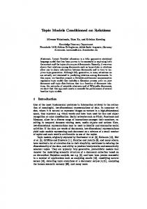
Figure 1. Example of interpretable matrix factorization using probabilistic topic models (A). It allows to represent the data (e.g. documents) as mixtures of only a few topics, which, in turn, can be learned from the data. Illustration of topics learned from text (B) and hyperspectral signatures (C) using probabilistic topic models. The text topics are represented in terms of word clouds containing words with high probabilities. The hyperspectral topics were determined using a wordification approach (C), and represent the spectral characteristics of healthy, diseased, and necrotic parts of leaves.
The work presented here is motivated by the insight that hyperspectral measurements can reveal relationship between the spectral reflectance properties of plants, and their structural characteristics and pigment concentrations, which are considerably influenced by biotic plant stress3,11. This indicates that phenotyping processes can benefit from hyperspectral data analysis and machine learning techniques which can uncover the characteristics of how plants respond to environmental stress. However, since stress reactions result from a complex web of interactions between the genotype and the environment12, common data analysis methods for plant phenotyping such as spectral vegetation indices run the risk of leading to an over-simplified or even misleading interpretation of spectral responses to stress as they consider only few distinct wavelengths. On the other hand, many advanced machine learning techniques extract “factors” or “features” from the data that are not “things” with a “physical” reality13. In turn they are often not easy-to-interpret for non-experts in machine learning. Consequently, next generation plant phenotyping and plant disease detection systems require comprehensive and reliable data analysis methods. In this work, we propose an automated data mining approach that was adopted from the areas of natural language processing and text mining. There, probabilistic topic models have been proven to successfully capture content and underlying hidden topics of document collections and thus to help to organize, search, and understand large amounts of data14. Probabilistic topic model are known to allow for learning meaningful and interpretable representations of massive document collections. As illustrated in Fig. 1(A), given a corpus of text documents, topic models characterize each document using a small number of topics-the clusters. Topics are distributions over words estimated automatically from the documents, where semantically related words have higher probabilities (weights) within a topic. Due to the simple representation as distributions over words, topics are easy to interpret for human analysts. Consider e.g. a subset of Wikipedia articles. Figure 1(B) shows the topics discovered by latent Dirichlet allocation (LDA)15—arguably the most popular probabilistic topic model—represented as word clouds containing the most probable words per topic. As one can see, probabilistic topics indeed result in a meaningful short description; in our case, they are easily interpretable as “Music”, “Color”, or “Education”. Other common approaches for decomposing large data matrices into latent components include principal component analysis (PCA), non-negative matrix factorization (NMF), and archetypal analysis (AA), among others. PCA determines a factorization that retains as much variation in the data as possible16 and is often used for data compression as it reduces noisy and redundant information. NMF17 considers matrices with non-negative entries and results in part-based representation of the data. AA18,19 explains the data in terms of combinations of extreme observations, which are more distinct and hence are more interpretable by human analysts. All these methods implicitly consider a document as a single point in an abstract high dimensional data space. Topic models, in contrast, can provide interpretable representations, which have statistical properties that correspond to those of semantic networks, produced by humans20. Furthermore, although there is a connection between NMF and probabilistic topic modeling21, NMF typically learns more incoherent topics than LDA22. Moreover, the LDA model is easier to explain as it is a generative model: word distributions compromises topics, and a document is drawn from a specific mixture of topics. In turn, the latent components determined by LDA are closer to the probabilistic “topic metaphor” and do not require to reify the “basis vectors” found by NMF. This is essential as the application domain we consider in this work is interdisciplinary and requires scientist with different background to work together. Compared to methods that represent data in terms of extremes or archetypes, LDA can
www.nature.com/scientificreports/ be considered as part-based archetypal analysis. Thus, the topics are extreme distributions in a space spanned by the words in the vocabulary. This view corresponds to the geometric interpretation of LDA as an analysis of data points distributed on a latent simplex15 and, in turn, allows for representing the data as points in the simplex spanned by the topics. Our analysis is based on hyperspectral images of plants in the visible and near infrared ranges. While there are often labels per images such as different genotypes or treatmens of plants, the hyperspectral signatures from single pixels on the images-the focus of our study-are typically not annotated. Hence, it is difficult-if not impossible-to directly employ classification approaches to gain insights into the important hyperspectral characteristics of plant disease progressions4,23. More importantly, the benefit of hyperspectral imaging for plant phenotyping goes beyond the classification of plant stress. Recent studies4,24,25 presented automated analysis pipelines for tracing effects of abiotic and biotic stress to crop plants. Within this context, probabilistic topic models are an intuitive and effective approach for automated, time and cost saving data analysis in order to obtain a deeper understanding of plant pathogen interactions. As we will demonstrate, this exploratory data analysis approach can provide new insights into processes during stress emergence and offers the ability to study how plant physiology is influenced during pathogen infection. In order to extract meaningful topics, i.e. hyperspectral characteristics in terms of important wavelength × reflectance pairs, we propose to “documentify” the hyperspectral images, i.e., we first create “documents” out of hyperspectral signatures. To this end, we “wordify” waveband-energy values as illustrated in Fig. 1(C). Then, we discover hyperspectral characteristics by means of an efficient online approach to regularized LDA. Together, these steps allow one to automatically learn easy-to-interpret representations from large collections of hyperspectral images consisting of millions of pixels/signatures similar to representations used previously to analyze plants suffering from drought26. In other words, this approach provides spectral characteristics of plants affected by various foliar pathogens during the vegetation period. The corresponding topics describe the development of different plant diseases during pathogenesis, allow for an intuitive visualization of information from hyperspectral images, and provide new insights into the dynamics of plant diseases.
Results
In this section, we present and discuss our experimental evaluation on barley plants during development of the foliar diseases powdery mildew, net blotch, and brown rust. The data set considered in this study consists of single barley leaves, recorded every other day after inoculation (dai) with hyperspectral imaging line scanner in the visible and near infrared (400–1000 nm) range4. Each hyperspectral image was represented as dense Λ × N matrix, where N denotes the number of pixels and Λ the number of spectral bands. Stacking all data matrices recorded during pathogenesis into a single matrix resulted in a data matrix with approximately 10 million columns or about 2 billion matrix entries (encoding the reflected energy at different spectral bands). Before determining the topics, we first created sparse matrices out of dense signature × pixel matrices using a wordification approach (see the Methods section). We then ran online regularized LDA for three datasets (for each disease) separately to obtain a set of highly relevant topics related to diseased as well as healthy barley plants. We stopped the online inference when each signature (document) was seen once for each data. Experiments were run on a standard Intel SixCore machine with 3.2 GHz and 16 GB main memory. It took approximately 1.5 hours to determine the topics for each disease dataset where the number of topics was set to K = 25. The Python implementation of online regularized LDA is freely available at https://github.com/mirwaes/sclda.
Topic Labeling. After the models were learned and specific topics for each disease and healthy barley plants
were obtained, we manually annotated the corresponding topics based on information from the literature and their relation to the plant health status. We identified eight classes for net blotch and powdery mildew and six for brown rust. These are visualized in Fig. 2 and summarized in Table 1. Since diseased plants show signs of stress only locally, they also contain examples of topics characteristic for healthy leaves, which can be found in classes 1 and 2 (green boxes) for all diseased plants. Furthermore, regularized LDA can also uncover the specific spectral characteristics at different stages of pathogenesis, as covered by the classes 3–7 for powdery mildew and net blotch, as well as in classes 3–6 for brown rust. In contrast to previous works that considered full signatures to explain the disease progression (cf. Wahabzada et al.4 and references thereine), the topics considered here provide a part based representation covering important wavelength × reflectance pairs. For instance, class 1 has top words (specific wavelength × reflectance) in the range of 550 nm which is highly correlated to the chlorophyll content10,27, the most important pigments in living plants as they are necessary for photosynthesis. The topics which were labeled as diseased in the VIS range (e.g. red and brown boxes in Fig. 2) have top words between 550–700 nm, indicating the disease symptoms such as small necrotic tissue for net blotch, chlorotic spots in early rust development and auburn pustules, and fluffy mycelium and conidia distributed on the upper and lower leaf side for powdery mildew. This caused an overall increase of reflectances which was also observed by28,29 or by30 for Cercospora beticola in sugar beet.
Disease Dynamics. The evaluated topics exhibit a specific location on diseased leaves. Therefore, each topic
could be connected to a specific symptom and the sum of all topics explains the spectral variability within barley leaves. Moreover, localization and probability of topics over time are highly dynamic. This is visualized in Fig. 3(A) for the example of barley leaves infected with powdery mildew 6, 10 and 14 dai (days after inoculation). The first two topics represent the border of a powdery mildew pustule and topic three represents the center of powdery mildew colonies. With further pathogenesis the dominance and probability of the topics change to symptom development. Similar dynamics could be visualized for barley leaves with net blotch and brown rust. This accords with Mahlein et al.30 and Wahabzada et al.4 who previously described hyperspectral dynamics of diseased plants. Scientific Reports | 6:22482 | DOI: 10.1038/srep22482
3
www.nature.com/scientificreports/
Figure 2. Examples of characteristic topics for different classes of plants diseased with powdery mildew, net blotch, and brown rust and topic relevance over time (6, 10 and 14 dai). Each color indicates a different class and a characteristic physiologic process, as summarized in Table 1. This approach visualizes the disease progression and relevant information from hyperspectral images. The size of the text in every second row is proportional to the computed topic relevance. The diseased/necrotic topics become more prominent at later stages, whereas the significance of healthy (green) topics is low.
To compute the disease dynamics quantitatively, we determined the disease progression using the representations learned by regularized LDA. We automatically labeled each pixel i on the image as “diseased”, when the sum of probabilities of labeled diseased topics was greater than a threshold value of ε = 0.25. Then, for each diseased leaf we computed the relative number of diseased/necrotic pixel for 6, 10 and 14 dai. As shown in Fig. 3(B), there is a difference in the amount of affected pixels (= size of infected area on a leaf) for plants inoculated with different diseases. The number of pixels with disease topics is higher for leaves with powdery mildew than for those with other diseases (14 dai). Net blotch and brown rust show similar levels of infestation in the early stages. Brown rust caused tiny chlorotic spots appearing on the tissue, necrosis and loss of water occur only at later stages. Therefore, it has a lower level of colonization than net blotch and powdery mildew in the early stages.
Relative Relevance over Time. In a next step we computed topic relevance at different stages of disease
progression. To assess the age of disease symptoms, it is important to determine how likely it is to observe a particular topic at specific point in time during pathogenesis. Hence, we computed the relevance for a topic k using −1 D Ωkt = ρ kt (t − 1)/∑ ti = 1 ρ ki with ρ k = ∑ d = 1 θdk / D , where t denotes the day after inoculation and θd is the topics representation of a document d. Note that we do not measure the appearance of the topics per pixel, as it was done in the previous section, but the relative increase in probability for each topic compared to the previous days. The word clouds in Fig. 2 show the results with respect to the increase in topic relevance 6, 10 and 14 dai. Here, the size of the text is proportional to the computed values Ωkt. The diseased/necrotic topics become more prominent at later stages, whereas the significance of healthy (green) topics is low. The diseased/necrotic topics for powdery mildew in Fig. 2(A) have higher importance starting at day 6 after inoculation. This can be explained by the high amount of white mycelial colonies on the the relatively intact tissue that caused a high number of conidia produced4. Net blotch, on the other hand, showed early chlorosis and necrosis, causing structural and biochemical changes and necrotic tissue damage, as covered by the relevances in Fig. 2(B). Brown rust showed comparatively minor impact on barley tissue in early stages, which can be also deduced from Fig. 2(C). First chloroses appeared around 7 dai causing an increase of the relevance of topics covering structural changes and pustule border. However, rust spores started to rupture the epidermis 10 dai, causing an increase in importance of topics related to sporulation. Scientific Reports | 6:22482 | DOI: 10.1038/srep22482
4
www.nature.com/scientificreports/
Disease
Class
Net blotch Pyrenophora teres
Brown rust Puccinia hordei
Relevant functional spectral range
Literature
Description and symptom apparance
27,43,44
green, healthy leaf tissue with high pigment absorbance
700–1000 nm
45,46
healthy tissue with moderate backscattering
500–650 nm
27,44,47
beginning chlorosis, outer border of pustules
700–1000 nm
45,48,49
mycelium growth and development of conidiophore and conidia causing increased backscattering
healthy VIS
400–700 nm, partly 700–1000 nm
2
healthy NIR
3
pigment degradation VIS
4
structural changes NIR
1
Powdery mildew Blumeria graminis hordei
Label
5
pustule border
560–700 nm
47
6
pustule
560–700 nm
10,27,44
browning, inner border pustules
7
beginning necrosis
500–680 nm
47
beginning necrosis at pustule sites, center pustules
8
high blue reflection
400–450 nm
50
powdery mildew mycelium, conidiophores and conidia
1
healthy VIS
400–700 nm, partly 700–1000 nm
27,43,44
green, healthy leaf tissue with high pigment absorbance
2
healthy NIR
700–1000 nm
45,46
3
chlorosis VIS
500–580 nm, 550 nm, 700 nm
27,44,47
4
structural changes NIR
700–1000 nm
45,48
5
browning
580–700 nm
47
net-like symptom development
6
beginning necrosis
580–700 nm
51
inner parts of the symptoms with characteristic net-like necrosis
7
necrosis
450-700 nm, 680 nm
47
tissue damage and drying causing shift of the red edge
8
high blue reflection
400–500 nm
50
increased blue reflection
2
healthy VIS
400–700 nm partly 700–1000 nm
27,34,52
1
healthy NIR
700–1000 nm
45,50
high VIS reflectance / shift green peak
healthy tissue with moderate NIR reflectance pigment degradation and chlorosis at symptom sites beginning tissue damage
green, healthy leaf tissue with high pigment absorbance healthy tissue with moderate NIR reflectance
4
chlorosis VIS
550–650 nm
43,44,53
3
structural changes NIR
700–1000 nm
45,48
chlorotic halos around rust pustules
5
pustule border
550–650 nm
43
first uredospores appear, inner border pustules
6
sporulation
600–710 nm
43
uredospores appear at the center of rust pustules, advanced senescence
increased NIR plateu caused by ruptured epidermis and tissue damage
Table 1. Relevant spectral topics and corresponding biochemical labels in the visble and near-infrared range.
Discussion
We present an automated, data-driven pipeline for extracting characteristic spectral regions of plants, infected by foliar pathogens. Effective analysis and interpretation of hyperspectral imaging data are still limiting factors for an implementation of sensor technologies into plant phenotyping or precision agriculture31,32. Probabilistic topic models, originating from text mining, were successfully adopted to analyze hyperspectral images of plants. Based on the proposed pipeline, it is possible to uncover the hyperspectral language of plant diseases, to visualize characteristic topics during symptom development, and to monitor disease progress. Detecting and utilizing information of the electromagnetic spectrum of plants, infected with pathogens, one can observe disease development during pathogenesis33. The proposed pipeline strikes a new path for plant phenotyping and characterization of early processes during pathogenesis by optical sensors. The word clouds, shown in Fig. 2, are an example of an interpretable summary of high dimensional data, elucidating processes and key aspects of pathogenesis. Compared to common data analysis approaches, multiple benefits are present. In contrast to vegetation indices, which are a correlated to biophysical plant parameters and are not disease specific27,34, the entire spectral information is utilized effectively. Wavelet analysis, which outperformed a range of spectral vegetation indices in a predictive model for chlorophyll content35, aims to provide meaningful quantitative information, but would hardly be capable to gather the entire complexity of up- and down regulated parameters during plant disease development. Classification methods such as Support Vector Machines or Artificial Neural Networks aim at differentiating among classes such as healthy or diseased plant tissue23,32. Here the results highly depend on the choice of features from hyperspectral images and could be a complementary methodology to our proposed probabilistic topic models, avoiding time intensive and error prone human labelling. The hyperspectral language of plants assessed with the wordification approach corresponds to the phenotype of diseased plants and enables a highly accurate description of disease progression over time and in space. They result in hyperspectral topics that conform to plant physiological knowledge, allowing to characterize plant pathogen interactions. This is demonstrated in Fig. 2 and Table 1, showing the relevant hyperspectral topics and Scientific Reports | 6:22482 | DOI: 10.1038/srep22482
5
www.nature.com/scientificreports/
Figure 3. Localisation and dynamic of relevant topics of a barley leave diseased with powdery mildew at 6, 10 and 14 dai (A). Spatial and temporal dynamics of the topics are in accordance to the symptom development. Disease quantification based on disease specific topics 6, 10 and 14 days after inoculation (B). It exhibits a high sensitivity for disease detection and quantification.
corresponding biochemical labels. A comparison of latent components found by different data mining methods from a hyperspectral image of a diseased plant is shown in Supplementary Fig. S1(A). Principal components obtained by PCA, for instance, can reveal the variations existing in the data, but the corresponding intensities are abstract values that make statistically sense, but they do not have a physical meaning. Other methods, such as NMF or simplex volume maximization19 (SiVM, a fast method for archetypal analysis), find components that are corrupted by noise or can not represent important parts of hyperspectral signature. The wordification approach, on the other hand, extracts latent part-based components that contain the reflectance intensities at different wavelengths, as shown in Fig. 2 and summarized in Table 1. They can be interpreted easily by domain experts. A comparison to a standard approach for topic models without regularization has revealed that the topics found by non-regularized LDA, shown in Supplementary Fig. 1(B), are not coherent. Furthermore, they are dominated by topics with lower reflectance intensities, which represent the healthy part of the leaf, while ignoring the variations of diseased spectra. This is another justification for the proposed fast regularized LDA, as it considers the short-range dependencies of hyperspectral words and produces coherent topics that can be associated with different leaf disease stages. The hyperspectral topics and the resulting word clouds visualizes the underlying biophysical and biochemical processes during disease development. The identified topics belong to specific regions of disease different symptoms or/and to specific developmental phases. This aspect is in accordance to30,36, who found characteristic spectral signatures for symptoms of Cercospora leaf spot of sugar beet, in time and space. The prominence of a specific trait or developmental phase can be visualized intuitively by the presented wordification approach. Powdery mildew diseased tissue is covered by white mycelium colonies producing an increasing amount of conidia. Besides a development of characteristic powdery pustules, accompanying chlorosis can be read from the topic models. Net blotch and rust share the occurrence of chlorosis in early stages of disease development. Besides, net blotch causes early necrosis. Due to this specific necrotrophic aspect, topics, correlated to pigment degradation, water loss and cellular tissue damage are characteristic for net blotch infestation. As a biotrophic fungi, P. hordei, the causal agent of rust disease has a moderate influence into the host plant biophysiology. The relation among healthy and diseased tissue is well-balanced over time, sporulation specific topics appear at later time points. These observation are in accordance to hyperspectral dynamics of barley diseases visualized as single sketches and metro maps of plant diseases by4. Our work provides several interesting avenues for future work. Next to experiments under field conditions, one should aim at even further improving the topic quality, for instance, by applying hierarchical, (semi-) supervised and relational versions of topic modeling. The models may be used to identify the most relevant time when biologists have to gather samples for invasive, molecular examinations. Active LDA approaches could be employed to speed up computations even further. This would also allow to discard documents or signatures during learning, or to determine those which are most specific for a particular disease at different points in time. One should also move from the unsupervised setting considered here to the supervised setting, for example, for classifying disease-specific spectra at different stages of pathogenesis. One approach to do so would be to train, say, a Support Vector Machine for each measurement day using our low-dimensional topic representation. A more sophisticated approach would be to adapt a temporal classifier, say, a Conditional Random Field, or to even smooth the embeddings over time using Dirichlet Multinomial Regression37. Ultimately, one should start developing joint models that compute low-dimensional embeddings via topics and classifications over time. This is a form of (semi)-supervised LDA, and the present work paves the way to do so. Overall, the proposed approach will support upcoming sensor applications for phenotyping tasks like, for instance, the screening of disease resistant genotypes or precision agriculture applications for the localization of primary disease foci in fields1,3,33.
Methods
Plant material and plant pathogens. Analysis was done on a dataset recorded from barley plants
which were grown in a controlled greenhouse environment and were used for hyperspectral measurements after
www.nature.com/scientificreports/ reaching growth stage 32. A detailed description of the plant material and pathogens can be found in Wahabzada et al.4. The plants were inoculated with different fungal pathogens, namely, Pyrenophora teres (causing net blotch), Puccinia hordei (causing leaf rust of barley), and Blumeria graminis hordei (causing powdery mildew). A control group was kept non-inoculated. Hyperspectral images were recorded 4, 6, 8, 10, 12, 14 days after inoculation (dai) with an ImSpector V10E, which covers the visible and near-infrared (400–1000 nm) range. The camera has a spectral resolution of 2.8 nm and a spatial resolution of 0.12 mm per pixel, and results in 210 hyperspectral bands. The Savitzky-Golay filter38 was applied to remove noise and to smooth the hyperspectral signature information.
Wordification. We are interested in finding characteristic patterns in the combination of reflectance val-
ues at specific wavelength. To this end, we employ probabilistic topic models which require input in terms of sparse data matrices. We therefore apply wordification to given hyperspectral images. In particular, we propose to discretize hyperspectral signatures as follows: we decompose the space covering the full signatures into R possible reflectance words. Since reflectance values are normalized they range from 0 and 1 and thus facilitate this decomposition. Accordingly, in a signature each wavelength can consist of one of the R distinct reflectance words, which results in a total number of Λ × R different possible spectral words. This process is illustrated in Fig. 1(B) and detailed in Supplementary Fig. S2(A). It shows an example of a hyperspectral image where each pixel is represented by a signature. After wordification, each document (signature) is represented by Λ out of Λ × R possible spectral words. The benefits of this approach are that it is fast to compute, does not require additional efforts to construct a dictionary, and yields interpretable results since each word correspond to a specific wavelength-reflectance pair. The use of discretized values instead of continuous ones is further motivated by the fact that, according to plant physiologist, small difference in reflectance values are of minor importance. Nevertheless, since signatures are still curves over spectral bands, we also take the short-range dependencies of words into account. For that we compute a word-dependency matrix C, cf. Supplementary Fig. S2(B), that is created using pointwise mutual information (PMI). PMI as the measure of word association is defined as follows39: PMI (w i , w j ) = log
P (w i , w j ) P (w i ) P (w j )
.
(1)
In order to also capture co-occurrences between different reflectances within a wavelength, we proceed as follows: we first aggregate the signatures in the images into non-overlapping squares of 5 × 5 pixels. Spectral word co-occurrences are computed using a sliding window of stride length 1 in each direction (wavelength and reflectance) in the aggregated signatures. Next, given the document-word representation of signatures and their short-range dependencies, we are ready to apply regularized topic models. For our experiments on hyperspectral images of diseased plants, we transformed each signature into document representation by setting R = 50, before running the topic models. We computed the PMI only for the words with minimum appearance of Nw = 250 and only kept the positive values.
Regularized Probabilistic Topic Models. LDA, as proposed by Blei et al.15, is a Bayesian probabilistic
model that describes a generative process of how words in documents might be generated on the basis of latent topics. Fitting an LDA topic model given a set of training documents requires approximate inference techniques that are computationally expensive. For instance, in variational Bayesian (VB) inference, the true posterior is approximated using a simpler, fully factorized distribution q. For that, following15,40, we choose q(z, θ, β) of the form q (z di = k) = φdw dik, q (θd ) = Dir (θd , γ d), and q (β k) = Dir (β k, λk). The variational parameters φ, γ, and λ are optimized to maximize the Evidence Lower BOund (ELBO) log p (w α , η) ≥ L (w , φ, γ , λ) q [log p (w , z , θ , β α , η)] − q [log q (z , θ , β )],
(2)
which is equivalent to minimizing the Kullback-Leibler divergence between q(z, θ, β) and the true posterior p (z , θ , β w , α , η). For introducing a structured prior to regularize the word-topic probabilities, one can build on top of the recent regularized Gibbs approach due to39, who have demonstrated that regularization improves the topic coherence. Before presenting a scalable online approach for regularized LDA, we present a variational Bayes inference for the batch case.
Variational Bayes Inference for Regularized LDA. For regularized LDA, we view each topic as a mixture of word probabilities given by the word-pair dependency matrix C (a W × W matrix, where W denotes the size of vocabulary and Cij ≥ 0), that is β k ∝ Cbk where bk ∼ Dir (η).
(3)
In VB, the true posterior is approximated using fully factorized distributions q. Consequently, we parameterize the word probabilities b by introducing a new variational parameter v, i.e. q (bk ) = Dir (bk , ν k). The per-word topic assignments z are parameterized by φ, and the posterior over the per-document topic weights θ are parameterized by γ, as for the standard LDA. The part of the likelihood including the specific parameter v can then be written as
L[ν ] = q [log p (w z , C , b)] + q [log p (b η)] − q [log q (b)]
(4)
and the remaining part of the ELBO remains unchanged. To approximate the first term of Eq. (4), we adapt the lower bound on the log-sum-exp function41, q [log ∑i X i ] ≥ log ∑i exp(q [log X i ]) (for a detailed proof see e.g.42) to our case, which follows by applying Jensen’s inequality: q [log p (w z = k , C , b)] = ≥
W
W
i
j
∑Φik q log ∑C ijb jk W
∑Φik log ∑ exp (q [log C ijb jk ]) i
=
j
W
∑Φik log ∑C ij exp (q [log b jk ]), i
(5)
j
D W where ∑W w Φwk = ∑ d ∑ w φdwk. This is still a lower bound, so maximizing it will improve the ELBO. The expectation of logb under the distribution q is: q [log bwk ] = Ψ (ν wk) − Ψ (∑s ν sk) , where Ψ denotes digamma function, the first derivative of logΓ (the logarithm of the gamma function). The remaining terms of the Eq. (4) (for a topic k) are
To derive a VB approach, we compute the derivative of Eq. (4) with respect to the variational parameter vwk. After applying the chain rule and rearranging terms, this gives ∂q [log p (w z , C , b)]/∂ν wk W
= Ψ1(ν wk) ∑ Φik i
C iw exp (q [log bik ])
∑W j C ij
W − Ψ1∑ v sk ∑ Φik i exp (q [log b jk ]) s
(8)
for the first term of Eq. (4). Taking the derivatives for all terms together we arrive at: W C iw exp (q [log bik ]) + η − ν wk ∂L /∂ν wk = Ψ1(ν wk) ∑ Φik W i ∑ j C ij exp (q log b jk ]) W W − Ψ1∑ ν sk ∑ (Φik + η − ν ik). i s
(9)
Setting the above derivative to zero, we obtain the following fixed point update: ν wk = η +
W
∑ Φik i
C iw exp (q [log bik ])
∑W j C ij exp (q [log b jk ])
.
(10)
This is a proper generalization of the standard VB approach. To see this, we simply set the word-pair dependency matrix C to the identity matrix. It then follows that ν wk = η +
∑ ndw φdwk. d
(11)
To derive a learning algorithm, i.e. to actually optimize L, we follow a coordinate ascent on the variational parameters φ, γ and v. Given the word topic probabilities β from Eq. (3), this yields the following per-document updates for φ and γ in the E-step: φdwk ∝ β wk ∗ exp (q [log θdk ]), γ dk = α +
(12)
W
∑ ndw φdwk. w
(13)
In the M-step, we perform fixed point updates as in Eq. (10) and compute the values βwk using Eq. (3) as follows:
Figure 4. Online variational Bayes for regularized latent Dirichlet allocation.
β wk ∝
W
W
i
∑ C iw exp Ψ (ν ik) − Ψ ∑ν sk . s
(14)
However, recall that one of our main goals is the application of regularized VB to hyperspectral images of plants. Since a single image can already consist of hundreds of thousands of signatures (documents) so that several images (as in the case of our experiments) easily scale to several million documents, batch VB is likely to be infeasible in terms of running time. Consequently, we will develop an online variant of regularized VB that scales well to massive datasets.
Online Variational Bayes Inference for Regularized LDA. Since setting the word-dependency matrix
C to identity matrix results in standard VB, it is intuitively clear that we may extend the regularized VB to the online case by adapting online variational Bayes40. Specifically, the variational lower bound for the regularized VB can be written as L =
D
∑ {q [log p (wd θd , z d, C , b)] + q [log p (z d θd )] d
− q [log q (z d)] + q [log p (θd α)] − q [log q (θd )] + (q [log p (b η)] − q [log q (b)])/D}
D
∑ (nd , φd, γ d, C, ν), d
(15)
where (nd , φd, γ d, C , ν) is the dth document’s contribution to the variational bound. The per-corpus terms are summed together and divided by the number of documents D. This allows us to derive the online approach since the optimal v is the one for which L maximized after fitting the per-document parameter. In other words, we can use the regularized updates in a per-document manner as summarized in Fig. 4. ˜ . Then, an The algorithm first randomly selects documents from the entire dataset by forming a mini-batch D E-step is performed to find locally optimal values of γ and φ while holding β fix. In the M-step, several fixed point updates for ν are computed using νwk =
W C iw exp (q [log bik ]) D φdik +η ∑ ∑ ∑ j C ij exp (q [log b jk ]) S d∈ D˜ i
(16)
˜ (currently observed mini-batch), where we re-scale by D given the document-specific parameter φd with d ∈ D S to update as though we would have seen all documents. Multiple documents are used per update to reduce variance. The parameter ν is updated through a weighted average of its previous value, and ν (computed for the current mini-batch using fixed point updates as in Eq. (16)). Furthermore, new values of β are computed given ν and word-dependency matrix C. The rate of change ρ t is set to ρ t (τ 0 + t )−κ with κ ∈ (0.5, 1] in order to guarantee convergence. Note that, as in the non-regularized case, when setting the batch size to S = D and κ = 0 we recover regularized batch VB. Scientific Reports | 6:22482 | DOI: 10.1038/srep22482
9
www.nature.com/scientificreports/
References
1. Walter, A., Liebisch, F. & Hund, A. Plant phenotyping: from bean weighing to image analysis. Plant Methods 11, 1–11 (2015). 2. Fiorani, F. & Schurr, U. Future scenarios for plant phenotyping. Annu. Rev. Plant Biol. 64, 267–291 (2013). 3. Mahlein, A.-K. Plant disease detection by imaging sensors–parallels and specific demands for precision agriculture and plant phenotyping. Plant Dis, 100, 241–251 (2016). 4. Wahabzada, M. et al. Metro maps of plant disease dynamics–automated mining of differences using hyperspectral images. PLOS One 10, e0116902 (2015). 5. Walters, D. et al. Control of foliar diseases in barley: Towards an integrated approach. Eur. J. of Plant Pathol. 133, 33–73 (2012). 6. Furbank, R. T. & Tester, M. Phenomics-technologies to relieve the phenotyping bottleneck. Trends Plant Sci. 16, 635–644 (2011). 7. Mahlein, A.-K., Oerke, E.-C., Steiner, U. & Dehne, H.-W. Recent advances in sensing plant diseases for precision crop protection. Eur. J. of Plant Pathol. 133, 197–209 (2012). 8. Rascher, U. et al. Non-invasive approaches for phenotyping of enhanced performance traits in bean. Funct. Plant Biol. 38, 968–983 (2011). 9. Curran, P., Dungan, J. & Gholz, H. Exploring the relationship between reflectance red edge and chlorophyll content in slash pine. Tree Physiol. 7, 33–48 (1990). 10. Gitelson, A. & Merzlyak, M. Signature analysis of leaf reflectance spectra: algorithm development for remote sensing of chlorophyll. Plant Physiol. 148, 494–500 (1996). 11. Govender, M., Dye, P. J. , Weiersbye, I. M., Witkowski, E. T. F. & Ahmed, F. Review of commonly used remote sensing and groundbased technologies to measure plant water stress. Water SA 35, 741–752 (2009). 12. Houle, D., Govindaraju, D. R. & Omholt, S. Phenomics: the next challenge. Nat. Rev. Genet. 11, 855–866 (2010). 13. Mahoney, M. & Drineas, P. CUR matrix decompositions for improved data analysis. Proc. Natl. A. Sci. 106, 697–702 (2009). 14. Blei, D. M. Probabilistic topic models. Commun. ACM 55, 77–84 (2012). 15. Blei, D., Ng, A. & Jordan, M. Latent dirichlet allocation. J. Mach. Learn. Res. 3 , 993–1022 (2003). 16. Jolliffe, I. T. Principal Component Analysis, 1–9 (Springer-Verlag New York, 2002) 2nd edn. 17. Lee, D. D. & Seung, H. S. Learning the parts of objects by non-negative matrix factorization. Nature 6755, 788–799 (1999). 18. Cutler, A. & Breiman, L. Archetypal analysis. Technometrics 36, 338–347 (1994). 19. Thurau, C., Kersting, K., Wahabzada, M. & Bauckhage, C. Descriptive matrix factorization for sustainability: Adopting the principle of opposites. Data Min. Knowl. Disc. 24, 325–354 (2012). 20. Griffiths, T. & Steyvers, M. A probabilistic approach to semantic representation. In Gray, W. D. & Schunn, C. (eds) Proceedings of the 24th Annual Conference of the Cognitive Science Society, Fairfax, Virginia, USA, 381–386 (Lawrence Erlbaum Associates, Inc. 2002). 21. Ding, C., Li, T. & Peng, W. On the equivalence between non-negative matrix factorization and probabilistic latent semantic indexing. Comput. Stat. Data An. 52, 3913–3927 (2008). 22. Stevens, K., Kegelmeyer, P., Andrzejewski, D. & Buttler, D. Exploring topic coherence over many models and many topics. In Proceedings of the 2012 Joint Conference on Empirical Methods in Natural Language Processing and Computational Natural Language Learning, Jeju Island, Korea, 952–961 (Association for Computational Linguistics, 2012). 23. Moshou, D. et al. Plant disease detection based on data fusion of hyper-spectral and multi-spectral fluorescence imaging using kohonen maps. Real-Time Imaging 11, 75–83 (2005). 24. Kuska, M. et al. Hyperspectral phenotyping on the microscopic scale: towards automated characterization of plant-pathogen interactions. Plant Methods 11, 28 (2015). 25. Römer, C. et al. Early drought stress detection in cereals: Simplex volume maximization for hyperspectral image analysis. Funct. Plant Biol. 39, 878–890 (2012). 26. Wahabzada, M. et al. Latent dirichlet allocation uncovers spectral characteristics of drought stressed plants. In de N. Freitas, K. M. (ed.) Proceedings of the 28th Conference on Uncertainty in Artificial Intelligence, Catalina Island, California, USA, 852–862 (AUAI Press, 2012). 27. Blackburn, G. A. Hyperspectral remote sensing of plant pigments. J. Exp. Bot. 58, 844–867 (2007). 28. Teng, P. & Close, R. Spectral reflectance of healthy and leaf rust-infected barley leaves. Aust. Plant Pathol. Soc. Newsl. 6, 7–9 (1977). 29. Lorenzen, B. & Jensen, A. Changes in leaf spectral properties induced in barley by cereal powdery mildew. Remote Sens. Environ. 27, 201–209 (1989). 30. Mahlein, A.-K., Steiner, U., Hillnhutter, C., Dehne, H.-W. & Oerke, E.-C. Hyperspectral imaging for small-scale analysis of symptoms caused by different sugar beet diseases. Plant Methods 8, 3 (2012). 31. Li, L., Zhang, Q. & Huang, D. A review of imaging techniques for plant phenotyping. Sensors 14, 20078–20111 (2014). 32. Behmann, J., Mahlein, A.-K., Rumpf, T., Römer, C. & Plümer, L. A review of advanced machine learning methods for the detection of biotic stress in precision crop protection. Precis. Agric. 16, 239–260 (2015). 33. Mutka, A. & Bart, R. Image-based phenotyping of plant disease symptoms. Front. Plant Sci. 5, doi: 10.3389/fpls.2014.00734 (2015). 34. Gitelson, A. A., Gritz, Y. & Merzylak, M. N. Relationships between leaf chlorophyll content and spectral reflectance and algorithms for non-destructive chlorophyll assessment in higher plant leaves. J. Plant Physiol. 160, 271–282 (2003). 35. Blackburn, G. A. & Ferwerda, J. G. Retrieval of chlorophyll concentration from leaf reflectance spectra using wavelet analysis. Remote Sens. Environ. 112, 1614–1632 (2008). 36. Leucker, M., Mahlein, A.-K., Steiner, U. & Oerke, E.-C. Improvement of lesion phenotyping in Cercospora beticola–sugar beet interaction by hyperspectral imaging. Phytopathology, 106, 177–184 (2016). 37. Kersting, K. et al. Pre-symptomatic prediction of plant drought stress using dirichlet-aggregation regression on hyperspectral images. In Hoffmann, J. and Selman, B. (ed.) Proceedings of the Twenty-Sixth AAAI Conference on Artificial Intelligence, Toronto, Ontario, Canada, 302–308 (AAAI Press, 2012). 38. Savitzky, A. & Golay, J. Smoothing and differentiation of data by simplified least squares procedures. Anal. Chem. 36(8), 1627–1639 (1964). 39. Newman, D. , Bonilla, E. V. & Buntine, W. Improving topic coherence with regularized topic models. In Shawe-Taylor, J., Zemel, R., Bartlett, P., Pereira, F. & Weinberger, K. (eds.) Proceedings of the 25th Annual Conference on Neural Information Processing Systems, Granada, Spain, 496–504 (Curran Associates, Inc. 2011). 40. Hoffman, M., Bach, F. R. & Blei, D. M. Online learning for latent dirichlet allocation. In Lafferty, J., Williams, C., Shawe-Taylor, J., Zemel, R. & Culotta, A. (eds) Proceedings of the 24th Annual Conference on Neural Information Processing Systems, Vancouver, British Columbia, Canada, 856–864 (Curran Associates, Inc. 2010). 41. Boyd, S. & Vandenberghe, L. Convex Optimization page 72 (Cambridge University Press, 2004). 42. Paisley, J. Two useful bounds for variational inference. Techical Repport (2010). Available at: http://www.columbia.edu/ jwp2128/ Teaching/E6892/papers/twobounds.pdf (November 30, 2015). 43. Gitelson, A. A. & Merzlyak, M. N. Spectral reflectance changes associate with autumn senescence of Aesculus hippocastanum L. and Acer platanoides L. leaves. Spectral features and relation to chlorophyll estimation. J. Plant Physiol. 143, 286–292 (1994). 44. Gamon, J. A. & Surfus, J. S. Assessing leaf pigment content and activity with a reflectometer. New Phytol. 143, 105–117 (1999). 45. Penuelas, J. & Filella, I. Visible and near-infrared reflectance techniques for diagnosing plant physiological status. Trends Plant Sci. 3, 151–156 (1998). 46. Carter, G. A. & Miller, R. L. Early detection of plant stress by digital imaging with narrow stress-sensitive wavebands. Remote Sens. Environ. 50, 295–302 (1994).
www.nature.com/scientificreports/ 47. Merzlyak, M. N., Gitelson, A. A., Chivkunova, O. B. & Rakitin, V. Y. Non-destructive optical detection of pigment changes during leaf senescence and fruit ripening. Physiol. Plantarum 106, 135–141 (1999). 48. Jensen, J. R. Remote Sensing of the Environment–An Earth Resource Perspective 355–408 (Pearson Prentice Hall, 2002) 2nd edn. 49. Jacquemoud, S. & Ustin, L. S. Leaf optical properties: a state of the art. In 8th International Symposium of Physical Measurements & Signatures in Remote Sensing 223–332 (CNES, 2001). 50. Carter, G. A. & Knapp, A. K. Leaf optical properties in higher plants: linking spectral characteristics to stress and chlorophyll concentration. Am. J. Bot. 88, 677–684 (2001). 51. Horler, D. N. H., Dockray, M. & Barber, J. The red edge of plant leaf reflectance. Int. J. Remote Sens. 4, 273–288 (1983). 52. Sims, D. A. & Gamon, J. A. Relationship between leaf pigment content and spectral reflectance across a wide range of species, leaf structures and developmental stages. Remote Sens. Environ. 81, 337–354 (2002). 53. Blackburn, G. A. Spectral indices for estimating photosynthetic pigment concentrations: a test using senescent tree leaves. Int. J. Remote Sens. 19, 657–675 (1998).
Acknowledgements
This work could be carried out due to the financial support of the German Federal Ministry of Education and Research (BMBF) within the scope of the competitive grants program “Networks of excellence in agricultural and nutrition research–CROP.SENSe.net (Funding code: 0315529), junior research group” Hyperspectral phenotyping of resistance reactions of barley.
Author Contributions
Conceived and designed the experiments: M.W., A.K.M., C.B., U.S., E.C.O. and K.K. Performed the experiments: M.W. and A.K.M. Analyzed the data: M.W., A.K.M. and K.K. Contributed reagents/materials/analysis tools: M.W., A.K.M., C.B., U.S., E.C.O. and K.K. Wrote the paper: M.W., A.K.M., C.B. and K.K. All authors reviewed the manuscript.
Additional Information
Supplementary information accompanies this paper at http://www.nature.com/srep Competing financial interests: The authors declare no competing financial interests. How to cite this article: Wahabzada, M. et al. Plant Phenotyping using Probabilistic Topic Models: Uncovering the Hyperspectral Language of Plants. Sci. Rep. 6, 22482; doi: 10.1038/srep22482 (2016). This work is licensed under a Creative Commons Attribution 4.0 International License. The images or other third party material in this article are included in the article’s Creative Commons license, unless indicated otherwise in the credit line; if the material is not included under the Creative Commons license, users will need to obtain permission from the license holder to reproduce the material. To view a copy of this license, visit http://creativecommons.org/licenses/by/4.0/