Platform-Specific Code Generation from Platform ... - ScholarlyCommons

University of Pennsylvania

ScholarlyCommons Departmental Papers (CIS)

Department of Computer & Information Science

12-2015

Platform-Specific Code Generation from PlatformIndependent Timed Models BaekGyu Kim University of Pennsylvania, [email protected]

Lu Feng University of Pennsylvania, [email protected]

Oleg Sokolsky University of Pennsylvania, [email protected]

Insup Lee University of Pennsylvania, [email protected]

Follow this and additional works at: http://repository.upenn.edu/cis_papers Part of the Computer Engineering Commons, and the Computer Sciences Commons Recommended Citation BaekGyu Kim, Lu Feng, Oleg Sokolsky, and Insup Lee, "Platform-Specific Code Generation from Platform-Independent Timed Models", IEEE Real-Time Systems Symposium (RTSS 2015) . December 2015.

IEEE Real-Time Systems Symposium (RTSS 2015). San Antonio, Texas, U.S.A., Dec 2015. This paper is posted at ScholarlyCommons. http://repository.upenn.edu/cis_papers/795 For more information, please contact [email protected].

Platform-Specific Code Generation from Platform-Independent Timed Models Abstract

Many safety-critical real-time embedded systems need to meet stringent timing constraints such as preserving delay bounds between input and output events. In model-based development, a system is often implemented by using a code generator to automatically generate source code from system models, and integrating the generated source code with a platform. It is challenging to guarantee that the implemented systems preserve required timing constraints, because the timed behavior of the source code and the platform is closely intertwined. In this paper, we address this challenge by proposing a model transformation approach for the code generation. Our approach compensates the platform-processing delays by adjusting the timing parameters in system models, based on an Integer Linear Programming problem formulation. We demonstrate the usefulness of our approach via a case study of infusion pump systems. Experimental results show that the code generated using our approach can better preserve the timing constraints. Disciplines

Computer Engineering | Computer Sciences Comments

IEEE Real-Time Systems Symposium (RTSS 2015). San Antonio, Texas, U.S.A., Dec 2015.

This conference paper is available at ScholarlyCommons: http://repository.upenn.edu/cis_papers/795

Platform-Specific Code Generation from Platform-Independent Timed Models BaekGyu Kim1,2

Lu Feng1

Oleg Sokolsky1

Insup Lee1

1 University 2 Toyota

of Pennsylvania InfoTechnology Center, U.S.A.

Abstract—Many safety-critical real-time embedded systems need to meet stringent timing constraints such as preserving delay bounds between input and output events. In model-based development, a system is often implemented by using a code generator to automatically generate source code from system models, and integrating the generated source code with a platform. It is challenging to guarantee that the implemented systems preserve required timing constraints, because the timed behavior of the source code and the platform is closely intertwined. In this paper, we address this challenge by proposing a model transformation approach for the code generation. Our approach compensates the platform-processing delays by adjusting the timing parameters in system models, based on an Integer Linear Programming problem formulation. We demonstrate the usefulness of our approach via a case study of infusion pump systems. Experimental results show that the code generated using our approach can better preserve the timing constraints.

I. I NTRODUCTION Many safety-critical real-time embedded systems need to meet stringent timing constraints, of which a common type is the bounded delay between input and output events. For example, a car should stop (output event) within three seconds when a driver hits a brake (input event); a pacemaker should generate electrical signals (output event) within eight milliseconds when an abnormal heart rhythm is detected (input event). The violation of such timing constraints may lead to catastrophic consequences. Thus, it is important to guarantee that the developed real-time embedded systems satisfy the timing constraints. One promising approach is via modelbased development. First, a system model is built to capture abstractions of the system’s timed behavior. Then, if the model is verified to satisfy the timing constraints, source code is automatically generated from the model using a code generator. Finally, the generated code is implemented on a platform. By platform, we refer to a collection of hardware (e.g., sensors/actuators) and software (e.g., real-time operating systems and I/O device drivers) that are required for the code to read input from or write output to the environment. System models are typically constructed independently of a specific platform for a few benefits: (1) the generated source code can be implemented on many different platforms, and (2) the modeling process can be initiated without knowledge of specific platform in the early system development stage. Stateof-the-art code generators, such as Real-Time Workshop [13] and TIMES [4], produce source code using timing parameters specified in a system model directly, with the assumption that the input/output (I/O) communication between the code and the environment can be processed infinitely fast by a platform. *This research was supported in part by NSF CNS-1035715 and the DGIST Research and Development Program of the Ministry of Science, ICT and Future Planning of Korea (CPS Global Center). *This work has been performed while the first author was at the University of Pennsylvania.

However, it is difficult, if not impossible, for any platform to meet this assumption in practice, due to processing delays caused by, e.g., I/O device drivers or communication jitter. In our previous work, we proposed to overcome this obstacle by modeling architectural aspects of platforms [12] [10] and generating test cases [11]. However, one limitation is that, the code generated from models that incorporate platformprocessing delays, when being implemented on a specific platform, may yield a system that does not respect timing constraints verified at the modeling level. Because platformprocessing delays are added to the code-level delays. It is challenging to guarantee that the implemented systems preserve required timing constraints, because timing aspects of the system model, the code and the platform are closely intertwined. In this paper, we aim to address this challenge by proposing a model transformation approach for the code generation. We argue that system models are not appropriate representations of the code-level timed behavior. We transform a system model into a software model by explicitly characterizing (non-zero) platform-processing delays and appropriately compensating those delays. The software model is then used to generate code, which would be implemented on the platform whose processing delays are compensated during the model transformation process. The resulting system implementation is guaranteed to meet the timing constraints that have been verified in the system model. We restrict our attention to timing constraints in the type of bounded delay between I/O events. Our model transformation approach involves two steps. First, check whether it is feasible to compensate the processing delays of a given platform while preserving bounds on delays between observable events in the system model and implementation. Second, adjust timing parameters in the system model to obtain a software model that compensates the platform-processing delays. We formulate and solve the problem using Integer Linear Programming (ILP). We define the objective function of ILP based on the goal of obtaining a software model with the least timed behavior perturbation from the system model. The linear constraints of ILP are given to quantify the delay-bound differences between the system model and implementation, taking into account the model’s I/O delays accumulated over paths (between pairs of I/O transitions) and the platform-processing delays. By solving the ILP problem, we obtain a set of timing parameter assignments that can be used to transform the system model into a software model. We demonstrate the usefulness of our approach via a case study of infusion pump systems. Experimental results show that systems implemented with the code generated from our transformed software models have (significantly) better performance in terms of timing constraints preservation. The rest of this paper is organized as follows. Section II

a1?

L1 1

Fig. 1.

[t1l , t1u ]

L2

a2! xa1  2  xa1  10

2

[t2l , t2u ]

L3

a3? xa2  7  xa2  10

3

L4

[t3l , t3u ]

Model 1 with variable assignment (Sequential Pattern)

introduces a motivating example, the problem statement and an overview of our approach. Section III describes how to compute the minimum and maximum delays of I/O events in the system model and implementation. Section IV develops the ILP problem formulation for the model transformation. Section V presents a case study of infusion pump systems. Finally, Section VI discusses related work and Section VII summarizes our findings. II.

P ROBLEM S TATEMENT AND A PPROACH OVERVIEW

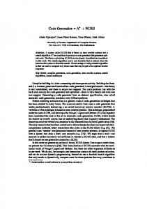
A. Motivating Example We first explain, through the following example, why we need to transform system models for representing the codelevel timed behavior. Consider a system model represented as an event-clock automaton [3] (cf. Definition 2) shown in Figure 1. Each transition in the model is labelled with either an input (a1 ? and a3 ?) or an output (a2 !) event. Each event is associated with a clock, which is automatically reset to zero whenever a transition associated with the corresponding event is taken. For example, the clock xa1 is reset to zero when the transition labelled with the input event a1 ? is taken. Transitions are also annotated with clock guard conditions. For example, the guard condition xa1 ≥ 2 ∧ xa1 ≤ 10 means that the transition can be taken anytime non-deterministically in between 2 and 10 time-unit after the previous transition. It is straightforward to verify that the example model satisfies the following timing constraint (REQ0): “a system shall produce the output a2 ! within 2 and 10 time-unit since the input a1 ? event occurs from the environment”. The timing parameters in the clock guard conditions do not distinguish code-level delays and platform-processing delays. Suppose the platform-processing delay is 2 time units. Then a system implemented using the code generated from the model shown in Figure 1 would not preserve REQ0, because the delay of output a2 ! is now bounded by 4 and 12 time units. This implies that the system model shown in Figure 1 is not an appropriate representation for the code generation. Thus, there is a need for model transformation. In practice, the given platform-processing delays are often in a range (i.e., minimum and maximum bounds) rather than a single constant, which makes the model transformation challenging. Because we need to consider the intermix of min/max platform-processing delays and code-level delays, while the latter may also be affected by the model structure (e.g., loops). Once we know what the ranges of platform delays are, timing guards in the model can be adjusted so that the generated code, running on the platform, would exhibit correct system-level behavior. B. Problem Statement Figure 2 shows an overview of relations between system model, software model, code, platform and implementation. We adopt Parnas’ four-variable model [14] to define the boundaries of an implemented system (shown in the right side of the figure). In the four-variable model, monitored (m) and controlled (c) variables characterize changes of physical environmental quantities; on the other hand, input (i) and output

(o) variables characterize software behavior that interact with the physical environment through input/output devices (i.e., platforms in our work). Based on this variable mapping, we define the boundaries of an implemented system to formalize the problem: io-boundary that separates a platform and the code, and mc-boundary that separates an environment and a platform. Suppose that, for a given platform, the minimum and maximum delays of processing each input/output event is known (cf. Definition 3). The goal is to transform a system model (Ms ) into a software model (Mc ) by compensating the platform-processing delays (P), in order to preserve the timing constraints in the system implementation. We first define three functions: fMs , fSOF , and fIMP , which quantify the min/max delay-bounds of the occurrence of an I/O event succeeding another event in the system model, ioboundary (software model), and mc-boundary, respectively. Formally, we define fMs (i , j ) as the min/max delay-bounds of simple paths (i.e., those without cycles) starting from the transition i and ending with the transition j in the system model Ms . For example, the timing constraint REQ0 can be formally denoted by fMs (1 , 2 )=[2,10], representing that the output transition 2 shall be taken in between 2 and 10 timeunit after taking the input transition 1 of Model 1 shown in Figure 1. Given a simple path p, we can also write fMs (p). We define fSOF and fIMP in a similar fashion as for fMs . In the model transformation from Ms to Mc , we only adjust the timing parameters (i.e., clock guards) and do not change the model structure. Therefore, there are one-to-one mappings between transitions i and j for fMs (i , j ), fSOF (i , j ) and fIMP (i , j ). Definition 1 (Delay-Bound Inclusion Constraint). A system implementation preserves the delay-bound inclusion constraint with respect to the corresponding system model iff: • the minimum delay bound of fIMP for any pair of I/O events at the mc-boundary is no less than that of fMs , • the maximum delay bound of fIMP for any pair of I/O events at the mc-boundary is no greater than that of fMs . Formally, we denote the constraint satisfaction by fIMP (i , j ) ∈ min max (i , j ) and fIMP (i , j ) ≤ fMmax (i , j ) fMs (i , j ) iff fIMP (i , j ) ≥ fMmin s s for any pair of I/O transitions (events) i and j. Example 1. Model 1 shown in Figure 1 has three pairs of I/O transitions, where fMs (1 , 2 )=[2,10], fMs (2 , 3 )=[7,10], fMs (1 , 3 )=[9,20]. The delay-bound inclusion constraint holds for a system implementation with fIMP (1 , 2 )=[4,6], min fIMP (2 , 3 )=[8,9], fIMP (1 , 3 )=[15,19]}, because fIMP ≥ fMmin s max max and fIMP ≤ fMs for all possible pairs of I/O transitions. The key of model transformation from a system model Ms into a software model Mc lies in solving the research problem of finding a suitable function fSOF such that the induced function fIMP (based on the known platform-processing delay P) preserves the delay-bound inclusion constraint with respect to the function fMs (determined by Ms ). We also need to show that any system implementation meeting the delaybound inclusion constraint is guaranteed to satisfy the timing requirements that are verified in the system model Ms . C. Approach Overview Finding a suitable function fSOF is a challenging problem. On the one hand, we need to consider its dependency to the function fIMP and the platform-processing delay P. On the other hand, we need to make sure that the derived function fIMP and the system model function fMs satisfy the delay-bound inclusion constraint. The simple shrinking or expanding timing guards of fMs would not give us a satisfying fSOF , because the

Model Transformation

Software Model ( M c)

System Model ( Ms)

f SOF

2

a1? 1

l 1

L2

u 1

[t , t ]

Platform Processing Delay ( P )

3 c

Environment

Real Environment





f IMP Fig. 3.

We refer to [3] for the formal operational semantics of event-clock automata. An informal semantic description for an example model could be found in Section II-A. In this paper, we consider three different model structure patterns, namely, sequential (e.g., Model 1 shown in Figure 1), alternative (e.g., Model 2 in Figure 3), and cyclic (e.g., Model 3 in Figure 4). A. Computing fMs The computation of the function fMs , which represents the minimum and maximum delay-bounds between two I/O tran-

L3

[t3l , t3u ]

3

1

Definition 2 (Event-Clock Automata). An event-clock automaton is a tuple M= (L, L0 , Lf , Σ, E), where L is a set of locations; L0 ∈ L and Lf ∈ L are an initial and a final location, respectively; Σ = Σin ∪ Σout is an alphabet with a set of input (resp. output) events Σin (resp. Σout ); E = {(L, L0 , a, ϕ)} is a fine set of transitions with each transition connecting a starting location L and an ending location L0 , labelled with an input/output event a ∈ Σ, and associated with a clock constraint ϕ over the clocks CΣ .

[t4l , t4u ]

a4! xa3  4  xa3  8

a3? xa2  7  xa2  10

L1

Fig. 4.

4

Model 2 with variable assignment (Alternative Pattern)

Mapping from system models to implementations

change of timing guards in one transition (e.g., with the intent of decreasing fSOF ) may actually increase fSOF for another transition/path, due to the complex dependency among various I/O transitions and the mixture of minimum/maximum delays. Our approach is to formalize those dependencies in terms of a set of linear constraints to automatically find timing parameter assignments for the function fSOF using the integer linear programming (ILP). First, we propose algorithmic procedures to compute fMs and fIMP . The computation of fMs is based on the timing parameters (i.e., clock guard constants) in the system model Ms , while the computation of fIMP is based on the timing parameters of the software model Mc (represented as variables in fSOF ) and the platform-processing delays P. Then, we formalize the delay-bound inclusion constraint between fMs and fIMP as a set of linear inequality constraints for ILP. A satisfying solution of the ILP problem gives us a set of variable assignments for fSOF , which can be used to parameterize the timing guards of the software model Mc . Finally, we show by Theorem 1 that the system implemented using the code generated from the software model Mc is guaranteed to satisfy the timing requirements (i.e., bounded delays between a pair of I/O events). III. C OMPUTING fMs AND fIMP In this section, we develop algorithmic procedures for computing fMs and fIMP , which are functions that quantify the min/max delay-bound of any pair of I/O transitions and events in the system model and the implementation, respectively. In this paper, we consider system models that are represented as event-clock automata [3].

[t2l , t2u ]

a3? xa1  7  xa1  10

Platform m

Fig. 2.

L1 o

L4

xa1  2  xa1  10

Code

i

f Ms

a2!

Code Generation

2

[t1l , t1u ] a1? xa3  10

L2

[t3l , t3u ]

[t2l , t2u ]

a2! xa1  2  xa1  10

L3

Model 3 with variable assignment (Cyclic Pattern)

sitions in the system model, is non-trivial. Firstly, there can be many different paths in between two transition occurrences. In this case, the path that has the minimum delay can be different from the one that has the maximum delay. Therefore, we need to examine all possible paths between the two transitions in order to compute fMs . Secondly, paths connecting two transitions may include cycles. Since we assume non-negative guard conditions, the minimum delay bound is obtained by considering only a simple path. However, when it comes to the maximum delay bound, it differs depending on how many cycles are taken between the two transitions. For example, in Model 3 (cf. Figure 4), the maximum delay-bound between transitions 1 and 3 increases as more cycles are taken. We first show how to compute fMs for a pair of transitions which are connected by simple paths (i.e., paths that do not contain any repeating locations) only. To this end, we adapt the Floyd-Warshall algorithm. The Floyd-Warshall algorithm computes the minimum and maximum timing intervals between the entering of locations Li and Lj in a model with n locations, denoted by D min (Li , Lj , n) and D max (Li , Lj , n), respectively. We cannot use the Floyd-Warshall algorithm to compute fMs directly, because the function represents the delaybound between two transitions rather than locations. Instead, we define: l fMmin (i , j ) = D min (Lpost , Lpre i j , n) + νj s

fMmax (i , j ) s

=D

max

(Lpost , Lpre i j , n)

+

νju

(1a) (1b)

where Lpost is the ending location of transition i, Lpre i j is the l u starting location of transition j, νj and νj are the lower and upper bounds of clock valuations associated with transition j. For example, Figures 5(a)-(b) show the results of applying the Floyd-Warshall algorithm to Model 3, while Figures 5(c)(d) show the computation results of fMs for Model 3. Note that the values of the main diagonal entries are undefined in Figures 5(c)-(d), because the method described above is only applicable for transitions connected with simple paths. Now, we generalize the computation of fMs for paths with cycles (i.e., non-simple paths). Lemma 1. The min/max delay-bound over a (non-simple) path p in a system model Ms , denoted by fMs (p), is the summation

(a)

(c)

D min L1 L2 L3

L1

L2

L3

0

0

2

9

0

2

7

7

0

f Mmin s

1

2

3

1 2 3

-

2

9

7

-

7

0

2

-

(b)

(d)

D max L1 L1 0 L2 20 L3 10

L2

L3

10

20

0

10

20

0

f Mmax s

1

2

3

1 2 3

-

10

20

20

-

10

10

20

-

delay is given by P={P(a1 )=[1,2],P(a2 )=[3,4],P(a3 )=[2,5]} That is, it takes the platform at least 1 and at most 2 timeunit from the moment it reads the input event a1 (mapped to m variable in Figure 2) from the environment at the mcboundary until the moment the code reads the processed input event (mapped to i variable) at the io-boundary. Similarly, it takes the platform at least 3 and at most 4 time-unit from the moment the code writes the output event a2 (mapped to o variable) at the io-boundary until the moment the platform writes the processed output event (mapped to c variable) to the environment at the mc-boundary. (a) System model behavior

t1?

Fig. 5. The results of applying the Floyd-Warshall algorithm and computing fMs for Model 3

of the min/max delay-bounds of all simple paths that comprise p. Proof: See the Appendix. Note that Lemma 1 is only applicable to event-clock automata where clocks reset on every transition, which is sufficient for this paper. The computation for more general cases (e.g., clocks reset in arbitrary transitions) was studied in [8] using the reachability graph, but that algorithm may not terminate in the presence of cycles. Example 2. Consider a path p in Model 3 that starts with the transition t1 and ends with t3 after repeating two cycles; that is, p=t1 ,t2 ,t3 ,t1 ,t2 ,t3 . The path p consists of the following simple paths: p1 =t1 ,t2 ,t3 ; p2 =t3 ,t1 ,t2 ; and p3 =t2 ,t3 . From Figures 5(c)-(d), we know that fMs (1 , 3 )=[9,20], fMs (3 , 2 )=[2,20], and fMs (2 , 3 )=[7,10]. Based on Lemma 1, we obtain that fMmin (p)=fMmin (1 , 3 )+fMmin (3 , 2 )+fMmin (2 , 3 ) and s s s s max max max max fMs (p)=fMs (1 , 3 )+fMs (3 , 2 )+fMs (2 , 3 ). Thus, we have fMs (p)=[18,50]. B. Computing fIMP In the following, we describe how to compute the function fIMP based on the platform-processing delay P and the codelevel delay fSOF . Definition 3 (Platform-Processing Delay). For any I/O event ak ∈ Σ, the platform-processing delay P(ak ) = [δkmin , δkmax ], where δkmin and δkmax are the minimum and maximum times needed for the platform to process the event ak , respectively. The platform-processing delay characterizes the min/max delays consumed by a given platform (independently of the code-level delays) to process each I/O event. In Figure 2, this delay is considered as the input delay consumed over the information flow from m to i, and the output delay consumed over the information flow from o to c. These delays occurring over the information flows originate from several delay segments that are necessary for the code to interact with its environment via a platform, such as the timing overhead for processing physical input/output signals incurred by device drivers and scheduling delays. More details of such delay segments can be found in our previous work [11] [10], and this paper assumes that the platform-processing delays are bounded as minimum and maximum parameters. Example 3. There are three I/O events {a1 ?, a2 !, a3 ?} in Model 1 shown in Figure 1. Suppose the platform-processing

( xa1  2  xa1  10)  True

t2!

f Ms (1,2)=[2,10]

]

[

time

 M s (1, 2)  8 (b) Implementation behavior (before delay-adjustment) reset( xa1 ) read(a1i )

m 1

a

[

] P(a1 )  [1,2]

(read( xa1 )  2  read( xa1 )  10)  True

fSOF (1,2)=[2,10] f IMP (1,2)=[4,14]

reset( xa2 ) write( a2o )

a2c

]

[ P(a2 )  [1,2]  IMP (1, 2)  10

Fig. 6. The timed behavior comparison between the system model (Ms ) and the implementation (P(a1 )=[1,2] and P(a2 )=[1,2]); the arrows imply the events of the mc-boundary, while the diamond polls imply the events of the io-boundary

Now, we explain the relation between the system implementation delay fIMP , the code-level delay fSOF , and the platformprocessing delay P. For example, Figure 6 illustrates how the system model and the implementation behave differently when processing a pair of the input transition 1 (t1 ) and the output transition 2 (t2 ) of Model 1. In the system model, t2 is taken (lower-direction arrow) in between 2 and 10 time-unit since t1 has been taken (upper-direction arrow); therefore, fMs (1 , 2 )=[2,10]. In the implementation, the delaybound fIMP (1 , 2 ) may differ from fMs (1 , 2 ) if the same timing parameters (Ts ) of Ms is used to implement the code-level delay (fSOF ). Suppose the code is generated using Ts (i.e., 2 and 10), and this code is to be integrated with a platform that has the processing delay: P=[1,2] (assuming that the same min/max bound is applied to all I/O events). Assume that the code interacts with the platform through a set of primitives: read primitive to read the processed input values from the platform or to read current clock values; reset primitive to set the clock values to zero; write primitive to write the output values to the platform. Note that the time instances when these primitives are called by the code are different from the times when the corresponding I/O occurs in the environment, due to the platform delays. This implemented system behaves as follows: when the input (denoted as am 1 ) associated with the transition t1 of Ms is generated from the environment, (1) the platform reads am 1 first at the mc-boundary (red upper arrow); (2) the code reads the processed input (denoted as ai1 ) at the io-boundary sometime after, in between 1 and 2 time-unit (first green diamond poll) due to P(a1 ), and reset the associated clock (xa1 ); (3) the code

produces the output (denoted as ao2 ) at the io-boundary (second diamond poll) in between 2 and 10 time-unit after reading the previous input (ai1 ); (4) the platform processes and writes the output (denoted as ac2 ) to the environment at the mc-boundary (red lower arrow) in between 1 and 2 time-unit due to P(a2 ). Intuitively, fIMP (1 , 2 ) will be larger than fMs (1 , 2 ) (i.e., fIMP 6∈ fMs ) in this case; this deviation occurs since the I/O information flow and P have not been compensated in implementing the code-level delay (fSOF ) (i.e., the code-level delay should have been shrinked for the compensation in this case). (Case 1) Delay-Bound of Input-Output m read(aii ) i

a

[

fSOF (i, j )

a cj

write(a oj )

f IMP (i, j )

]

[

P(ai )

(Case 2) Delay-Bound of Output-Output c write(aio ) i

a

P(ai )

]

P(a j )

fSOF (i, j )

[

time

a cj

write(a oj )

f IMP (i, j ) [

]

]

P(a j )

(Case 3) Delay-Bound of Output-Input

aic

write(aio )

P(ai )

[

]

(Case 4) Delay-Bound of Input-Input m read(aii ) i

a

[

]

f IMP (i, j )

read(a ij )

[

fSOF (i, j )

[

a mj

read(a ij )

]

D ELAY-B OUND A DJUSTMENT USING I NTEGER L INEAR P ROGRAMMING

In this section, we explain how to find the unknown variables (Tc ) that will be used to implement the code-level delay (fSOF ) using the integer linear programming (ILP). A. Intuition of the Delay-Bound Adjustment We formalize the ILP problem to find Tc to generate the code that can be integrated with a platform preserving the delay-bound inclusion constraint with respect to the system model (Ms ). Before explaining the details, the intuition behind this formalization is given. Consider the timed behavior of Ms and the implemented system in Figure 6. In case the code is generated using Ts , two orthogonal aspects result in the deviation of the timed behavior between Ms and the implementation. (1) the deviation of the uncertainty range: the uncertainty range of a pair of I/O transition ti and tj of Ms and the uncertainty range of a pair of the corresponding I/O events of an implemented system is defined as follows: ∆Ms (i, j) = fMmax (i , j ) − fMmin (i , j ) s s ∆IMP (i, j) =

] P(a j )

f IMP (i, j ) P(ai )

a mj

fSOF (i, j )

IV.

P(a j )

Fig. 7. The four cases of the delay bound computation at the implementation level

max fIMP (i , j )

−

(2a)

min fIMP (i , j )

(2b)

This range implies that the time interval where the second transition (tj ) is allowed to occur following the first transition (ti ). However, if the code is generated using the original timing parameter assignment (Ts ), the system model uncertainty (∆Ms ) is directly implemented as a code as well. The issue is that the chosen platform will add another uncertainty that comes from the platform-processing delay (P). For example, in Fig. 6-(b), the uncertainty range of the implementation (∆IMP ) becomes 10 that is larger than the system model uncertainty (∆Ms ) by 2; this additional amount comes from P that results in violation of the delay-bound inclusion constraint. To remedy this, we introduce the Shrinking operation to adjust either upper-bound or lower-bound of the guard condition of the code to compensate P; this will make ∆IMP fit into that of ∆Ms by either increasing the lower-bound or decreasing the upper-bound (i.e., ∆IMP (i, j) ≤ ∆Ms (i, j)). In Figure 8-(c), for example, the uncertainty range of the implementation is reduced by changing the guard condition associated with t2 from [2,10] to [4,10] (i.e., the lower bound of the original guard condition is increased by 2).

In general, fIMP can be larger or smaller than fMs depending on the event type and the amount of the platform-processing delay and the dependency among different transitions; the four possible I/O patterns and their implementation behavior are illustrated in Figure 7. Therefore, it is problematic to generate the code using the same parameters (Ts ) of Ms . Instead, we want to find a new timing parameter assignment (Tc ) that can be used for the code so that the delay-bound inclusion constraint holds. In order to find Tc , we derive the equation of fIMP by separating two parts: we consider the part that constitutes the platform-processing delay (P) as known parameters, while we (c) Impl. behavior after shrinking the guard leave the part that constitutes the code-level delay (fSOF ) as (read( x )  4  read( x )  10)  True unknown variables; now, fIMP for any pair of I/O events can write( a2o ) read(a1i ) be calculated as follows: m a2c a1 fSOF (1,2)=[4,10] Each event (i, j) occurring at the mc-boundary is either input or output, hence there are four combinations for a pair f IMP (1,2)=[6,14] of events that can be calculated as follows: ] [ • Case 1: i is an input event and j is an output event:  IMP (1,2)  8 min max [fSOF (i , j )+(Pmin (aj )+Pmin (ai )), fSOF (i , j )+(Pmax (aj )+Pmax (ai ))] (d) Impl. behavior after shifting the guard • Case 2: i is an output event and j is an output event: min max (read( x )  0  read( x )  6)  True [fSOF (i , j )+(Pmin (aj )−Pmax (ai )), fSOF (i , j )+(Pmax (aj )−Pmin (ai ))] read(a1i ) write( a2o ) • Case 3: i is an output event and j is an input event: m a1 min max a2c fSOF (1,2)=[0,6] [fSOF (i , j )− (Pmax (aj )+Pmax (ai )), fSOF (i , j )−(Pmin (aj )+Pmin (ai ))] • Case 4: i is an input event and j is an input event: f IMP (1,2)=[2,10] min max ] [fSOF (i , j )− (Pmax (aj )−Pmin (ai )), fSOF (i , j )−(Pmin (aj )−Pmax (ai ))] [  IMP (1, 2)  8 These equations are obtained by the straightforward case analysis illustrated in Figure 7. A detailed derivation in given Fig. 8. The illustration of the delay adjustment algorithm in Appendix. a1

a1

a1

a1

time

(2) I/O information flow directions: In spite of the shrinking operation in Figure 8-(c), the resulting fIMP (1 , 2 ) is [6,14] that is not included in fMs (1 , 2 )=[2,10] (i.e. fIMP (1 , 2 ) 6∈ fMs (1 , 2 )). This implies that it is not sufficient to perform the Shrinking operation only in order to obtain Tc . The main reason is that the shrinking operation only makes ∆IMP fit into ∆Ms , but it does not consider the aspects originating from different combinations of I/O information flows. Depending on the types of I/O event pairs, the delay-bound of an implementation is deviated from Ms in four different ways as illustrated in Figure 7. To remedy this, we introduce the Shift operation that moves the relative timing of the second event occurrence back and forth by adjusting both the upper and lower guard condition of the code (c.f., the shrinking operation only adjusts either guard condition). In Figure 8-(d), for example, both the lower and upper guard condition of the code are decreased by 4; the result of this shift operation is that the code should now produce the output in between 0 and 6 time-unit; then the implementation preserves the delay-bound inclusion constraint with respect to Ms (i.e., fIMP (1 , 2 )=[2,10] ∈ fMs (1 , 2 )=[2,10]). Applying the shrinking/shift operations for all possible pairs of I/O transitions is challenging since there are many different aspects intertwined with each other in a complicated pattern, such as the platform-processing delay, the I/O information flows and the dependency among different I/O transitions. Furthermore, these operations may be impossible under certain circumstances (e.g., ∆IMP is too small relative to the amount of the delay that has to be shrinked). We explain how these conditions are formalized in terms of the ILP so that the two operations (i.e., shrinking and shifting) can be automatically performed for all possible I/O transitions to adjust the codelevel delay. B. Formalization of the ILP Problem for Acyclic Models We first explain how the problem is formalized for acyclic models, and then explain how it can be extended to cyclic models. Integer Variable Mapping to the Model: To formalize the ILP problem, we first map integer variables to the system model (Ms ) that express the unknown min/max code-level delay (fSOF ). Here is our mapping: two integer variables, tlk and tuk , are mapped to each transition of Ms ; these variables represent the lower and upper bounds, respectively, of the guard condition associated with the transition. In general, this mapping requires 2n variables if Ms has n transitions. For example, six variables (tl1 ,tu1 ,tl2 ,tu2 ,tl3 ,tu3 ) are used to represent Model 1. This variable mapping enables the min/max codelevel delay (fSOF ) for any pair of I/O transitions to be represented in terms of a linear combination of variables. We will use this representation to define constraints as follows: Defining Linear Constraints: For all pairs of I/O transitions in Ms , we formalize the following constraints using the linear combination of the integer variables: • (Type 1) The minimum delay-bound of the implemented system should be equal or greater than that of Ms (i.e., min fIMP ≥ fMmin ); s • (Type 2) The maximum delay-bound of the implemented max system should be equal or less than that of Ms (i.e., fIMP ≤ fMmax ); s • (Type 3) Each min/max delay-bound of the code should be non-negative; • (Type 4) The minimum delay-bound of the code should be equal or less than the maximum delay bound.

Type 1 and type 2 characterize the delay-bound inclusion constraints of Definition 1; we need the constraints of type 3 and type 4 to obtain only non-negative guard conditions whose minimum delay bound is less than the maximum bound. Example 4 (Linear Constraints for Model 1). Model 1 has three pairs of I/O transitions: (1,2), (2,3), (1,3), and here are the linear constraints: • (C1a) tl2 +Pmin (a2 )+Pmin (a1 )≥2 • (C1b) tu2 +Pmax (a2 )+Pmax (a1 )≤10 • (C2a) tl3 −(Pmax (a3 )+Pmax (a2 ))≥7 • (C2b) tu3 −(Pmin (a3 )+Pmin (a2 ))≤10 • (C3a) tl2 +tl3 −(Pmax (a3 )−Pmin (a1 ))≥9 • (C3b) tu2 +tu3 −(Pmin (a3 )−Pmax (a1 ))≤20 • (C4) tl1 ≥0 ∧ tu1 ≥0 ∧ tl2 ≥0 ∧ tu2 ≥0 ∧ tl3 ≥0 ∧ tu3 ≥0 • (C5) tl1 ≤tu1 ∧ tl2 ≤tu2 ∧ tl3 ≤tu3 Suppose a platform is characterized as P=[1,2], and the code is assumed to be generated from Model 1. In this case, the linear constraints are obtained by plugging in P as follows: (C1a) tl2 ≥0; (C1b) tu2 ≤6; (C2a) tl3 ≥11; (C2b) tu3 ≤12; (C3a) tl2 ≥10; (C3b) tu2 +tu3 ≤19; (C4) tl1 ≥0 ∧ tu1 ≥0 ∧ tl2 ≥0 ∧ tu2 ≥0 ∧ tl3 ≥0 ∧ tu3 ≥0; (C5) tl1 ≤tu1 ∧ tl2 ≤tu2 ∧ tl3 ≤tu3 The constraints (C1a,b), (C2a,b), (C3a,b) are relevant to the pairs of transitions (1,2), (2,3), (1,3), respectively. The constraints (C1a)-(C3a) and (C1b)-(C3b) are the type 1 and type 2 constraints, respectively; the right hand side of these constraints come from the calculated fMs according to Lemma 1, while the left hand side are obtained based on the calculations min max of fIMP in Section III by replacing fSOF (i , j ) and fSOF (i , j ) with the linear combination of (1) the relevant integer variables that express the unknown code-level delay, and (2) the known platform-processing delay. On the other hand, the constraint (C4) and (C5) are the type 3 and type 4 constraints needed independently of the platform-processing delay (P). The linear constraints for Model 2 are also similarly defined, and those constraints and the example are given in Appendix. Defining Objective Functions for Optimization: Our goal is to find the parameter assignments (Tc ) for the unknown variables that satisfy these linear constraints. Note that there can be many possible parameter assignments that satisfy these linear constraints. For example, in Figure 8, the guard condition (lower bound: 0 and upper bound: 6) for the pair of I/O transition allows the code to write an output (ao2 ) in between 0 and 6 time-unit since it has read the input (ai1 ) with the result of fIMP (1 , 2 )=[2,10]. Another possible assignment is (lower bound: 0, upper bound: 1) that results in fIMP (1 , 2 )=[2,5], which still preserves the delay-bound inclusion property with respect to Model 1. To this end, we define optimality in choosing Tc by considering the following aspect: apart from the platform-processing delay (P), the code also requires some computation time for its internal processing; for example, the code computes the output based on the input according to the control law that can be a complex function. Therefore, a better solution is to find Tc that maximizes the room for the internal computation of the code. In the above example, the assignment (lower bound: 0, upper bound: 6) is a better solution than the other assignment (lower bound: 0, upper bound: 1) since the code can have more computation time before producing the second event (i.e, 6 time-unit versus 1 time-unit). Such an optimal assignment can be obtained by defining the objective function that maximizes the uncertainty range of the implementation (∆IMP ) as close as to that of the system model (∆Ms ); this will allow us to find

the largest room for the code computation while preserving the linear constraints. Suppose a system model (Ms ) has n pairs of I/O transitions. Then, we also have n uncertainty ranges for the system model (∆Ms ) and an implemented system (∆IMP ) that corresponds to each pair of I/O transitions. ∆Ms is known since it is calculated from the known Ts , but ∆IMP is unknown since it is calculated from the unknown Tc . Let ∆IMP (k) be the uncertainty range of an implemented system for a particular pair (k) of I/O transitions. Then, the general form of our objective function is as follows: n X maximize ∆IMP (i) (3) i=1

For example, Model 1 has three uncertainty ranges that correspond to the three pairs of I/O transitions. ∆IMP (1, 2) = (tu2 + P max (a2 ) + P max (a1 ))− ∆IMP (2, 3) =

(tu3

− (P

min

(tl2 + P min (a2 ) + P min (a1 )) (a3 ) + P min (a2 )))−

(tl3 − (P max (a3 ) + P max (a2 ))) ∆IMP (1, 3) = (tu2 + tu3 − (P min (a3 ) − P max (a1 )))− (tl2 + tl3 − (P max (a3 ) − P min (a1 ))) The following is the objective function for Model 1: maximize

∆IMP (1, 2) + ∆IMP (2, 3) + ∆IMP (1, 3)

Our solver will find the parameter assignment for the six variables (tl1 ,tu1 ,tl2 ,tu2 ,tl3 ,tu3 ) by maximizing the summation of the uncertainty range of the implementation. Example 5 (Optimal parameter assignment of Model 1). Suppose the code is to be generated from Model 1, and integrated with a platform characterized as P=[1,2]; then the optimal parameter assignment for the code is (tl1 ,tu1 ,tl2 ,tu2 ,tl3 ,tu3 ) = (0, INF, 0, 6, 11, 12), where INF implies the absence of the upper bound. Consider another P=[1,3]; then there is no possible parameter assignment for the code generation. In Example 5, the solver finds no feasible parameter assignment for the code in case the platform with P=[1,3] has to be used. This implies that no code can be generated from Model 1 for this platform by preserving the delaybound inclusion constraint. However, suppose another platform P=[1,2] is chosen whose maximum I/O processing delay is 1 time-unit faster than the previous platform. In this case, the solver can find the optimal parameter assignment that can be used to generate the code running on this platform. The objective function for Model 2 is also similarly defined, and it is given in Appendix with the example of the optimal assignment. We believe that one can define more refined notions of optimality in terms of the internal computation time for the code. One possible notion is to give more internal computation time for a particular I/O transition than the other in case adjusting both ∆IMP equally conforms linear constraints. Accommodating such refined optimality will result in more complex objective functions than Equation 3. Exploring all possible notions of optimality and comparing them to each other is out of the scope of this work.

C. Handling Cyclic Models Note that, if a model contains cycles, there can be an infinite number of paths between a pair of transitions. For example, Model 3 contains a cycle closed by transition 3. Consider a pair of transitions (t1 , t3 ); there are an infinite number of paths, corresponding to the number of times the cycle has been followed. Yet, we want to preserve the delay-bound inclusion property for each of these paths. To this end, we show that it is sufficient to consider only the simple paths through the model to guarantee that the delay-bound inclusion property for arbitrary paths, as follows: Theorem 1. Given a platform processing delay P and a system model Ms , if fIMP (i , j ) ∈ fMs (i , j ) for every pair of transitions ti and tj , then fIMP (p) ∈ fMs (p) for any path p that starts with ti and ends with tj . Proof: See the Appendix. Example 6 (Linear Constraints for Model 3). According to Theorem 1, we only need to consider a finite number of simple paths in Model 3, and the corresponding linear constraints are listed below: • (C1a) tl2 +Pmin (a2 )+Pmin (a1 )≥2 • (C1b) tu2 +Pmax (a2 )+Pmax (a1 )≤10 • (C2a) tl2 +tl3 -(Pmax (a3 )-Pmin (a1 ))≥9 • (C2b) tu2 +tu3 -(Pmin (a3 )-Pmax (a1 ))≤20 • (C3a) tl3 +tl1 -(Pmax (a2 )+Pmax (a1 ))≥7 • (C3b) tu3 +tu1 -(Pmin (a2 )+Pmin (a1 ))≤20 • (C4a) tl3 -(Pmax (a3 )+Pmax (a2 ))≥7 • (C4b) tu3 -(Pmin (a3 )+Pmin (a2 ))≤10 • (C5a) tl3 -(Pmax (a1 )-Pmin (a3 ))≥0 • (C5b) tu3 -(Pmin (a1 )-Pmin (a3 ))≤10 • (C6a) tl1 +tl2 +(Pmin (a3 )+Pmin (a2 ))≥2 • (C6b) tu1 +tu2 +(Pmax (a3 )+Pmax (a2 ))≤20 • (C7) tl1 ≥0 ∧ tu1 ≥0 ∧ tl2 ≥0 ∧ tu2 ≥0 ∧ tl3 ≥0 ∧ tu3 ≥0 • (C8) tl1 ≤tu1 ∧ tl2 ≤tu2 ∧ tl3 ≤tu3 Now, the objective function can be similarly defined as Model 1 and Model 2; the following is the list of uncertainty ranges that correspond to the pairs of I/O transitions in Model 3: ∆IMP (1, 2) = (tu2 + P max (a2 ) + P max (a1 ))− (tl2 + P min (a2 ) + P min (a1 )) ∆IMP (1, 3) = (tu2 + tu3 − (P min (a3 ) − P max (a1 )))− ∆IMP (2, 1) =

(tu3

+

tu1

(tl2 + tl3 − (P max (a3 ) − P min (a1 ))) − (P min (a2 ) + P min (a1 )))−

(tl3 + tl1 − (P max (a2 ) + P max (a1 ))) ∆IMP (2, 3) = (tu3 − (P min (a3 ) + P min (a2 )))− ∆IMP (3, 1) =

(tu3

− (P

∆IMP (3, 2) =

(tu1

tu2

+

min

(tl3 − (P max (a3 ) + P max (a2 ))) (a1 ) − P max (a3 )))−

(tl3 − (P max (a1 ) − P min (a3 ))) + (P max (a3 ) + P max (a2 )))− (tl1 + tl2 + (P min (a3 ) + P min (a2 )))

The following is the objective function for Model 3: maximize

∆IMP (1, 2) + ∆IMP (1, 3) + ∆IMP (2, 1)+ ∆IMP (2, 3) + ∆IMP (3, 1) + ∆IMP (3, 2)

Example 7 (Optimal parameter assignment of Model 3). Suppose the code is to be generated from Model 3, and integrated with a platform characterized as P=[0,1]; then the optimal parameter assignment for the code is (tl1 ,tu1 ,tl2 ,tu2 ,tl3 ,tu3 ) = (0, 10, 2, 8, 9, 9). Consider another P=[1,2]; then there is no possible parameter assignment for the code generation. V. C ASE S TUDY: I NFUSION P UMP S YSTEMS An infusion pump is a safety-critical medical device that injects drugs to a patient’s body in a controlled manner for medical purposes, such as diabetes treatments or anesthesia. Its hardware platform is equipped with sensors (e.g., a bolus request button, empty reservoir switch) and actuators (e.g., a pump motor, alarm buzzer) to interact with its physical environment (e.g., patient). For example, a patient presses a bolus request button to request an additional amount of drugs; a pump rotates a pump-motor that generates physical forces to move a loaded syringe so that drug can flow from the syringe to the patient. In addition, the pump should detect various alarming conditions using sensor input (e.g., empty/low reservoir condition) to generate alarm signals to caregivers in a timely manner. In order to show the applicability of the proposed approach, we generate the code for the Baxter II Syringe PCA infusion pump platform used for the GPCA reference implementation project [9], and validated several delay-bound inclusion constraints (the equipment setup is shown in Appendix). Here are the details of the case study: (1) Modeling and verification for the infusion pump systems: Model 4 in Figure 9 is the system model (Ms ) used for this case study, and its informal semantics and the implication in the actual PCA pump implementation are as follows: in the initial location (L1 ), the pump waits for the patient’s bolus request (in the implementation, the input mBolusReq is generated by pressing a button). However, the pump shall not accept a bolus request occurring earlier than 5000 ms 1 since the previous infusion has been either normally finished by providing the expected amount of drugs or abnormally finished due to the alarming condition (i.e, those premature bolus requests should be ignored). Otherwise, the pump shall process any valid bolus request by taking the transition from L1 to L2 . In L2 , the pump shall initiate the bolus infusion in between 150 ms and 470 ms by taking the transition from L2 to L3 (in the implementation, the output cStartInf usion is produced by rotating the pump motor at a calculated speed). Any bolus infusion will finish in between 300 ms and 750 ms by taking the transition from L3 to L1 (in the implementation, the output cStopInf usion is produced by stopping the pump motor rotation), unless it encounters the empty syringe condition. During the infusion, if the empty syringe is detected (in the implementation, the input mEmptySyringe is detected from the switch sensor that is pressed when the syringe hits the bottom), the pump takes a transition from L3 to L4 to prepare alarms. In L4 , the pump raises an alarm in between 200 ms and 500 ms by taking the transition from L4 to L1 (in the implementation, the output cAlarm is produced by providing signals to a buzzer and alarm LEDs). Here are three timing constraints considered in this case study: • (REQ1) When a patient requests a bolus, the bolus infusion should start in between 150 ms and 470 ms; 1 We assume 1 time unit in the model is mapped to 1 ms in the implementation

• •

(REQ2) The bolus infusion should be active at least 300 ms, and at most 750 ms; (REQ3) When a patient requests a bolus, the bolus infusion should finish in between 450 ms and 1220 ms in the absense of the empty reservoir alarm. 3 cStopInfusion! xcStartInfusion  300  xcStartInfusion  750

1

[t1l , t1u ]

mBolusReq? xcStopInfusion  5000 

L1

2 L2

xcAlarm  5000

5

[t2l , t2u ]

cStartInfusion! xmBolusReq  150 

L3

xmBolusReq  470

[t5l , t5u ]

4

cAlarm! xmEmptySyringe  200 

[t3l , t3u ]

L4

[t4l , t4u ]

mEmptySyringe? xcStartInfusion  1500

xmEmptySyringe  500

Fig. 9.

Model 4 with variable assignment (Simplified GPCA model)

(2) Obtaining the platform-processing delay (P): We measured the platform-processing delay (P) of each input and output of the Baxter PCA pump according to the measurement method introduced in [11], and here is the brief explanation: To measure the input processing delay, we obtained the timestamp (tm ) when the input is generated from the environment (mc-boundary), and obtained another timestamp (ti ) when the code reads the processed input (io-boundary); the input processing delay is calculated by subtracting tm from ti . To measure the output processing delay, we obtained the timestamp (to ) when the output is generated from the code (io-boundary), and another timestamp (tc ) when the platform actually writes the processed output to the environment (mcboundary); the output processing delay is calculated by subtracting to from tc . We obtained each timestamp using the oscilloscope that captures the signal changes of the sensors and actuators of the PCA pump (the example of this oscilloscope measurement is given in Appendix). The measurement has been performed 20 times to measure each I/O delay (two inputs and three outputs), and the min/max bound and the average of the measured platform processing delay are summarized in Table. I. I/O Event

Type

 (ms) Pmax

Avg. (ms)

mBolusReq? cStartInfusion! cStopInfusion! mEmptySyringe? cAlarm!

Input

50

151

105.27

Output

100

303

225.97

Output

98

302

213.64

Input

104

200

142.8

Output

298

303

300.05

TABLE I.

 (ms) Pmin

T HE MEASURED PLATFORM PROCESSING DELAY OF THE BAXTER II SYRINGE PUMP PLATFORM

From this measurement, we characterize the platformprocessing delay of the Baxter PCA pump platform as P={P(mBolusReq)=[50,151],P(cStartInfusion)=[100,303], P(cStopInfusion)=[98,302],P(mEmptySyringe)=[104,200], P(cAlarm)=[298,303]}. (3) Formalizing the ILP problem: According to the procedure explained in Section IV, we formalized the ILP problem to find the optimal parameter assignment to generate the code. Firstly, two integer variables are mapped to each I/O transition of the

model, which are unknown variables that need to be solved to implement the code-level delay; a total of 10 integer variables are mapped to the model (tl1 ,tu1 ,tl2 ,tu2 ,tl3 ,tu3 ,tl4 ,tu4 ,tl5 ,tu5 ). Secondly, fMs has been calculated for the simple paths between all pairs of I/O transitions; a total of 20 pairs of fMs are calculated. Thirdly, based on the calculated fMs , 42 linear constraints have been formalized that need to be satisfied for delay-bound inclusion constraint. Finally, the objective function is defined with the given P, and the solver finds the optimal parameter assignment as summarized in Table II. This parameter assignment is used to implement the guard conditions in generating the code that will be executing on the given platform. t1l

t1u

t2l

t2u

t3l

t3u

t4l

t4u

t5l

t5u

T Ms

5000

INF

150

470

300

750

0

1500

200

500

T Mc

5454

INF

0

16

505

548

503

1704

0

202

TABLE II.

T HE PARAMETER ASSIGNMENT (Ts ) OF Ms AND THE PARAMETER ASSIGNMENT (Tc ) OF Mc

(4) Validating the optimal solution: The goal of the validation is to compare how well the two different codes generated from the system model (Ms ) and the software model (Mc ) preserve the delay-bound inclusion constraint. We generated the two different codes from each model using the TIMES tool [4]. In order to obtain the implemented system, the generated codes are interfaced with the same platform-specific I/O processing routines whose min/max processing delay-bound is measured as shown in Table I. In order to validate the delay-bound inclusion constraint, we measured the delay between a pair of I/O events associated with each timing constraint at the mc-boundary. For example, in order to validate REQ1, we obtained the timestamp (tmBolusReq ) for the signal change occurring at the bolus request button (its signal changes from 5 volts to 0 volts if the button is pressed by the patient); and we obtained another timestamp (tcStartInf usion ) for the signal change occurring at the pump motor (its signal changes from 0 volts to 5 volts if the motor starts rotating); the delay between the two signal changes are measured by subtracting tmBolusReq from tcStartInf usion . For each code, the delay measurement has been performed 20 times for each timing constraint; the trends of the delaybound for each constraint throughout the testing are shown in Figure 10 11 12; their min/max/average delays are summarized in the two separate fIMP columns of Table III; at the same time, fMs is also shown in Table III as well for comparison. f IMP (T M s , P  )

f Ms

REQ

f IMP (T M c , P  )

Min (ms)

Max(ms)

Min(ms)

Max(ms)

Avg.(ms)

Min(ms)

Max(ms)

Avg.(ms)

REQ1

150

470

603

843

695.8

155

459

283.4

REQ2

300

750

603

907

845

595

619

606.6

REQ3

450

1220

1400

1710

1537

747

1070

887.55

TABLE III. T HE VALIDATION RESULT OF THE DELAY- BOUND INCLUSION CONSTRAINT OF THE GPCA REFERENCE IMPLEMENTATION

Analysis: Meeting the delay-bound inclusion constraint means that all the measured implementation delays of each timing constraint should be within the time interval allowed by the min max system model (Ms ) (i.e., fIMP ≥ fMmin and fIMP ≤ fMmax ). If at s s least one delay measurement is out of the interval allowed by Ms , the implementation does not conform to the delay-bound inclusion constraint. Figure 10, 11, 12 show the validation result of REQ1, REQ2, REQ3, respectively. The purple line and and green line represent fMmin and fMmax , respectively. Hence, the implementation s s

(ms) 900

Delay Bound of REQ1

800 700 600 500

Max bound

400 300 200 Min bound

100 0

1

2

3

4

5

Original

Fig. 10.

6

7

8

Adjusted

9 10 11 12 13 14 15 16 17 18 19 20 (test num) Min Bound (Model)

Max Bound (Model)

Validation Result for REQ1

(ms) 1000

Delay Bound of REQ2

900 800

Max bound

700 600 500

400 300

Min bound

200 100

0 1

2

3 Original

Fig. 11.

4

5

6

7

Adjusted

8

9 10 11 12 13 14 15 16 17 18 19 20 (test num) Min Bound (Model)

Max Bound (Model)

Validation Result for REQ2

delay (fIMP ) is expected to stay within these min/max bounds. The blue line represents the actual delay of the implemented system that executes the code generated from the system model (Ms ) without any delay adjustment; on the other hand, the red line represents the actual delay of the implemented system that executes the code generated from the software model (Mc ) that has been constructed according to the proposed approach. According to our testing results, all measured implementation delays of the system running the code generated from Mc are within the delay-bound allowed by Ms for the three timing constraints (i.e., the delay-bound inclusion constraint holds under this testing set). On the other hand, most measured implementation delays of the system running the code generated from Ms are out of the interval allowed by Ms for all three timing constraints (i.e., the delay-bound inclusion constraint does not hold under this testing set). This result shows that a system model (Ms ) is not an appropriate model to generate the code for the timing constraint conformance; instead, a software model (Mc ) has to be used to generate the code toward the timing constraint conformance. VI.

R ELATED W ORK

There have been a number of works to incorporate the platform processing delay in high level models in several different ways. [16] proposed a parametric semantics that allows the reaction time of a platform to be modeled, and an analytic method to check if a platform has sufficient processing power for property preservation. On the other hand, [2] proposed a way to explicitly model software and platforms together to abstract the timed behavior of an implementation. Their approach includes platform modeling such as, digital clock, program execution and I/O interfaces, so that the

(ms) 1800

Delay Bound of REQ3

1600 1400 Max bound

1200 1000

800 600 400

Min bound

200

0 1

2

3 Original

Fig. 12.

4

5

6

7

Adjusted

8

9 10 11 12 13 14 (test num) Min Bound (Model)

15

16

17

18

19

20

Max Bound (Model)

Validation Result for REQ3

collection of these models can be checked for the property preservation of an implementation. [1] [15] also studied how platform-specific timing delays can be incorporated with the platform-independent model. Their approach is to transform the platform-independent model into a physical model by decomposing each action transition in two separate transitions to express the platform-overhead required for processing events of the platform-independent model. Even though these platform models proposed in each work [16] [2] [1] [15] are useful in analyzing the property preservation of an implementation, these works lack of consideration as to how software part can be generated and integrated with a platform in a way the implementation still holds the property. Furthermore, their platform models are rather too abstract by ignoring some aspects that result in the timed behavior deviation between a model and an implementation. For example, these works lack of consideration as to how I/O dependency and information flow that affect to the timed behavior of an implementation w.r.t. its model. In comparison to the above works and our work that considered the timed automata semantics in characterizing timing aspects of platforms, there are other works that express the timing aspects in different ways. AADL [6] introduced several components that can express platform’s timing aspects such as threads, port connections, and bus components; TrueTime [7] introduced kernel and network blocks that can be connected to the ordinary Simulink blocks so that the temporal behavior of a system that executes control algorithms on a particular platform can be simulated. Even though these modeling strategies do not discuss about the code generation, we believe that the way these works abstract the timing aspects of platforms can complement our work in refining the definition of the platform processing delays. Regarding to the delay-bound computation, [5] defined three quantitative refinement metrics -(a) maximum time difference, (b) eventual maximum time difference, (c) average time difference.- that quantify the timing mismatches between a model and its implemented systems. Even though this work does not consider how to obtain code from the timed models, we believe that these are more refined metrics to reason about the relationship between a model and its implementations compared to our delay-bound inclusion constraint. We leave applying these metrics to extend our code generation framework as a future work. VII. C ONCLUSION AND F UTURE W ORK We proposed a way to transform a system model (Ms ) into a software model (Mc ) in order to compensate the platformprocessing delays (P) for code generation purpose. Our model

transformation is performed by formalizing it using integer linear programming in order to preserve the delay-bound inclusion constraint at the implementation level. This approach provides two types of automation in the code generation process: (1) given a platform, it automatically checks whether there exists a code generation strategy that preserves the delaybound inclusion constraint; (2) (if it is feasible), the software model (Mc ) is automatically obtained from the system model (Ms ), which guarantees to generate optimal code that can utilize the maximum computation time in between processing any pairs of I/O events. Our case study using the infusion pump system shows the code generated from Mc better preserves the delay-bound inclusion constraints compared to the code generated from Ms . As a future work, we plan to study a broader scope of modeling patterns that can be applicable for computation of fMs and fIMP . We also plan to extend a notion of platforms to the distributed setting. That is, a system model abstracts timed behavior of distributed systems; and several different code should be generated running on each platform that are connected through network. This requires more refined definition of the platform-processing delays (e.g., incorporating network delays) and a new model transformation strategy for code generation. R EFERENCES [1] [2] [3]

[4]

[5]

[6]

[7]

[8]

[9]

[10]

[11]

[12]

[13] [14] [15]

[16]

Tesnim Abdellatif, Jacques Combaz, and Joseph Sifakis. Model-based implementation of real-time applications. In EMSOFT. ACM, 2010. K. Altisen and S. Tripakis. Implementation of timed automata : an issue of semantics or modeling. FORMATS, 2005. Rajeev Alur, Limor Fix, and Thomas A. Henzinger. Event-clock automata: a determinizable class of timed automata. Theoretical Computer Science, 211(12):253 – 273, 1999. T. Amnell, E. Fersman, L. Mokrushin, P. Pettersson, and W. Yi. TIMES: a tool for schedulability analysis and code generation of real-time systems. In FORMATS, 2003. Krishnendu Chatterjee and Vinayak S. Prabhu. Quantitative timed simulation functions and refinement metrics for real-time systems. HSCC ’13, pages 273–282, New York, NY, USA, 2013. ACM. Peter H Feiler, David P Gluch, and John J Hudak. The architecture analysis & design language (aadl): An introduction. Technical report, DTIC Document, 2006. Dan Henriksson, Anton Cervin, and Karl erik rzn. Truetime: Real-time control system simulation with matlab/simulink. In Proc. of the Nordic MATLAB Conference, 2003. Inhye Kang and Insup Lee. An efficient state space generation for analysis of real-time systems. SIGSOFT Softw. Eng. Notes, 21(3):4–13, May 1996. Baek Gyu Kim, A. Ayoub, O. Sokolsky, Insup Lee, P. Jones, Yi Zhang, and R. Jetley. Safety-assured development of the gpca infusion pump software. In EMSOFT ’11, pages 155–164, Oct 2011. BaekGyu Kim, Lu Feng, Linh T. X. Phan, Oleg Sokolsky, and Insup Lee. Platform-specific timing verification framework in model-based implementation. DATE ’15, pages 235–240, 2015. BaekGyu Kim, Hyeon I Hwang, Taejoon Park, Sang H. Son, and Insup Lee. A layered approach for testing timing in the model-based implementation. In DATE ’14, pages 1–4, March 2014. BaekGyu Kim, Linh T. X. Phan, Oleg Sokolsky, and Insup Lee. Platform-dependent code generation for embedded real-time software. In CASES ’13. IEEE Press, 2013. MathWorks. Simulink coder - generate c and c++ code from simulink and stateflow models. David Lorge Parnas and Jan Madey. Functional documents for computer systems. Science of Computer Programming, 25:41–61, 1995. Ahlem Triki, Jacques Combaz, Saddek Bensalem, and Joseph Sifakis. Model-based implementation of parallel real-time systems. In FASE ’13. 2013. Martin Wulf, Laurent Doyen, and Jean-Franois Raskin. Almost asap semantics: From timed models to timed implementations. In HSCC. 2004.

Proof: Suppose p consists of a series of transitions ti . . . tj , where ti is the starting transition of p, and tj is the ending transition of p. Let tp1 . . . tpk be the ending (and starting) transitions in between ti and tj that comprises all Notations Definitions simple paths ∈ p; that is, p = ti . . . tp1 . . . tp2 . . . tpk . . . tj with a set The system model Ms of simple paths ti . . . tp1 , and tp1 . . . tp2 ,. . . , and tpk−1 . . . tpk , and The software model Mc tpk . . . tj . In an event-clock automaton, the min/max interval The timing parameter assignments to the system model and the software model Ts , Tc of a particular simple path can be calculated independently The lower/upper bound of clock values associated with a transition k of the software model tkl , tku The lower/upper bound of clock values associated with a transition k in the system model of the min/max interval of its adjacent simple paths (i.e., the  kl , ku The min/max platform processing delay of the event a ; P( ak ) min/max interval of a prior simple path immediately followed By adding min and max superscript, each indicates minimum delay bound and maximum delay bound separately. [P (a ), P (a )] by this simple path, and the post simple path immediately The min/max delay bound of a transition j succeeding a transition i in the system model; f M (i , j ) By adding min and max superscript, each indicates minimum delay bound and maximum delay following this simple path) using an event-recording clock min max [ f M (i, j ), f M (i, j )] bound separately that is reset to zero upon taking a starting transition of a The min/max delay bound of a path p in the system model; f M ( p) By adding min and max superscript, each indicates minimum delay bound and maximum delay [ f ( p), f ( p)] simple path. Therefore, the minimum interval of fMs (p) is bound separately The min/max delay bound of an event j (corresponding to transition j in the system model) f IMP (i, j ) calculated as follows: fMmin (p) = fMmin (ti , t1p ) + fMmin (t1p , t2p ) + succeeding an event i (corresponding to transition i in the system model) at the mc-boundary; By s s s min max p p p adding min and max superscript, each indicates minimum delay bound and maximum delay bound min min [ f IMP (i, j ), f IMP (i, j )] separately . . . + fMs (tk −1 , tk ) + fMs (tk , tj ); and the maximum interval The min/max delay bound of a final event (corresponding to the final transition of p in the system f IMP ( p ) of fMs (p) is also similarly calculated. model) succeeding a start event (corresponding to the start transition of p in the system model) at min max mc-boundary; By adding min and max superscript, each indicates minimum delay bound and [ f IMP ( p), f IMP ( p)] the Theorem 1 Given a platform processing delay P and a maximum delay bound separately The min/max delay bound of an event j (corresponding to transition j in the system model) system model Ms , if fIMP (i , j ) ∈ fMs (i , j ) for all possible pair fSOF (i, j ) succeeding an event i (corresponding to transition i in the system model) at the io-boundary; adding min and max superscript, each indicates minimum delay bound and maximum delay min max of transitions ti and tj , then fIMP (p) ∈ fMs (p) for all paths p [ fSOF (i, j ), fSOF (i, j )] By bound separately The system model-level input/output event (identifier: k) that starts with ti and ends with tj . ak?, ak! The implementation-level input event: the input (m) generated from the environment at the mcm i Proof: (Proof by contradiction) Suppose ∃ p such that ak , ak boundary; the input (i) processed by the platform at the io-boundary (identifier: k) o c f (p) 6∈ fMs (p), where p = ti . . . tp1 . . . tp2 . . . tpk . . . tj with a The implementation-level output event: the output (o) generated by the code at the io-boundary; IMP ak , ak the output (c) generated by the platform at the mc-boundary (identifier: k) set of simple paths ti . . . tp1 , and tp1 . . . tp2 , . . . , and tpk−1 . . . tpk , xa The event clock associated with the event a p and tk . . . tj . By Lemma 1, fMs (p) is calculated as follows: The uncertainty range of the event j occurrence following the event i occurrence in the system  M (i , j ) model The uncertainty range of the event j occurrence following the event i occurrence in the implemented fMmin (p)=fMmin (ti , t1p )+fMmin (t1p , t2p )+. . . +fMmin (tkp−1 , tkp )+fMmin (tkp , tj )  IMP (i, j ) s s s s s system p p max max max p p max p max p fMs (p)=fMs (ti , t1 )+fMs (t1 , t2 )+. . . +fMs (tk −1 , tk )+fMs (tk , tj ) TABLE IV. N OTATIONS USED IN THE PAPER Since fIMP (p) 6∈ fMs (p), either of the following cases must B. Computation of fIMP (i , j ) be satisfied: Computation of fIMP (i , j ) follows the case analysis for the min (Case 1) fIMP (p) < fMmin (p) s four cases illustrated in Figure 7. We only show Case 1 since max (Case 2) fIMP (p) > fMmax (p) s the rest of the equations are similarly derived. Suppose (Case 1) holds; then, (Case 1: input ti and output tj ) Refer to the information min min p p min p min p fIMP (ti , t1p )+fIMP (t1 , t2 )+. . . +fIMP (tk −1 , tkp )+fIMP (tk , tj ) < flow of Case 1 in Figure 7. Suppose the code reads the input p p min min p p min p min p f (t , t )+f (t , t )+. . . +f (t , t )+f i 1 i at τi and the code writes the output j at τj at the io1 2 Ms Ms Ms Ms (tk , tj ). k −1 k However, this is not possible due to the assumption that boundary. The possible range of the input occurrence at the min fIMP (ti , tj ) ≥ fMmin (ti , tj ) for ∀ ti , tj . mc-boundary is [τi −Pmax (ai ), τi −Pmin (ai )] because the input s Suppose (Case 2) holds; then, at the mc-boundary has to occur before reading the input at max max p p max p max p fIMP (ti , t1p )+fIMP (t1 , t2 )+. . . +fIMP (tk −1 , tkp )+fIMP (tk , tj ) > the io-boundary. The possible range of the output occurrence p p max max p p max p min max fMs (ti , t1 )+fMs (t1 , t2 )+. . . +fMs (tk −1 , tk )+fMmax (tkp , tj ). at the mc-boundary is [τj +P (aj ), τj +P (aj )] because s However, this is not possible due to the assumption that the output at the mc-boundary has to occur after writing the max fIMP (ti , tj ) ≤ fMmax (ti , tj ) for ∀ ti , tj . output at the io-boundary. Then, the minimum interval of these s min min This constradicts the fact that either (Case 1) or (Case 2) two events is (τj +P (aj ))−(τi −P (ai )); the maximum must be satisfied. interval of these two events is (τj +Pmax (aj ))−(τi −Pmax (ai )). By rewriting, the min/max interval of the two event D. ILP Formalization of Model 2 is [τj −τi +Pmin (aj )+Pmin (ai ), τj −τi +Pmax (aj )+Pmax (ai )]. Example 8 (Linear Constraints for Model 2). Model 2 has Note that, the term τj −τi is the code-level delay-bound that four pairs of I/O transitions: (1,2), (1,3), (1,4), (3,4), and here is unknown; the minimum interval of the two events can be are the linear constraints: obtained by having the minimum interval of the code-level • (C1a) tl2 +Pmin (a2 )+Pmin (a1 )≥2 delay; hence, the term τj −τi of the minimum interval is • (C1b) tu2 +Pmax (a2 )+Pmax (a1 )≤10 min rewritten as fSOF (i , j ) that indicates the unknown minimum • (C2a) tl3 −(Pmax (a3 )−Pmin (a1 ))≥7 interval of the code-level delay. The maximum interval of the • (C2b) tu3 −(Pmin (a3 )−Pmax (a1 ))≤10 two events can be obtained by having the maximum interval of • (C3a) tl3 +tl4 +(Pmin (a4 )+Pmin (a1 ))≥11 the code-level delay; hence, the term τj −τi of the maximum • (C3b) tu3 +tu4 +(Pmax (a4 )+Pmax (a1 ))≤18 max interval is rewritten as fSOF (i , j ) that indicates the unknown • (C4a) tl4 +(Pmin (a4 )+Pmin (a3 ))≥4 maximum interval of the code-level delay. As a result, we • (C4b) tu4 +(Pmax (a4 )+Pmax (a3 ))≤8 obtain the final equation of fIMP (i , j ) for Case 1 as follows: • (C5) tl1 ≥0 ∧ tu1 ≥0 ∧ tl2 ≥0 ∧ tu2 ≥0 ∧ tl3 ≥0 ∧ tu3 ≥0∧ min max [fSOF (i , j )+( Pmin (aj )+Pmin (ai )), fSOF (i , j )+(Pmax (aj )+Pmax (ai ))] tl4 ≥0∧ tu4 ≥0 C. Proofs of Lemma and Theorem • (C6) tl1 ≤tu1 ∧ tl2 ≤tu2 ∧ tl3 ≤tu3 ∧ tl4 ≤tu4 Lemma 1 The min/max delay-bound over an (non-simple) Suppose a platform is given characterized as P=[2,4]; and path p in a system model Ms , denoted by fMs (p), is the the code is assumed to be generated from Model 2. The summation of the min/max delay-bounds of all simple paths corresponding linear constraints are as follows: (C1a) tl2 ≥−2; that comprise p. (C1b) tu2 ≤2; (C2a) tl3 ≥9; (C2b) tu3 ≤8; (C3a) tl3 ≥7; (C3b) A PPENDIX A. Notations Table IV list the notations used in the paper.

k

min

max

k

k

s

s

s

s

min Ms ,

max Ms

k

s

k

tu3 +tu4 ≤10; (C4a) tl4 ≥0; (C4b) tu4 ≤0; (C5) tl1 ≥0 ∧ tu1 ≥0 ∧ tl2 ≥0 ∧ tu2 ≥0 ∧ tl3 ≥0 ∧ tu3 ≥0∧ tl4 ≥0∧ tu4 ≥0; (C6) tl1 ≤tu1 ∧ tl2 ≤tu2 ∧ tl3 ≤tu3 ∧ tl4 ≤tu4 Model 2 has four uncertainty ranges that correspond to the four pairs of I/O transitions. ∆IMP (1, 2) = (tu2 + P max (a2 ) + P max (a1 ))− (tl2 + P min (a2 ) + P min (a1 )) ∆IMP (1, 3) = (tu3 − (P min (a3 ) − P max (a1 )))− (tl3 − (P max (a3 ) − P min (a1 ))) ∆IMP (1, 4) = (tu3 + tu4 + (P max (a4 ) + P max (a1 )))− ∆IMP (3, 4) =

(tu4

+ (P

max

(tl3 + tl4 + (P min (a4 ) + P min (a1 ))) (a4 ) + P max (a3 )))− (tl4 + (P min (a4 ) + P min (a3 )))

The following is the objective function for Model 2: maximize ∆IMP (1, 2) + ∆IMP (1, 3) + ∆IMP (1, 4) + ∆IMP (3, 4) This objective function is obtained in a similar way with Model 1 case. Our solver will find the parameter assignment for the eight variables (tl1 ,tu1 ,tl2 ,tu2 ,tl3 ,tu3 ,tl4 ,tu4 ). Example 9 (Optimal parameter assignment of Model 2). Suppose the code is to be generated from Model 2, and integrated with a platform characterized as P=[2,4]; then there is no possible parameter assignment for the code. Suppose the code is to be generated from the same model, and integrated with another platform characterized as P=[2,3]; then the optimal parameter assignment for the code is (tl1 ,tu1 ,tl2 ,tu2 ,tl3 ,tu3 ,tl4 ,tu4 ) = (0, INF, 0, 4, 8, 9, 0, 2). In Example 9, the solver finds no fesible parameter assignment for the code in case the platform with P=[2,4] has to be used. This implies no code can be generated from Model 2 for this platform by preserving the delay-bound inclusion constraint. However, suppose another platform P=[2,3] is chosen whose maximum I/O processing delay is 1 time-unit faster than the previous platform. In this case, the solver can find the optimal paramter assignment that can be used to generate the code running on this platform. E. ILP Formalization of Model 4 Model 4 has total 42 linear constraints as follows: • (C1a) tl2 +Pmin (a2 )+Pmin (a1 )≥ 150 • (C1b) tu2 +Pmax (a2 )+Pmax (a1 )≤ 600 • (C2a) tl2 +tl3 +Pmin (a3 )+Pmin (a1 )≥ 900 • (C2b) tu2 +tu3 +Pmax (a3 )+Pmax (a1 )≤ 2100 • (C3a) tl2 +tl4 −(Pmax (a4 )−Pmin (a1 ))≥ 150 • (C3b) tu2 +tu4 −(Pmin (a4 )−Pmax (a1 ))≤ 2100 • (C4a) tl2 +tl4 +tl5 +Pmin (a5 )+Pmin (a1 )≥ 350 • (C4b) tu2 +tu4 +tu5 +Pmax (a5 )+Pmax (a1 )≤ 2600 • (C5a) min[tl3 +tl1 −(Pmax (a1 )+Pmax (a2 )), tl4 +tl5 +tl1 −(Pmax (a1 )+Pmax (a2 ))] ≥ 5200 • (C5b) max[tu3 +tu1 −(Pmin (a1 )+Pmin (a2 )), tu4 +tu5 +tu1 −(Pmin (a1 )+Pmin (a2 ))]≤ INF • (C6a) tl3 +Pmin (a3 )−Pmax (a2 )≥ 750 • (C6b) tu3 +Pmax (a3 )−Pmin (a2 )≤ 1500 • (C7a) tl4 −(Pmax (a4 )+Pmax (a2 ))≥ 0 • (C7b) tu4 −(Pmin (a4 )+Pmin (a2 ))≤ 1500 • (C8a) tl4 +tl5 +(Pmin (a5 )−Pmax (a2 ))≥ 200 • (C8b) tu4 +tu5 +(Pmax (a5 )−Pmin (a2 ))≤ 2000 • (C9a) tl1 −(Pmax (a3 )+Pmax (a1 ))≥ 5000 • (C9b) tu1 −(Pmin (a3 )+Pmin (a1 ))≤ INF • (C10a) tl1 +tl2 +(Pmin (a3 )−Pmax (a2 ))≥ 5150

(C10b) tu1 +tu2 +(Pmax (a3 )−Pmin (a2 ))≤ INF (C11a) tl1 +tl2 +tl4 −(Pmax (a4 )+Pmax (a3 ))≥ 5150 (C11b) tu1 +tu2 +tu4 −(Pmin (a4 )+Pmin (a3 ))≤ INF (C12a) tl1 +tl2 +tl4 +tl5 +(Pmin (a5 )−Pmax (a3 ))≥ 5350 (C12b) tu1 +tu2 +tu4 +tu5 +(Pmax (a5 )−Pmin (a3 ))≤ INF (C13a) tl5 +tl1 −(Pmax (a1 )−Pmin (a4 ))≥ 5200 (C13b) tu5 +tu1 −(Pmin (a1 )−Pmax (a4 ))≤ INF (C14a) tl5 +tl1 +tl2 +Pmin (a2 )+Pmin (a4 )≥ 5350 (C14b) tu5 +tu1 +tu2 +Pmax (a2 )+Pmax (a4 )≤ INF (C15a) tl5 +tl1 +tl2 +tl3 +Pmin (a3 )+Pmin (a4 )≥ 6100 (C15b) tu5 +tu1 +tu2 +tu3 +Pmax (a3 )+Pmax (a4 )≤ INF (C16a) tl5 +Pmin (a5 )+Pmin (a4 )≥ 200 (C16b) tu5 +Pmax (a5 )+Pmax (a4 )≤ 500 (C17a) tl1 −(Pmax (a5 )+Pmax (a1 ))≥ 5000 (C17b) tu1 −(Pmin (a5 )+Pmin (a1 ))≤ INF (C18a) tl1 +tl2 +(Pmin (a2 )−Pmax (a5 ))≥ 5150 (C18b) tu1 +tu2 +(Pmax (a2 )−Pmin (a5 ))≤ INF 5 (C19a) tl1 +tl2 +tl3 +(Pmin (a3 )−Pmax )≥ 5900 u u u max (C19b) t1 +t2 +t3 +(P (a3 )−Pmin (a5 ))≤ INF (C20a) tl1 +tl2 +tl4 −(Pmax (a4 )−Pmax (a5 ))≥ 5150 (C20b) tu1 +tu2 +tu4 −(Pmin (a4 )+Pmin (a5 ))≤ INF (C21) tl1 ≥0 ∧ tu1 ≥0 ∧ tl2 ≥0 ∧ tu2 ≥0 ∧ tl3 ≥0 ∧ tu3 ≥0 ∧ tl4 ≥0 ∧ tu4 ≥0 ∧ tl5 ≥0 ∧ tu5 ≥0 • (C22) tl1 ≤tu1 ∧ tl2 ≤tu2 ∧ tl3 ≤tu3 ∧ tl4 ≤tu4 ∧ tl5 ≤tu5 The uncertainty ranges and the objective function for Model 4 are similary defined with Model 1, 2, 3. F. Case Study Platform Setup Figure 13 shows the case study platform setup and the measurement method of the delay-bounds using the oscilloscope. The infusion pump platform shown in (a) is equipped with sensors (bolus request button, empty/low reservoir detection switch, door open detection switch) and actuators (pumpmotor, alarm LED, buzzer) that are necessary to implement the drug administration process and alarming condition detection. These sensors/actuators are interfaced with ARM7 microcontroller that is running FreeRTOS. The generated code from the software model (Mc ) executes as a periodic thread along with other threads that interact with sensors and actuators. The two oscilloscope screen-shots compare the signal changes that are occurring at the sensor (bolus request button) and the actuator (pump-motor) implemented by the two codes generated from Ms and Mc , respectively. The delay-bounds associated with REQ1, REQ2, REQ3 are measured by timestamping these signal changes. These measurements are summarized in Figure 10 11 12 in Section V. • • • • • • • • • • • • • • • • • • • • • •

(a) the experimental platform setup

(b) the delay-bound measurement using the oscilloscope (1) Code without delay adjustment

(a) Baxter PCA Pump Hardware (a) BolusRequest

(e) Intravenous Tube

(c) Stop Infusion

(b) Start Infusion

(b) Oscilloscope

(c) Microcontroller (SAM7X, FreeRTOS)

(2) Code with delay adjustment

(a) BolusRequest

(c) Stop Infusion

(d) Bolus Request Button (b) Start Infusion

Fig. 13. (a) Case study platform setup (Baxter PCA infusion pump), (b) Delay measurement using the oscilloscope for validation