Play-Graph: A Methodology and Visualization Approach for the Analysis of Gameplay Data Günter Wallner University of Applied Arts Institute of Art and Technology Vienna, Austria
[email protected] ABSTRACT Instrumentation to automatically log information – so called gameplay metrics – about the player-game interaction has become an important tool for analyzing player behavior in games. However, due to the usually large amount of gathered data, analysis of the collected data can be challenging. Visualizations have become a promising addition to statistical techniques to explore and better understand the data. In this paper we build upon our previous work on gameplay analysis and introduce the concept of a play-graph as a way to formally describe and visualize gameplay data. Difference graphs are used to depict the changes between two different datasets – a relevant but currently neglected task in gameplay analytics. Furthermore, we address issues in regard to the visual representation of our former prototype. Data obtained from a puzzle game, a team-based shooter, and a MMORPG are used to illustrate the concepts.
Categories and Subject Descriptors K.8.0 [General]: Games; H.5.m [Software Engineering]: Information Interfaces and PresentationMiscellaneous
General Terms Design; Theory; Measurement.
Keywords Gameplay Visualization, Playtesting, Play-Graph, Difference Graph, Clustering
1.
INTRODUCTION
In a highly competitive market like the video games industry, having a well-polished product – not only from a technical point of view but also from a user experience point of view – is crucial for success. Therefore, game developers increasingly make use of various qualitative evaluation methods, such as playtesting [13], surveys [13] or videotaping [15]
to ensure a compelling and balanced game experience. In addition, telemetry has become popular in recent years within the game industry (e.g., [15, 23, 31]) to unobtrusevily collect data about the player-game interaction by logging certain ingame events (e.g., collecting an item) or metrics (e.g., level completion times, number of deaths). In contrast to qualitative data, telemetry data is objective and unbiased, i.e., not influenced by players’ perceptions and preferences, and can be collected in large quantities in short time periods. On the downside, this huge amount of data also makes analysis more challenging. As stated by Drachen and Canossa [7], mostly basic statistical methods are used for analysis (see, e.g., [18, 30]) which usually require certain hypotheses about the data to be answered. Games, however, provide rich interaction possibilities allowing for emergent gameplay that is sometimes hard to anticipate for the designer beforehand. Visual methods that allow for a more explorative data analysis are therefore a promising and increasingly important tool for game analytics. In the last couple of years, several visualizations to aid analysis of gameplay data have been proposed. Sometimes they are targeted toward a specific game (e.g., [12, 20]) or a specific genre (e.g., [10]). In our previous work [29] we described a visualization system which can be adopted to different games and attempted a formal description of gameplay by viewing it as a succession of states which are visited by players over the course of the game by performing certain actions. In this paper we will extend and further formalize our notion of gameplay by introducing the concept of a play-graph. Furthermore, we address two shortcomings of our visualization system. First, previously it was not possibly to compare different datasets, except by creating a separate visualization for each dataset, placing them side by side and manually looking for differences. This can be a daunting task, especially if the graphs are large. In this paper we propose the use of difference graphs to highlight the changes between datasets in a single drawing. Second, the representation of clusters of nodes as polygons with segmented filling was misleading in the former prototype as feedback indicated. We address this issue with a redesigned cluster representation. Furthermore, we show the applicability of our approach by using data from three different games: Team Fortress 2 [24], DOGeometry [27, 28], and World of Warcraft [4]. The remainder of this paper is structured as follows. In the next section we will discuss related work. In Section 3 we describe our approach and introduce the concept of a playgraph. In Section 4 and Section 5 we describe two extensions to our previous prototype. Before the paper is concluded
in Section 7 we discuss limitations and give directions for possible future work in Section 6.
2.
that difference maps were significantly preferred by the participants and produced significantly fewer errors if the number of inserted or deleted edges should be determined.
RELATED WORK
In recent years, visual methods for gameplay analysis gained more and more importance which is also reflected in the increasing amount of available literature on gameplay visualization. Perhaps the most widespread visualization technique used in the game industry are heatmaps. Generally speaking, a heatmap is a two-dimensional map which uses colors to reflect the density of a certain variable at particular locations. For example, Valve Corporation used heatmaps to depict player deaths in Half Life: Episode 2 (publicly available at [25]) and to visualize data about firing locations collected during the recent beta of Counter-Strike: Global Offensive [26]. However, heatmaps usually visualize only a single variable at a time, are non-interactive and require a large enough sample size to be meaningful. Therefore, other visualizations have been developed, like Hoobler et als. [12] seminal work on analyzing behavior patterns of players in Return to Castle Wolfenstein: Enemy Territory. Miller and Crowcroft [21] instrumented World of Warcraft to collect data about player movement, visualized the data as point cloud and used an analytical approach to automatically extract waypoints from the movement traces. Self organizing maps were used by Drachen et al. [8] to identify different types of players in Tomb Raider: Underworld. Examples of industry solutions include SkyNet [31] the telemetry system from game developer BioWare which uses among others aggregated spatial visualizations, Ubisoft’s DNA tools [5] which also make use of different kinds of visualizations, including various charts, heatmaps and a 3D visualization of player traces similar to the work of Dixit and Youngblood [6], and the Unreal Master Control Program [23] from Epic Games. Recently, Andersen et al. [1] described a system called Playtracer to visualize transitions through game states in games where gameplay cannot be described in relation to the virtual environment. As our approach it makes use of nodelink diagrams to visualize player progression. Since states are not aggregated the resulting visualizations tend to become cluttered for very large or continuous state spaces. In a follow-up paper, Liu et al. [19] addressed this problem by changing the definition of the states by only including certain features the analyst is currently interested in. States sharing the same features are merged together, therefore simplifying the resulting node-link diagram. Visualization of graphs that evolve over time has been addressed in the area of dynamic graph drawing, either by using animation to depict how nodes and edges are added or removed from a graph or by highlighting the differences using a single drawing. For example, the GraphAEL system by Erten et al. [9] generates difference graphs, capturing the percentage change between two graphs. Nodes are color-coded to indicate growth and decline. Similarly, Archambault [2] used a static difference graph coupled with color-coding of edges and nodes to indicate the differences. Graph hierarchies were used to visualize the structural differences to reduce visual clutter if the graphs are very large. Recently, Archambault et al. [3] conducted a user study to evaluate the effectiveness of difference maps compared to presenting the evolution of a dynamic graph via different interfaces (e.g., animation, small multiples). Results showed
3.
APPROACH
Following our previous work [29] we decompose gameplay – for the purpose of analysis – into three main entities: (1) states, (2) actions, and (3) players. A state describes a certain configuration of the game (game state) or of a specific entity within the game. On which type of state to look at depends on the game. For some games it can be advantageous to look at the overall game state, while in other games where the game state is composed of many different variables it can be more convenient to examine the states of individual entities (e.g., different units or the player’s avatar). However, a change of the state of an individual entity will implicitly lead to a change in the overall game state. While a player is interacting with a game he is performing different kinds of actions (e.g., shooting, jumping, using a key) which influence the current state of the game or of a single entity and therefore causes the state to change, i.e, players navigate through the state space. Different players can arrive at the same state at different points in time or a state can even be visited by the same player multiple times.
3.1
Definitions
In [29] we adapted the concept of Juul [14], and viewed a game as a finite state machine with a finite number of states S and transitions between them. Essentially, a finite state machine is a directed graph, where each node in the graph is called a state. By viewing gameplay as a graph we have the advantage of a strong mathematical foundation to build upon. Mathematically, such a playgraph can be expressed as a labeled directed multigraph G = (S, A, ΣS , ΣA , f, `S , `A ) where S = {s1 , ..., sn } is a set of states (nodes), A = {a1 , ..., am } is a multiset of directed actions (edges), i.e., multiple edges between the same source and target nodes are permitted, f : A → {{u, v} : u, v ∈ S}, ΣS is a set of node labels and ΣA is a set of edge labels. `S : S → ΣS and `A : A → ΣA are two functions that map states respectively actions to the sets of labels, i.e, states and actions are associated with additional information that makes them differentiable from other labeled states and actions (this is, for example, an important property for subgraph isomorphism, see also Section 6). States are associated with a set of attributes used to define a state. Actions a = a(p, t, ∆t, τ ), a : S → S, si → sj , are triggered by a specific player p at a specific point in time t. Performing an action will cause a change of state. An action is of a certain type τ (e.g., shoot, jump, place object) and can, but does not necessarily have to, have a certain duration ∆t. A node can contain another graph, thus imposing a hierarchy on the graph. We will refer to such a node as meta-node.
3.2
Visualization
Node-link diagrams are used to visualize a play-graph1 . For this purpose we therefore obtain a two-dimensional em1 It should be emphasized that a play-graph is an abstract concept to describe gameplay and is therefore independent from its representation. It must not necessarily be visualized as a node-link diagram but can also be depicted by other means.
bedding of the play-graph, by either using the spatial information associated with a state or by using multidimensional scaling (MDS, see, e.g., [16]) in case the gameplay is more abstract and cannot be described in relation to the virtual environment. In short, given a matrix defining the dissimilarity (distances) between a set of objects, MDS attempts to find an embedding of these objects in a way that best preserves the distances. However, other algorithms for drawing graphs could be used as well. The radius r of a node in the embedding is proportional to the number of players who visited that state at some point in time. Also, for the purpose of visualization, multiple edges between the same two nodes u and v (parallel edges) are merged into a single meta-edge em = {(u, v) ∈ A : u, v ∈ S}, whose thickness in the embedding is proportional to the number of underlying edges. Since a play-graph is a directed graph there will be up to two meta-edges between two nodes (from u to v and vice versa). Both, nodes and edges are color-coded to designate their type. Players are depicted as small icons, whose coloring reflects a certain attribute of the player (e.g., gender or age). Although we are not concerned with time-based analysis in this paper it should shortly be mentioned that the location of the player icons in the play-graph is timedependent, therefore reflecting when which player arrived at which state. An example how this feature can be used can be found in [29], along with a thorough description of the visualization system itself. Figure 1 gives an overview of the main elements of the visualization.
4.
DIFFERENCE GRAPH
By looking at the differences between two datasets, data from different time periods can be compared. This allows to analyze game changes developers make over time. For example, if the balancing is changed or a new patch has been released and one wants to know if these changes were effective or not. Moreover, visualizing differences can also be useful to compare data from players with different demographics. For example, if one wants to find out if there are differences in the play behavior between males and females or between players of different age. Yet, despite its importance, comparing different datasets has – to our best knowledge – been largely unexplored in gameplay analysis and visualization. In our system we account for this issue by looking at the difference graph between two play-graphs. Before calculating the difference graph the absolute number of visits associated with each node in a play-graph has to be converted to relative values. This is necessary because comparing absolute values does not make much sense if the datasets are based on different numbers of players. If, for example, a dataset Da is based on fewer players than another dataset Db than the differences would be skewed in favor of Db . Furthermore, edges of the same type with the same start node and the same end node are merged into a single edge e a with multiplicity m. Let us denote the set of e Furthermore, edge labels only consist of the type all e a as A. τ of the corresponding action. Please note, that we don’t consider the players and time information associated with an action when calculating the difference graph because it is very likely that the datasets are based on different players. If, for example, males and females are to be compared, there is no natural correlation between individual players of the two groups.
Figure 1: The basic elements of a play-graph. A) nodes depicting states, B) directed edges depicting actions performed by a player, C) meta-edges (bundling multiple directed edges between the same two nodes), D) player icons representing the timedependent location of the individual players.
e1 , ΣS1 , ΣA1 ) and G2 = Given two play-graphs G1 = (S1 , A e (S2 , A2 , ΣS2 , ΣA2 ) with unique labels for states such that states with the same label in both graphs correspond to each other, we define the difference graph as Gd = G2 − G1 = (S1 ∪S2 , Ad , ΣS1 ∪ΣS2 , ΣA1 ∪ΣA2 ). Ad is the set of all actions e a where the multiplicity md is unequal to zero with md being defined as md = m2 /N2 − m1 /N1 , where m1 and m2 are the multiplicities of e a in G1 and G2 and N1 and N2 are the number of players on which the graphs are based. For each node n the relative difference between visits to n in G1 and G2 is calculated as vd = v2 /N2 − v1 /N1 , where v1 and v2 are the number of visits to n in G1 and G2 respectively. Please note, that our definition (S1 ∪ S2 ) also includes nodes where vd is zero. This is an important property since although a node can vanish in the difference graph there may still be edges going to or originating from such a node. The radius rd of a node n in the difference graph reflects the relative difference, more precisely rd = rmin + R · |vd |. rmin is the minimum radius of a node (such that a node is still visible if its difference is zero) and R > 0 is a constant. Again, all directed edges e a between the same two nodes are merged into a single meta-edge for visual representation. With respect to visualization the differences are highlighted by using two different colors for increasing and decreasing parts (e.g., green for increase and red for decrease or blue for males and pink for female players). In cases where the particular actions and types of states are from interest, semi-transparency is used instead of coloring to distinguish growth and decline. The following use cases will make use of both representation methods.
Gorc
Gundead
Gd (orc)
Gd (undead)
Figure 2: Left: Play-graphs showing migration between zones for Orc (Gorc ) and Undead (Gundead ) on the World of Warcraft continent Kalimdor. Right: Difference graphs showing zones and routes more frequented by Orc (yellow) and Undead (blue).
4.1
Use Cases
In this section we will illustrate the difference graph concept by using telemetry data from World of Warcraft and DOGeometry.
4.1.1
World of Warcraft
World of Warcraft [4] is a MMORPG developed by Blizzard Entertainment. It takes place in the fantasy world of Azeroth which is comprised of four major continents. Each continent is further divided into smaller sections, known as zones. Players can create their own character by choosing from different races (e.g., Orc, Troll, ...) and different classes (e.g., Warrior, Hunter, ...). For the examples in this paper we use telemetry data from the World of Warcraft avatar history dataset (WoWAH) [17]. The WoWAH dataset contains information about over 91000 avatars and some of their attributes (e.g., race, class, zone their currently reside in), recorded in 10 minute intervals between January 2006 and January 2009. As a first example, the two leftmost graphs (Gorc and Gundead ) in Figure 2 show migration between zones on the continent Kalimdor for the races Orc (100 players) and Undead (147 players) on October, 21, 2008. In this example, the states of the entities (avatars) are solely defined by the zone, yielding one state per zone. Actions depict movements between the zones. Let us assume we are interested in finding out which zones and which routes between the zones are more frequented by Orc or Undead. Comparing Gorc and Gundead manually can be cumbersome task, particularly if migration is observed over a larger time period and the graph contains many more routes. On the other hand, computing the difference graph will automatically highlight the differences in movement between Orc and Undead. The difference graph is depicted twice in Figure 2, once for routes more frequented by Orc (yellow) and Undead (blue), respectively. For example, the route between Thunder Bluff and The Barrens is mostly taken by Orc, whereas the route
from Orgrimmar to Warsong Gulch is more frequented by Undead. Similarly, the coloring of the states reflects which zones are preferred by one of the two races. Please keep in mind that the difference graph shows the relative differences and not the absolute ones.
4.1.2
DOGeometry
DOGeometry [27, 28] is an educational puzzle game about transformation geometry. The goal is to build a path for a dog to guide him to a veterinarian. This is accomplished by placing a limited set of road tiles on a grid and transforming those tiles with a limited number of transformations (translation, rotation and reflection). Puzzles can be solved with different solutions and in some puzzles bones can be collected if they are solved with a more complicated solution. Once the path from the dog to the veterinarian is completed the dog will start walking and the game continues to the next puzzle. The player cannot directly control the dog. For the visualizations we defined a game state as a specific arrangement of the road tiles on the grid. MDS was used to obtain an embedding of the graph. The dissimilarity function was chosen in such a way such that states with similar arrangements are placed in proximity to each other.
Figure 3: Second to last level of DOGeometry with the starting configuration (left) and a possible solution (right). The optional bones can not be collected with this solution.
G1 )
Gd )
G2 )
Figure 4: Left: Visualizations of data from Level 8 of DOGeometry before (G1 , top) and after (G2 , bottom) modifying the level design (nodes with less than two visits are hidden). A and B depict the two possible solutions to this level. Right: The difference graph (G2 − G1 ) shows the relative changes between the two versions (nodes with less than 7.5% change are hidden). Nodes visited more often and actions performed more frequently in G2 are rendered opaque, otherwise the parts are semi-transparent. The starting state (no road tiles placed at all) is colored orange in each graph. The example in Figure 4 shows the difference graph between datasets of level 8. The first dataset was obtained during an evaluation with 40 children (see [27]). The data showed us that almost two-thirds of all children were not able to solve this particular level and stopped playing. Based on the visualization of this data (G1 in Figure 4) we changed the number and type of transformations available in the level to make it more easier. The second dataset was gathered during an evaluation of the revised version with 88 children (see [28]). The resulting graph G2 is shown at the bottom left corner in Figure 4. A and B depict the two possible solutions for this level. However, comparing these two graphs manually can be difficult (especially because MDS – if applied to different datasets – does not ensure that the same nodes are at the same positions). The difference graph Gd shows the relative changes between G1 and G2 . In this case nodes visited more often and actions performed more frequently in G2 are opaque, otherwise they are semitransparent. Gd clearly highlights that the path toward solution B increased, whereas the cluttered area (responsible for the large number of players quitting during the first evaluation) toward solution A decreased. Please note that the first two moves along the path toward B did not change much, because these moves are also the same for solution A. As a final example, Figure 5 compares the play behavior between 8- and 9-year-old players in the second to last level (cf. Figure 3). Parts of the graph shown in red were more frequented by 8-year-olds and greenish parts by 9-yearolds. The states corresponding to solutions (A, B and C) are shown in brighter colors. First of all, 8-year-olds were much more focused to reach solution A at the bottom of
Figure 5: Graph showing the differences between 8- and 9-year-old players. Reddish parts were more frequented by 8-year-olds and greenish parts by 9year-olds. States corresponding to solutions are shown in more saturated colors. Nodes with less than 10% change are hidden. For some nodes the associated configuration of the grid is shown (red X mark the location of bones).
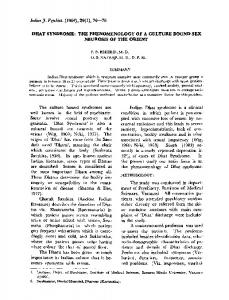
Figure 6: Comparison between the former (left) and revised (right) cluster representation by means of the Team Fortress 2 map Gravelpit. In both cases the coloring of the cluster reflects the weapon usage inside it. Different colors are used for different types of weapon (e.g., orange for sniper rifle, red for rocket launcher). The edges show sniper rifle usage between clusters. the graph whereas the green paths are more widespread. By examining the states visited by the 9-year-olds we could see that they at least tried to collect the bone located in this level (these are the green branches located to the left of the large red branch). However, finding a solution to collect the bone seemed to be too difficult and therefore they opted for other easier solutions (e.g., C) in the end. As can also be seen from the graph, 9-year-olds preferred solution C over solution A, mostly chosen by 8-year-olds. Finally, the nodes along the red branch are larger than the greenish nodes, indicating that 8-year-olds needed more attempts to find a solution (every time a player restarts the level he starts from the beginning and is therefore visiting the same states again).
5.
CLUSTERING
Clustering of states serves two purposes: First, it groups states close to each other and, second, it reduces the visual complexity of the graph. As described in our previous work [29] we currently employ Quality Threshold (QT) clustering [11] using the Euclidean distance between states in the embedding as measure of distance between pairs of states. In case MDS is used to obtain the graph embedding, this also means that similar states (according to the dissimilarity function used for MDS) are grouped together. For example, for the DOGeometry graphs used in the previous section, this would mean that states with a similar arrangement of tiles would be grouped together. The maximum diameter of a cluster and the minimum number of nodes per cluster can be specified by the user. The result of the clustering is a set of k induced subgraphs Gi = (Si , Ai ), Si ⊆ S, Ai = {(u, v) ∈ A : u, v ∈ Si }. Furthermore, Si ∩ Sj = ∅ for any i 6= j. A cluster is there-
fore represented by a meta-node containing the respective subgraph. Please note, that we do not demand the usual S S = ki=1 Si , i.e., nodes must not necessarily belong to a cluster in our case. Actions between states of two different clusters Si and Sj are merged into a single meta-edge em = {(u, v) ∈ A : u ∈ Si , v ∈ Sj }, i 6= j. In the same manner, actions between states inside a cluster Si and a specific state s not belonging to any cluster are combined to a metaedge em = {(u, s) ∈ A : u ∈ Si }. In our previous implementation clusters were represented by the convex hull of their contained states. Clusters could be closed, in which case the contained states and edges were not visible and the convex hull was shrunken by a certain amount or opened in which case the contents were visible and the convex hull had its original size. The color-coding of a cluster polygon reflected the minimum number, maximum number or percentage distribution of state types, action types or player attributes. In case the distribution of an attribute should be displayed, segmented filling of the polygon was used to reflect this distribution. Figure 6 (left) shows an example of this representation. However, feedback indicated that this visual representation was misleading since the polygon size depends on the spatial spread of the state but the color-coding reflects the frequency of a variable. Since area and frequency are highly unlikely to be correlated with each other this can lead to misinterpretation of the amounts. We therefore redesigned the cluster representation (cf. Figure 6 (right) for an example) to address this issue. In the closed condition clusters are now represented as a special node of the graph. The area of the node reflects the sum of the areas of all underlying states. This way clusters with many states or highly visited states are larger than clusters with only a few or less visited nodes. The coloring
of the special node resembles a pie-chart, directly showing the percentage distribution of the attribute in question. Values between clusters can now be compared more easily since all pie-charts are visible at once and must not need to be accessed individually as it was the case in the previous implementation (where the pie-charts were shown as tooltip when the mouse was placed over a cluster). When the cluster is open the same representation as in the previous version is used. This way one can still examine the areal spread of a cluster, whereas the closed circular representation makes comparing values easier. However, clusters may not necessarily be non-overlapping anymore as it was the case in the previous representation. Figure 6 compares the two representations exemplarily by means of the map Gravelpit from the team-based first-person shooter Team Fortress 2 [24]. Nodes show positions where an entity has been killed (gray nodes) or killed another entity (yellow nodes). Actions depict shooting with different kind of weapons. Clustering in this scenario reveals fiercely contested areas. The coloring of the clusters reflects the weapon usage. In both screenshots the cluster located in the middle at the bottom is open and the tooltip for the topmost right cluster is visible. Furthermore, all edges except the ones associated with the sniper rifle (orange) are hidden. This way it is not only possible to observe where a weapon has been used but also where the victim was located. In this example sniper-rifle usage concentrates on the upper part and lower left part of the map. Figure 7 shows another example of clustering, where the coloring of the clusters does not reflect a certain action, but a specific player attribute. The graph shows data from the WoWAH dataset from January, 5, 2009 from 1199 players who have visited the continent Northrend at that day. The clustering reflects the distribution of the different races in the different zones. Since the distribution is roughly the same in each cluster – Blood Elfs (red) constitute the majority in each cluster, followed by Undead (blue) and Tauren (orange) – we can conclude that the different races do not have any preference toward a specific zone. Furthermore, the graph shows migration between the city-state Dalaran and the other zones.
6.
LIMITATIONS AND FUTURE WORK
As discussed in Section 5 we currently use QT clustering to form clusters based solely on their distance and therefore do not take the connectivity between states into account. Graph clustering on the other hand aims to group nodes such that there are many edges within a group but relatively few between them (see, e.g., [22]). In respect to a play-graph such a clustering would focus on actions rather than states and could therefore be an interesting alternative to explore. Other possibilities could be to specify clusters manually or to derive them automatically based on the level geometry. Furthermore, clusters are currently not considered in calculating the difference graph (although clustering can be applied to the resulting difference graph). Since clusters are very likely to be different in the two source graphs (therefore encompassing different subgraphs) they can not be easily subtracted from each other. However, in scenarios where the clusters can be considered to be fixed, like in the World of Warcraft example in Figure 7, calculating the difference between clusters would be reasonable. It should be mentioned, that the difference graph works
Figure 7: Play-graph for the World of Warcraft continent Northrend. The clustering reflects the percentage distribution of the races within the different zones (Orc = yellow, Tauren = orange, Troll = green, Undead = blue, Blood Elf = red) along with migration between Dalaran and the other zones. best if the two graphs to be compared share a large number of nodes with the same labels. If the correspondence is weak – like in the Team Fortress 2 example, where it is highly unlikely that two different entities will ever be at the same state since the position is part of the state definition – the difference will be less significant. We are currently working on including subgraph matching into our system. Subgraph matching (or subgraph isomorphism) is the problem of determining if a larger graph G = (V, E) contains a subgraph which is isomorphic to another graph G0 = (V 0 , E 0 ), with V 0 ⊆ V and E 0 ⊆ E. This would allow the user to look for certain patterns of play (i.e., sequences of actions) in the play-graph. For example, if a developer of a fighting game is interested if players regularly perform a specific combo (like front punch – back punch – front kick) he could input a graph corresponding to this combo and the visualization system would highlight all occurrences of it. Finally, we are currently in the process of performing an evaluation of the visualization with potential users.
7.
CONCLUSIONS
Building upon our previous work on gameplay analysis we introduced the concept of a play-graph as a way to formally describe and decompose gameplay into states, actions and players. In contrast to many other visualizations which have been developed with a specific game in mind, the playgraph formalism can be applied to different types of games. Furthermore, we proposed the use of difference graphs to compute the changes between two datasets. Such a difference graph highlights the areas where player activity has risen or declined. Viewing gameplay as graph allows us to use concepts from the rich field of graph theory and apply them to the understanding of player behavior. One, in our opinion, promising future direction is the use of subgraph isomorphism algorithms to find specific patterns in the collected data.
Based on feedback on our previous prototype we also revised the visual representation of clusters. Instead of representing them with convex polygons, circular nodes are used which at the same time act as pie-charts showing the percentage distribution of a specific attribute. The size of such a node corresponds to the number of combined visits to all states within a cluster rather than on the spatial spread which proofed to be misleading. As proof of concept we applied the play-graph concept to telemetry data from three different games.
8.
[15]
[16] [17]
REFERENCES
[1] E. Andersen, Y.-E. Liu, E. Apter, F. Boucher-Genesse, and Z. Popovi´c. Gameplay analysis through state projection. In Proc. of FDG 2010, pages 1–8. ACM Press, 2010. [2] D. Archambault. Structural differences between two graphs through hierarchies. In Proc. of GI 2009, pages 87–94, Toronto, Ont., Canada, Canada, 2009. Canadian Information Processing Society. [3] D. Archambault, H. C. Purchase, and B. Pinaud. Difference map readability for dynamic graphs. In Proc. of GD 2010, pages 50–61, Berlin, Heidelberg, 2011. Springer. [4] Blizzard Entertainment. World of Warcraft. PC, 2004. [5] J. Dankoff. Game telemetry with playtest DNA on Assassin’s Creed. http://engineroom.ubi.com/game-telemetry-withplaytest-dna-on-assassins-creed-part-3/, Accessed: October, 2012. [6] P. N. Dixit and G. M. Youngblood. Understanding playtest data through visual data mining in interactive 3D environments. In Proc. of CGAMES 2008, 2008. [7] A. Drachen and A. Canossa. Analyzing spatial user behavior in computer games using geographic information systems. In Proc. of MindTrek 2009, pages 182–189. ACM Press, 2009. [8] A. Drachen, A. Canossa, and G. N. Yannakakis. Player modeling using self-organization in Tomb Raider: Underworld. In Proc. of CIG 2009, pages 1–8. IEEE Press, 2009. [9] C. Erten, P. J. Harding, S. G. Kobourov, K. Wampler, and G. V. Yee. GraphAEL: Graph animations with evolving layouts. In G. Liotta, editor, Graph Drawing, volume 2912 of LNCS, pages 98–110. Springer, 2003. [10] A. R. Gagn´e, M. S. El-Nasr, and C. D. Shaw. A deeper look at the use of telemetry for analysis of player behavior in RTS games. In Proc. of ICEC 2011, pages 247–257. Springer, 2011. [11] L. J. Heyer, S. Kruglyak, and S. Yooseph. Exploring expression data: Identification and analysis of coexpressed genes. Genome Research, 9(11):1106–1115, 1999. [12] N. Hoobler, G. Humphreys, and M. Agrawala. Visualizing competitive behaviors in multi-user virtual environments. In Proc. of VIS 2004, pages 163–170. IEEE Computer Society, 2004. [13] K. Isbister and N. Schaffer. Game Usability: Advancing the Player Experience. Morgan Kaufmann, 2008. [14] J. Juul. Introduction to game time. In N. Wardrip-Fruin and P. Harrigan, editors, First
[18]
[19]
[20]
[21]
[22] [23]
[24] [25]
[26]
[27]
[28]
[29]
[30]
[31]
Person: New Media as Story, Performance, and Game, pages 131–141. First edition, 2004. J. H. Kim, D. V. Gunn, E. Schuh, B. Phillips, R. J. Pagulayan, and D. Wixon. Tracking real-time user experience (TRUE): A comprehensive instrumentation solution for complex systems. In Proc. CHI 2008, pages 443–452. ACM Press, 2008. J. B. Kruskal and M. Wish. Multidimensional Scaling. Sage Publications, 1978. Y.-T. Lee, K.-T. Chen, Y.-M. Cheng, and C.-L. Lei. World of Warcraft avatar history dataset. In Proc. of MMSys ’11, pages 123–128. ACM Press, 2011. C. Lewis and N. Wardrip-Fruin. Mining game statistics from web services: a World of Warcraft armory case study. In Proc. of FDG 2010, pages 100–107. ACM Press, 2010. Y.-E. Liu, E. Andersen, R. Snider, S. Cooper, and Z. Popovi´c. Feature-based projections for effective playtrace analysis. In Proc. of FDG 2011, pages 69–76. ACM Press, 2011. B. Medler, M. John, and J. Lane. Data Cracker: developing a visual game analytic tool for analyzing online gameplay. In Proc. of CHI 2011, pages 2365–2374. ACM Press, 2011. J. L. Miller and J. Crowcroft. Group movement in World of Warcraft battlegrounds. Int. J. Adv. Media Commun., 4(4):387–404, Nov. 2010. S. E. Schaeffer. Survey: Graph clustering. Comput. Sci. Rev., 1(1):27–64, Aug. 2007. D. Schoenblum. Zero to millions: Building an XLSP for Gears of War 2. In Game Developer Conference 2010, 2010. Valve Corporation. Team Fortress 2. PC, 2007. Valve Corporation. Half-life 2: Episode two stats. http://www.steampowered.com/status/ep2/ep2_ stats.php, Accessed: October, 2012. Valve Corporation. The science of counter strike: Global offensive. http://blog.counterstrike.net/science/maps.html, Accessed: October, 2012. G. Wallner and S. Kriglstein. Design and evaluation of the educational game DOGeometry - a case study. In Proc. ACE 2011, pages 14:1–14:8. ACM Press, 2011. G. Wallner and S. Kriglstein. Dogeometry: teaching geometry through play. In Proc. FnG 2012, FnG ’12, pages 11–18, New York, NY, USA, 2012. ACM Press. G. Wallner and S. Kriglstein. A spatiotemporal visualization approach for the analysis of gameplay data. In Proc. CHI 2012, pages 1115–1124, New York, NY, USA, 2012. ACM Press. D. Williams, N. Yee, and S. E. Caplan. Who plays, how much, and why? Debunking the stereotypical gamer profile. Journal of Computer-Mediated Communication, 13(4):993–1018, 2008. G. Zoeller. Development telemetry in video games projects. In Game Developer Conference 2010, 2010.