Playing with Partial Knowledge in Membrane Systems: A Logical Approach Matteo Cavaliere1 and Radu Mardare2 1
Microsoft Research – University of Trento Centre for Computational and Systems Biology, Trento, Italy
[email protected] 2 D.I.T., University of Trento Trento, Italy
[email protected]
Abstract. We propose a logic for specifying and proving properties of membrane systems. The main idea is to approach a membrane system by using the “point of view” of an external observer. Observers (treated as epistemic agents) accumulate their knowledge from the partial information they collect by observing subparts of the system and by applying logical reasoning to this information. We provide a formal framework to combine and interpret distributed knowledge in order to recover the complete knowledge about a membrane system. The proposed logic can be used to model biological situations where information concerning parts of the biological system is missing or incomplete.
1
Motivations
Abstracted as multi-agent system, a biological system can be seen as an interactive, concurrent and distributed system with a rather complex behavior. The success in dealing with this complexity depends on the mathematical model chosen as abstraction of the system. Consider, for example, the immune system [2]. This is constituted by a network of cells, tissues and organs that work together to defend the body against attacks by foreign invaders - microbes, germs, bacteria, viruses, parasites, etc. The immune system’s job is to keep them out or, failing that, to seek out and destroy them. The immune system functions due to an elaborate and dynamic communications network. Millions of cells, organized into sets and subsets, gather in clouds swarming around a hive and pass information back and forth. Suppose now that we are interested in modelling the interaction of our body with a given virus. Excepting the immune system, our body contains also other subsystems, but we can decide that, for the given situation, all the other parts are meaningless. So we decide to ignore them. For instance, if we consider the case in which the virus is already present in our body, the first approximation of the biological reality will consider a main system (our body) in which are
Playing with Partial Knowledge in Membrane Systems
243
present two subsystems - the virus and the immune system. Going deeper, the first interaction between the two subsystems involves the innate immune system, which is just a subsystem of the immune system comprised of hereditary components that provide an immediate “first-line” of defense to continuously ward off pathogens. This subsystem is able to annihilate “well-known” viruses. If this is the real situation, then modelling only the innate immune system in relation with the virus is enough for comprehending the biological phenomenon. But if the virus is unknown, then we might need to go deeper with modelling and, in addition to the innate immune system, to model also phagocytic cells. These are cells that represents the “second-line” of defense for our body. They can analyze unknown entities, destroy viruses and learn the structures of the destroyed entities. In particular, the immune system is able to design special cells for fighting with peculiar types of viruses. Hence, on this level, the modelling have to be more specific representing also other subsystems of the immune system. Depending on the complexity of the biological properties we want to consider, we can go as deep as necessary with representing the biological entities involved. More complex models provide more accurate information. Still, as the costs of modelling and simulation grows with complexity of the model, we have to find the right level of abstraction that gives, with acceptable costs, the information we are looking for. Observe that in biology, as in all the empirical sciences, we cannot hope to reach the level of having complete information concerning a biological phenomenon. Thus, no matter how complex is the model we choose, there exists always properties requiring a bigger complexity. In other words, we always work with partial (observed) knowledge about biological systems and based on this incomplete information we model or simulate biological phenomena. In this paper we show how it is possible to manage incomplete information concerning membrane systems. The work done here can be seen as related to [9] where a formal observer has been introduced to investigate the formal behavior of a membrane system. However in [9] the observer was a mapping assigning a “meaning” to the configurations reached during the evolution of the observed system. In this paper the observer is an epistemic agent: in this way it is possible to analyze situations in which the knowledge about the observed system can also be partial, incomplete or missing.
2
Formal Language Preliminaries
Membrane systems are based on formal language theory and multiset rewriting. We now briefly recall the basic theoretical notions used in this paper. For more details the reader can consult standard books, such as [10] and the corresponding chapters of the handbook [18]. Given the set A we denote by |A| its cardinality and by ∅ the empty set. We denote by N and by R the set of natural and real numbers, respectively. As usual, an alphabet V is a finite set of symbols. By V ∗ we denote the set of all strings over V . By V + we denote the set of all strings over V excluding
244
M. Cavaliere and R. Mardare
the empty string. The empty string is denoted by λ. The length of a string v is denoted by |v|. The concatenation of two strings u, v ∈ V ∗ is written uv. A multiset is a set where each element may have a multiplicity. Formally, a multiset over a set V is a map M : V → N, where M (a) denotes the multiplicity of the symbol a ∈ V in the multiset M . For multisets M and M 0 over V , we say that M is included in M 0 if M (a) ≤ 0 M (a) for all a ∈ V . Every multiset includes the empty multiset, defined as M where M (a) = 0 for all a ∈ V . The sum of multisets M and M 0 over V is written as the multiset (M + M 0 ), defined by (M + M 0 )(a) = M (a) + M 0 (a) for all a ∈ V . The difference between M and M 0 is written as (M −M 0 ) and defined by (M −M 0 )(a) = max{0, M (a)− M 0 (a)} for all a ∈ V . We also say that (M + M 0 ) is obtained by adding M to M 0 (or viceversa) while (M − M 0 ) is obtained by removing M 0 from M . For example, given the multisets M = {a, b, b, b} and M 0 = {b, b}, we can say that M 0 is included in M , that (M +M 0 ) = {a, b, b, b, b, b} and that (M −M 0 ) = {a, b}. If the set V is finite, e.g. V = {a1 , . . . , an }, then the multiset M can be explicitly described as {(a1 , M (a1 )), (a2 , M (a2 )), . . . , (an , M (an ))} where (a, M (a)) can be also written as aM (a) . The support of a multiset M is defined as the set supp(M ) = {a ∈ V | M (a) > 0}. A multiset is empty (hence finite) when its support is empty (also finite). A compact notation can be used for finite multisets: if M = {(a1 , M (a1 )), (a2 , M (a2 )), . . . , (an , M (an ))} is a multiset of finite support, then the string w = M (a ) M (a ) a1 1 . . . an n (and all its permutations) precisely identify the symbols in M and their multiplicities. Hence, given a string w ∈ V ∗ , we can say that it identifies a finite multiset over V , written as M (w), where M (w) = {a ∈ V | (a, |w|a )}. For instance, the string bab represents the multiset M (w) = {(a, 1), (b, 2)}, that is the multiset {a, b, b}. The empty multiset is represented by the empty string λ.
3
Membrane Systems with Symbol-Objects
We recall the basic notions of membrane systems (also called P systems) with symbol-objects. The reader can find further details in the monograph [3]. An updated bibliography of the field can be found at the P systems web-page [1]. Definition 3.1 (Membrane system with symbol-objects). Given a finite set of objects O and an infinite set of labels Lab, we consider the following family of constructs P = {(µ, wj1 , wj2 , · · · , wjm , Rj1 , Rj2 , · · · , Rjm ) | ji ∈ Lab, for i = 1..m}. where – µ is a membrane structure consisting of m membranes arranged in an hierarchical structure enclosed in a main membrane, called skin membrane. The skin membrane separates the system from the surrounding environment; the
Playing with Partial Knowledge in Membrane Systems
245
membranes (and hence the regions that they delimit/enclose) are injectively labeled over the finite set LabΠ = {j1 , j2 , · · · , jm } ⊂ Lab; we convey to label by j1 the skin membrane. – wj1 , wj2 , · · · , wjm are strings that represents multisets over O associated with regions j1 , j2 , · · · , jm , respectively. – Rj1 , Rj2 , · · · , Rjm are finite sets of evolution rules over O, associated to regions j1 , j2 , · · · , jm , respectively. An evolution rule is of the form u → v, where u is a string over O and v is a string over {ahere , aout | a ∈ O} ∪ {ainj | a ∈ O, j ∈ LabΠ }. The symbols here, out, inj , j ∈ Lab are called target indications. To simplify the notation the target indication here is omitted. An element Π = (µ, wj1 , wj2 , · · · , wjm , Rj1 , Rj2 , · · · , Rjm ) ∈ P is called membrane system with symbol-objects, of degree m. We denote by 0 the membrane system of degree 0. We call atomic membrane system a membrane system of degree 1; if its unique membrane (which is also the skin membrane) is labelled by i and to region i is associated the multiset w ∈ O∗ , then we denote it by [w]i . Given a membrane system Π, an evolution of Π is a sequence of membrane systems hΠ0 , Π1 , Π2 , · · · i where Π0 = Π and, for i ≥ 0, each Πi+1 is obtained by applying, to one of the regions of Πi , one of the associated evolution rules. Rule and region are chosen in a non-deterministic manner. The remainder of the system Πi (objects not involved in the application of the rule, set of rules, membrane structure, labelling of the membranes) is left unchanged in Πi+1 . The passage from Πi to Πi+1 using the rule r in region j of Πi is called rj transition and is denoted by Πi −→ Πi+1 . 3 The application of an evolution rule r : u → v ∈ Rj in the region j ∈ LabΠ means to remove the multiset of objects identified by u from region j, and to add the objects specified by the multiset v, in the regions specified by the target indications associated to each object in v. In particular, if v contains an object a with target indication here, then the object a will be placed in the region jr where the evolution rule has been applied. If v contains an object a with target indication out, then the object a will be moved to the region immediately outside the region j (this can be the environment if the region where the rule has been applied is the skin membrane). If v contains an object a with target indication ini , with i ∈ Lab, then the object a is moved from the region j and placed into the region i (this can be done only if such region i exists and is immediately inside region j; otherwise the evolution rule u → v cannot be applied). We call membrane structure contained into membrane j in Π, the membrane structure contained in region j of Π. Definition 3.2 (Membrane composition). Let Π = (µ, wj1 , wj2 , · · · , wjm , Rj1 , Rj2 , · · · , Rjm ) 3
The reader familiar with membrane systems can notice that we use a sequential semantics: at each step only an unique rule is executed once. Actually the logic proposed in this paper is very general and can be extended easily to other semantics, e.g., the maximal parallel one.
246
M. Cavaliere and R. Mardare
be a membrane system and i ∈ Lab − LabΠ . We denote by [Π]i the membrane system Π 0 = (µ0 , wk1 , wk2 , · · · , wkm+1 , Rk1 , Rk2 , · · · , Rkm+1 ) such that – µ0 is µ enclosed into an external membrane labelled by i; the labelling of the membranes of µ is preserved in µ0 ; – k1 = i and ks = js−1 for s = 2..m + 1; consequently wjs = wks−1 and Rjs = Rks−1 ; – wi = λ, Ri = ∅. Example 3.1. Consider the membrane system Π defined by µ = [ [ ]2 ]1 ; R1 = {a → b}; R2 = {b → c}; w1 = b; w2 = a. Then [Π]3 is the system Π 0 defined by µ0 R10 R20 R30 w10 w20 w30
= [ [ [ ]2 ]1 ]3 ; = R1 = {a → b}; = R2 = {b → c}; = ∅; = w1 = b; = w2 = a; = λ.
Definition 3.3 (Parallel composition). Let Π = (µ, uj1 , uj2 , · · · , ujm , Rj1 , Rj2 , · · · , Rjm ) and Π 0 = (µ0 , vk1 , vk2 , · · · , vkn , Rk1 , Rk2 , · · · , Rkn ) be two membrane systems such that j1 = k1 , LabΠ ∩ LabΠ 0 = {j1 } and Rj1 = Rk1 . We call parallel composition of the two systems, denoted by Π|Π 0 , the membrane system Π 00 = (µ00 , wl1 , wl2 , · · · , wlm+n−1 , Rl1 , Rl2 , · · · , Rlm+n−1 ) defined by: – µ00 is obtained by enclosing into a common external the membrane structures contained into the skin membranes of µ and µ0 ; – in µ00 the labelling of the membranes in µ and in µ0 is preserved; the skin membrane of Π 00 is labelled by l1 = j1 = k1 ;
Playing with Partial Knowledge in Membrane Systems
– wl1 = uj1 vk1 .
247
4
The intuition behind the parallel composition operator is that it can be used to divide an entire membrane system in subsystems, where each subsystem can be recognized/understood by a certain external observer. Example 3.2. Consider the membrane systems Π: µ = [ [ ]2 [ ]3 ]1 w1 = ab w2 = cd w3 = aa R1 = {a → b, a → c} R2 = {cd → a} R3 = {a → b, a → d}
Π0 : µ0 = [ [ [ ]5 ]4 ]1 w1 = ee w4 = ccd w5 = a R1 = {a → b, a → c} R4 = {d → c} R5 = {a → b}
Then Π|Π 0 is the system Π 00 defined as µ00 w1 w2 w3 w4 w5 R1 R2 R3 R4 R5
= [ [ ]2 [ ]3 [ [ ]5 ]4 ]1 = eeab = cd = aa = ccd =a = {a → b, a → c} = {cd → a} = {a → b, a → d} = {d → c} = {a → b}.
Let denote by Pi the class of membrane systems having the skin membrane labelled by i. Then it is easy to see that the following theorem holds. Theorem 3.1. (Pi , |, [0]i ) is an Abelian monoid. Also the following theorem can be easily proved. Theorem 3.2. Any membrane system can be composed, by iterating parallel and membrane composition, starting from atomic membrane systems. 4
The definition is correct as LabΠ ∩ LabΠ 0 = {j1 }. Notice that, since the labelling of the membranes is preserved, we have that for s ∈ {1, · · · , m + n − 1} Rls is preserved as in the original system (Π or Π 0 ) and for s 6= 1, wls = uks (wls = vks ) is preserved as in the original system Π (Π 0 , respectively)
248
M. Cavaliere and R. Mardare
Example 3.3. Consider the membrane system Π presented in Example 3.2. The system Π can be obtained as [ [cd]2 ]1 |[ [aa]3 ]1 |[ab]1 with R1 , R2 and R3 as in Π. Clearly [cd]2 , [aa]3 , [ab]1 are atomic membrane systems.
Partial Information in Membrane Systems We want to propose a formal way of playing with partial information about a (membrane) system in order to decide some global properties. The idea is to formally describe open systems. An open system for an observer is a system formed by a known subsystem and an unknown (opened) part about which the observer does not know anything. So if the observer knows a subsystem S1 of a bigger system 5 S1 |S2 , then the observer considers as entire system , any structure of type S1 |S3 , for any possible system S3 . Hence, the properties that the observer knows about the entire system are the properties that systems “like” S1 |S2 , S1 |S3 , etc. have in common. Consider again the example, presented in the Introduction, where a virus attacks our body. We have decided to model a relevant part of immune system, say I, in relation with the virus v. Hence the model of a body that has been penetrated by a virus is body = I|v|S, where S denotes the rest of the body (we have not considered to model the rest of the body in details since the system I is enough for comprehending the interaction with the virus). Suppose now that the properties we try to specify do not concern only the subsystem I|v (the one we have considered) but the whole body I|v|S. Can we sustain that each property of the system I|v can be stated about the whole body I|v|S? For correctly answering to this question, we propose a logic to play with partial information. Consider a complex biological system about which we have only partial information. This information is collected by some observers placed in different points of the system. Each observer analyzes a subsystem. Our logic develops the framework needed to combine the knowledge of these observers such that is possible to derive interesting properties about the whole system, even without having complete information about it. Playing with observers might cost less than fully investigating the system and it might provide enough information for deciding on the properties we are interested in. All depends on how we place the observers and how we combine their knowledge in deriving complex properties. Formally, we propose a logic developed in dynamic-epistemic paradigm [11] and enriched with operators from spatial logics [5, 4, 7, 8]. We call it dynamic 5
We use the parallel operator to describe the situation of two concurrent systems forming, together, an upper-system.
Playing with Partial Knowledge in Membrane Systems
249
epistemic spatial logic. The syntax allows to express open systems and the knowledge of observers. By combining the knowledge of different observers we can specify and verify complex properties about the whole system without having complete knowledge about it. In related papers [15, 16, 14] has been proposed Hilbert-style axiomatic systems for different such logics, and there have been proved that they are decidable against a semantics based on process algebra, even in the cases for which the classical spatial logics have been proved to be undecidable [6].
4
Playing with Partial Information
In this section we will show how, playing with partial information about a system, we can derive properties of the whole system. For this we reconsider a popular example used in epistemic reasoning [11] adapted for a biologically inspired situation. Consider a biological system S composed by four disjoint subsystems S = S1 |S2 |S3 |S4 . In Figure 1 there are four cells S1 , S2 , S3 and S4 . Each cell contains a vacuole that can be either normal, having an oval shape as in S3 , S4 , or abnormal having a non-circular shape as the vacuoles of S1 and S2 . Suppose, in addition, that the system is analyzed by four observers, each observer having access to only a subpart of S. Thus observer O1 can see the subsystem S2 |S3 |S4 , O2 the subsystem S3 |S4 |S1 , O3 can see the subsystem S4 |S1 |S2 and observer O4 sees S1 |S2 |S3 . Each observer has a display used for making public announcements.
Fig.1: The system S
Fig.2: The perspective of O1
The observers know that the system S contains abnormal vacuoles and each observer tries to compute the exact number of them and their positions in the system. In doing this the observers do not communicate but only witness the public announcements. Each observer displays 0 until it knows the exact number and positions of abnormal vacuoles, moment in which it switches to 1. In addition, the observers are synchronized by a clock that counts each step of computation. Hence, after each “tick” the observer has to evaluate its knowledge and
250
M. Cavaliere and R. Mardare
to decide if its display remains on 0 or switches to 1. Thus each observer computes information about the whole system by using the partial information it possesses and by evaluating the knowledge of the other observers (by reading their displays). If an observer is able to decide the correct number of abnormal vacuoles and their exact positions in the system, then it succeeded to do this with a lower cost than the cost needed for fully investigating the system. Hereafter we show that such a deduction is possible. Consider that the real state of the system is the one in Figure 1 and suppose that we can control only the observer O1 . As O1 sees the subsystem S2 |S3 |S4 , it sees an abnormal vacuole in subsystem S2 and normal vacuoles in S3 and S4 ; in Figure 2 it is represented the perspective of O1 . But it does not know if the system S1 has a normal or an abnormal vacuole. For O1 both situations are equally possible. Hence, after the first round of computation the display of O1 remains to 0. As it concerns observer O2 , it sees an abnormal vacuole, in S1 , but it doesn’t know what is in S2 , thus, after the first round, it will show 0 too.
Fig.3: A hypothetical perspective of O2
Fig.4: The real perspective of O2
It starts the second round of computation. We come back to our observer, O1 . The observer has seen that, after the first round, the observer O2 has not succeed to understand the situation (as O2 shows 0 on its display). If the system S1 would contain a normal vacuole then in the first round O2 would have seen only normal vacuoles, as in Figure 3. O2 also knows that there is at least one abnormal vacuole. Hence, if this was the case, O2 had enough information to decide, in the first round, that the only abnormal vacuole of the system is in S2 . Consequently 1 had to appear on its display. But this was not the case (O1 can see that by looking to the display of O2 ). This means that what O2 observed was the situation presented in Figure 4. Therefore it is possible to decide that the real situation of the system is the one with an abnormal vacuole in S1 . Thus using only O1 it is possible to compute the real configuration of the system and then O1 will display 1. The example works similarly in more complex situations. Observe the advantages of this analysis: using only the partial information available to O1 about the system S and judging the behavior of the other observers, we were able to compute the real configuration of the system. The ob-
Playing with Partial Knowledge in Membrane Systems
251
servers do not exchange information about S, but only about their level of understanding (their observations of) S. The rest can be computed. If each subsystem is very complex, and usually this is the case in biology, then the complete information about the system can be larger than an observer can store or manipulate. Note also that the observers do not need a central unit for organizing their information. Each observer organizes its own information and makes public announcements about its level of knowledge. They work simultaneously in a distributed network and only playing with their partial information about S and with the information about the state of the network are able to derive overall properties of the system. The approach fits well with the real situation of biological systems. We work always with partial information which are collected by some observers as results of “measuring” different aspects of a biological phenomena. Sometimes these different ”faces” of the same phenomena cannot be integrated in the same mathematical model, or seeking for a property might involve evaluation of different models. For such situations, a formalized way for automatically reasoning, as in the previous example, might help. Hereafter we introduce a logic designed for this purpose.
5
A Logic of Partial Information
As pointed in the previous section, the role of observers in understanding and manipulating biological information is significant. We present a logic of observers, called dynamic epistemic spatial logic [15, 17, 16, 14], developed for specifying and model-checking properties of multi-agent systems. It can be successfully applied for analyzing membrane systems. Our logic proposes a formal way of combining and analyzing the information provided by different observers about the same biological phenomena. Our logic can be related with spatial logics [4, 5, 7, 8]. For a detailed presentation of it and for a Hilbert-style axiomatization the reader is referred to [15, 17, 16, 14]. 5.1
The Syntax of LObs
Suppose that we have a class Obs of observers ranged over by A, B, C. We enrich the language of propositional logic with knowledge operators indexed by observers KA . A statement like KA φ is read “observer A knows φ”. Then we can compose more complex epistemic statements. Thus “observer A1 knows that observer A2 knows φ” is formalized by KA1 KA2 φ. A formula like KA φ∧KA (φ → ψ) → KA ψ is interpreted as “if observer A knows φ and φ → ψ then the observer knows ψ”. In addition to these operators we add some spatial operators meant to describe the spatial distribution of the subsystems. Anticipating the semantics, we present the intuition behind these operators.
252
M. Cavaliere and R. Mardare
Formula 0 is meant to characterize the trivial membrane system 0 that might be ignored in a complex situation6 . Inspired by spatial logics [5, 7, 8], we introduce the parallel operator φ k ψ meant to express the situation in which our system can be decomposed in two (parallel) subsystems, one satisfying φ and the other one satisfying ψ. > will be satisfied by any system, hence it expresses consistency, ”true“. The role of this element of syntax is essential in expressing open systems. As > is a property that characterizes any system, φ k > characterizes any system that has a subsystem satisfying φ and the rest of the system is, possibly, unknown. By negation, ⊥ will be used to express the inconsistency. We also design operators to express membranes. Thus JφKi is a property that characterizes a membrane system [Π]i where Π is a membrane system that has the property φ. Similarly we introduce a formula JwKi that characterizes the atomic membrane system JwKi . As we propose a logic for the studying of membrane systems together with their evolutions, we allow some modal operators indexed by the transitions of the systems to express the evolutions of a membrane system. Thus hri iφ is an operator meant to specify the system Π able to perform a transition labelled by ri ri (in short, transition ri ), i.e. Π −→ Π 0 , and Π 0 satisfies φ. These operators are characteristic for dynamic logics [12] and are basic operators in Hennessy-Milner logic [13]. Formally, the language of dynamic epistemic spatial logic LObs is defined as follows: Definition 5.1 (The language). Let Obs be the set of observers, O an alphabet and Lab a set of labels. We define the language of dynamic epistemic spatial logic, by the following grammar: φ := 0 | > | ¬φ | φ ∧ φ | JwKi | JφKi | φ k φ | hri iφ | KA φ
where A ∈ Obs, w ∈ O∗ , i ∈ Lab and r is a rule of the set Ri .
Definition 5.2 (Derived operators). In addition we introduce some derived operators, widely used in dynamic-epistemic logics: def
1. ⊥ = ¬> def
2. φ ∨ ψ = ¬((¬φ) ∧ (¬ψ)) def
3. φ → ψ = (¬φ) ∨ ψ def
4. [ri ]φ = ¬(hri i(¬φ)) def
5. 1 = ¬((¬0) k (¬0)) ∼
def
6. K O φ = ¬KO ¬φ 6
Some syntaxes of classical logic use 0 for denoting false. This is not the case here. We use ⊥ to denote false.
Playing with Partial Knowledge in Membrane Systems
253
The dynamic modality [ri ]φ, the dual operator of hri iφ, captures the weakest precondition of a transition ri of a membrane system w.r.t. a given postspecification φ. We have used the square brackets to denote it, as this notation is classical in dynamic logics (inspired by the box operator of modal logic). It shouldn’t be confused with the same brackets use on membrane systems for denoting membrane composition. Formula 1 is meant to describe the situation in which the system cannot be decomposed into two non-trivial subsystems.
5.2
The Semantics of LObs
In this subsection we introduce a semantics for the presented logic. It will be defined underpinning on a satisfiability relation Π |= φ, that establishes the condition under which we can affirm that the membrane system Π has (satisfies) the property φ. As introduced earlier, each observer sees a membrane system in P. This membrane system is the “structure” that the observer can recognize in any more complex system. Hence, for introducing the semantics, we have to devise an interpretation function int : Obs −→ P that associates to each observer A ∈ Obs a membrane system int(A) = Π that represents the system that the observer is able to “recognize”. The intuition is to define the knowledge of the observer A as the common properties of all systems where A is active, i.e., systems that contains Π as subsystem. Definition 5.3 (Models and satisfaction). Given a class Obs of observers and an interpretation function int : Obs −→ P we introduce the satisfaction relation by: Π |= > always Π |= ¬φ iff Π 2 φ Π |= φ ∧ ψ iff Π |= φ and Π |= ψ Π |= φ k ψ iff Π = Π1 |Π2 and Π1 |= φ, Π2 |= ψ Π |= 0 iff Π = 0 Π |= JwKi iff Π = [w]i Π |= JφKi iff Π = [Π 0 ]i and Π 0 |= φ ri Π |= hri iφ iff there exists a transition Π −→ Π 0 and Π 0 |= φ 0 0 Π |= KA φ with int(A) = Π iff Π = Π |Π 00 and ∀Π 0 |Π 000 ∈ P we have 0 Π |Π 000 |= φ Then the semantics of the derived operators can be obtained. ri Π |= [ri ]φ iff for any Π 0 such that Π −→ Π 0 (if any), Π 0 |= φ 0 00 Π |= 1 iff there are no systems Π , Π with Π = Π 0 |Π 00 and Π 0 6= 0 6= Π 00 ∼
Π |= K A φ for int(A) = Π 0 iff either Π 6= Π 0 |Π 00 for any Π 00 , or it exists 0 Π |Π 000 such that Π 0 |Π 000 |= φ
254
5.3
M. Cavaliere and R. Mardare
Expressivity
Open systems: We can exploit the use of > to express properties of open membrane systems. By an open membrane system we mean a system for which we know only a subpart and we accept any upper-system of the known part as possible configuration for the overall situation. For example if our system is Π = Π1 |Π2 and an observer knows only Π1 , then for the observer any system of type Π1 |Π3 , for any Π3 ∈ P, is a possible system Π. Hence what is outside Π1 is “open information” for our observer. Reconsidering the example in section 4, for A1 , in the initial state, Π was an open system because Π1 has (for A1 ) either a normal, or an abnormal vacuole. If we want to express that a system Π is an open system containing a known subsystem Π1 then we can express this by allowing an observer A1 ∈ Obs to see only Π1 , i.e. int(A1 ) = Π1 . Then Π |= KA1 > means that the system Π is an upper system of Π1 . Indeed, by our semantics, this means that Π = Π1 |Π2 and for any Π3 ∈ P we have Π1 |Π3 |= >. But the last condition is trivially true, hence the semantics is equivalent to Π = Π1 |Π2 , where Π2 can be any system. Due to this, we can use KA1 > to say ”in this system Π1 is a subsystem”. We can be more specific and express that any upper system of Π1 has the property φ. We can do this by taking an upper system of Π1 , say Π = Π1 |Π2 , and stating that Π |= KA1 φ, where int(A1 ) = Π1 . This is equivalent with saying that for any Π3 ∈ P we have Π3 |Π1 |= φ. If we can characterize a membrane system up to identity, we can express that a system Π is an open system containing a known subsystem characterized by φ also without using the epistemic operator, by Π |= φ k >. Indeed, w.r.t. our semantics this means that Π = Π1 |Π2 and Π1 |= φ, Π2 |= >. As φ satisfies the known system and > can be stated about any system Π3 ∈ P we obtain that any system of type Π1 |Π3 , for any Π3 ∈ P satisfies φ k >. Characteristic formulas: Using our logic we can define formulas that will fully identify a membrane system. Recall that Theorem 3.2 states that each membrane system can be decomposed, by using parallel and membrane composition, in atomic membrane systems. We show further how, by induction in top of atomical membrane systems, we can define characteristic formulas for any membrane system. A characteristic formula of a membrane system Π have to be a formula of our logic φΠ such that – Π |= φΠ – if Π 0 |= φΠ then Π 0 = Π We define such formulas inductively on structure of Π. def
1. φ0 = 0 def
2. φ[w]i = JwKi
def
3. φΠ|Π 0 = φΠ k φΠ 0 def
4. φ[Π]i = JφΠ Ki
Theorem 5.1. Being a membrane system Π, the formula φΠ is a characteristic formula for it.
Playing with Partial Knowledge in Membrane Systems
255
The fact that we can define characteristic formulas for membrane systems open the possibility to project any semantical problem in syntax. Thus, if we want to verify that the process Π has a property ψ, i.e. Π |= ψ, we can project this problem in syntax where it is equivalent with ` φΠ → ψ, where we denoted by φΠ the characteristic formula of Π as before. Now the problem Π |= ψ is equivalent with proving φΠ → ψ with the axioms of our logic. Similarly, we can express the fact that between Π and Π 0 there exists a ri Π 0 by stating ` φΠ → hri iφΠ 0 . Now ` φΠ → hri iφΠ 0 can be transition Π −→ ri Π 0 exists. On this direction we proved from the axioms iff the transition Π −→ can also imagine more complex situations. Consider, for example, that we have the system Π and we want to know if, after doing the transitions labelled by ri then sj , ts will reach a state (i.e., a membrane system) that will have a subpart satisfying ψ. This can be syntactically said by ` φΠ → hri ihsj ihts i(ψ k >). Indeed ψ k > describes a system having a subsystem that satisfies ψ. Then the dynamic operators prefixing it, hri ihsj ihts i(ψ k >), means that the system will reach the state satisfying ψ k > only after it performs the transitions labelled by ri , sj , ts in this order. Validity: The presented syntax allows to express the validity of a property in a class of membrane systems having the same external membrane i, i.e. the property is satisfied by any of these systems. We can do this by using a “blind observer ”, i.e. an observer A0 ∈ Obs that sees only the trivial system embedded in i, int(A0 ) = [0]i . Indeed, the epistemic operator KA0 has an interesting semantics: Π |= KA0 φ iff for any Π 00 ∈ Pi we have Π 00 |= φ. This is so because, if a system Π has the property KA0 φ then φ is satisfied by any system Π 0 ∈ P that can be decomposed in Π 0 = [0]i |Π 00 , i.e. Π 0 must have the skin membrane i, hence Π 0 ∈ Pi . But Π 0 has the property Π 0 |[0]i = Π 0 , as [0]i is the null element of the monoid (Pi , |). Hence φ is satisfied by any system with the skin i, i.e. it is a valid property over Pi . Thus we can encode, in syntax, the validity of a property. Consequently, KA0 > is a validity, as [0]i is a subsystem of any system in Pi , Π = Π|[0]i . Satisfiability: Also the satisfiability of a property can be encoded in the syntax. We say that a property is satisfiable if it exists at least one membrane system having this property. For this purpose we use the dual of the knowledge operator ∼
for the blind observer, K A0 . ∼
Π |= K A0 φ iff it exists a membrane system Π 00 ∈ Pi such that Π 00 |= φ ∼
Indeed, if a system Π satisfies K A0 φ then either Π 6= Π 0 |[0]i (this is not the case as always Π = Π|[0]i ) or it exists Π 00 such that Π 00 |[0]i |= φ. But Π 00 |[0]i = Π 00 , ∼
hence it exists a system Π 00 ∈ Pi that satisfies φ and vice versa. Thus K A0 φ provides a way to encode, in syntax, the satisfiability of a property.
256
5.4
M. Cavaliere and R. Mardare
(Some) Axioms and Theorems
In [15, 17, 16, 14] it has been introduced a Hilbert-style axiomatic system for dynamic epistemic spatial logic. We present further some interesting axioms and theorems that can offer an idea about what can be specified and proved using our logic. Axiom E 1 ` JφKi k J0Ki ↔ JφKi The previous axioms states that an empty membrane system contained in membrane i do not come with extra properties if it is considered as a subsystem of a system having the skin i. Hence, such a subsystem is ”transparent“. Axiom E 2 ` (hri iφ) k ψ → hri i(φ k ψ). If a subsystem Π1 of a system Π = Π1 |Π2 can do a transition ri and further it satisfies φ while its counterpart Π2 satisfies ψ, then the system Π can be described as able to perform a transition ri thus passing to a system satisfying φ k ψ. Axiom E 3 ` KA φ ∧ KA (φ → ψ) → KA ψ This axiom E3 is the classical (K)-axiom stating that our epistemic operator is a normal one. It states that if an observer A knows φ and that φ → ψ then it knows ψ. It is an usual axiom of knowledge [11]. Axiom E 4 ` KA φ → φ Also this axiom is classic in modal and epistemic logics - the axiom (T) necessity axiom. It states that the knowledge of any observer must be true, i.e. an observer cannot know something that is not true. Axiom E 5 ` KA φ → KA KA φ. Also axiom E5 is well known in epistemic logics. It states that our epistemic agents (observers) have the positive introspection property, i.e. if an observer A knows something then it (i.e., the observer) knows that it knows that thing. Axiom E 6 ` KA > → (¬KA φ → KA ¬KA φ) Axiom E6 states a variant of negative introspection, saying that if an observer A is active (the system that the observer knows is a subsystem of the whole system) and if the observer does not know φ, then the observer knows that does not know φ. Negative introspection is also present in classic epistemic logics. Rule ER 1 If ` φ then ` KA > → KA φ.
Playing with Partial Knowledge in Membrane Systems
257
Rule ER 1 states that any active observer knows all the tautologies. Also in this case we deal with a well known epistemic rule, widely spread in epistemic logics. But our rule works under the assumption that the observer is active. In [15, 17, 16, 14] we present a full axiomatic system and we prove many theorems inside it. Hereafter we will sketch some soundness proofs for the previous axioms to clarify the intuitions that motivates the choice of them. Similarly all the axioms can be proved to be sound. Theorem 5.2 (Soundness of axiom E2). |= (hri iφ) k ψ → hri i(φ k ψ) Proof. If Π |= (hri iφ) k ψ, then Π = Π1 |Π2 , Π1 |= hri iφ and Π2 |= ψ. So ri ri Π 0 = Π10 |Π2 and Π 0 |= φ k ψ. Π10 and Π10 |= φ. So ∃Π = Π1 |Π2 −→ ∃Π1 −→ Hence Π |= hri i(φ k ψ). Theorem 5.3 (Soundness of axiom E3). |= KA φ ∧ KA (φ → ψ) → KA ψ Proof. Suppose that Π |= KA φ and that Π |= KA (φ → ψ), where int(A) = Π1 . Then Π = Π1 |Π2 and for any Π 0 we have Π1 |Π 0 |= φ and Π1 |Π 0 |= φ → ψ. Hence for any such Π1 |Π 0 we have Π1 |Π 0 |= ψ and because Π = Π1 |Π2 we obtain that Π |= KA ψ. Further we present some meaningful theorems that can be derived with our system. Theorem 5.4. ` KA φ → KA >. This theorem says that an observer knows something only if it is active. Theorem 5.5 (Monotonicity of knowledge). If ` φ → ψ then ` KA φ → KA ψ The knowledge is monotone, meaning that if a property φ guarantees a property ψ then any observer that knows φ knows also ψ. Theorem 5.6 (Consistency of knowledge). ` KA φ → ¬KA ¬φ. This theorem states that the knowledge of an observer is always consistent; the observer cannot know φ and ¬φ. Theorem 5.7 (Ontological dependency). If int(A) = Π1 |Π2 , int(A1 ) = Π1 then ` KA > → KA1 >. If the system associated to observer A1 is a subsystem of the system associated to observer A, then the activation of observer A implies the activation of observer A1 . For more interesting theorems, the reader is referred to [15, 17, 16, 14], where, for this logic, it is also developed a semantics on process algebras proved to be sound and complete against the same axiomatic system.
258
6
M. Cavaliere and R. Mardare
A (Simple) Case Study
Consider the membrane systems defined as: Π: µ = [ [ ]2 [ ]3 [ ]4 ]1 w1 = λ w2 = a w3 = b w4 = c R1 = {r0 : b −→ bin4 } R2 = {r00 : a −→ bout } R3 = {r000 : b −→ aout } R4 = {rIV : b −→ cout }
Π0 : µ0 = [ [ ]2 [ ]3 ]1 w1 = λ w2 = a w3 = b
Π 00 : µ00 = [ [ ]4 ]1 w1 = λ w4 = c
R1 = {r0 : b −→ bin4 } R2 = {r00 : a −→ bout } R3 = {r000 : b −→ aout }
R1 = {r0 : b −→ bin4 } R4 = {rIV : b −→ cout }
Obviously Π = Π 0 |Π 00 . Suppose now that we have an observer A ∈ Obs that can see only the membrane system Π 0 , i.e., int(A) = Π 0 . Hence, for such observer, the system Π is an open one, as A can see the subsystem Π 0 and, for the rest, A accepts any other system as a possible one. Suppose now that, using the knowledge of A, we want to compute the truth value of the following property: if Π contains a membrane 4 then, eventually, it is possible to send an object b to the membrane 4 (more exactly after two transitions). We can express this by stating (and proving) that the next formula can be derived, as axiom, from the presented axiomatic system. ` KA > → KA (JJ>K4 k >K1 k > → hr200 ihr10 i(JJbK4 k >K1 k >)) Indeed, the main precondition KA > ensures that the observer A can see something in the system Π (i.e., Π 0 is a subsystem of Π). This implies that A knows JJ>K4 k >K1 k > → hr200 ihr10 i(JJbK4 k >K1 k >) We can read the knowledge of A as: if JJ>K4 k >K1 k >, meaning if the membrane 1 contains a membrane 4 and maybe something else then hr200 ihr10 i(JJbK4 k >K1 k >). The fact that we are not interested in what membrane 4 contains it is expressed by the firsts two >, while the fact that membrane 1 might also contains other things it is specified by the second >. Now, this post condition can be read as: the system can use the rule r00 in region 2 (which sends an object b to region 1), then it can apply the rule r0 in region 1 (because now, in region 1 there is one b) and after doing these two transitions, we obtain a membrane system having membrane 4 inside membrane 1 and region 4 contains the object b. The two > are used for specifying the fact that in region 4, as well as in region 1, might be also other things in which (in this case) we are not interested in.
Playing with Partial Knowledge in Membrane Systems
259
Following these steps the specified property can also be proved inside the syntax of the presented logic. The important point is that we have succeeded to play with partial information without using a complete description of the system Π, but only using the “point of view” about the system of the observer A. Moreover, the specified property is true not only for the system Π, but also for any other system which looks to A “indistinguishable” from Π, i.e., any system of type Π 0 |Π 000 where Π 000 is an arbitrary membrane system. Indeed, if Π 000 does not contain the membrane 4 then KA (JJ>K4 k >K1 k > → hr200 ihr10 i(JJbK4 k >K1 k >)) is still true, as JJ>K4 k >K1 k > is false, and in classic propositional logic false implies anything. From the other side if Π 000 contains a membrane 4, then does not matter what else it contains, the system Π 0 |Π 000 is still able to send a b in membrane 4 in two transitions, as just shown.
7
Conclusion
The logic we have proposed allows us to specify and formally prove properties of open membrane systems or, in general, properties that involve partial knowledge. Such properties cannot be formally described (in an “easy” way) by using the classic theory of membrane systems. The main idea of the presented logic is that it allows the analysis of the partial knowledge by collecting the partial information collected by observers of a membrane system. As showed in the example presented in Section 4, the logic allows to compute information by using logical reasoning on the information collected by the observers (even if they do not communicate each other). Sometime, using the presented logical tools, it is possible to interpret the “behavior” of the single observers for understanding the information we are looking for. Since this is done is a “distributed” fashion, this type of analysis has a computational price much smaller than the one needed for an analysis of the entire system.
References 1. http://psystems.disco.unimib.it. 2. B. Alberts, A. Johnson, J. Lewis, M. Raff, K. Roberts, and P. Walter. Molecular Biology of the Cell. Garland Publishing, Inc., fourth edition, 2002. 3. Gh. P˘ aun. Membrane Computing. An Introduction. Springer-Verlag, Berlin, Natural Computing Series, 2002. 4. L. Caires and L. Cardelli. A spatial logic for concurrency (part ii). In Proceedings of CONCUR’2002, Lecture Notes in Computer Science, Springer-Verlag, vol:2421, 2002. 5. L. Caires and L. Cardelli. A spatial logic for concurrency (part i). Information and Computation, Vol: 186/2:194–235, November 2003.
260
M. Cavaliere and R. Mardare
6. L. Caires and E. Lozes. Elimination of quantifiers and decidability in spatial logics for concurrency. In Proceedings of CONCUR’2004, Lecture Notes in Computer Science, Springer-Verlag, vol:3170, 2004. 7. L. Cardelli and A. D. Gordon. Anytime, anywhere: Modal logics for mobile ambients. In Proceedings of the 27th ACM Symposium on Principles of Programming Languages, pages 365–377, 2000. 8. L. Cardelli and A. D. Gordon. Ambient logic. To appear in Mathematical Structures in Computer Science, 2003. 9. M. Cavaliere and P. Leupold. Evolution and observation: A new way to look at membrane systems. Proceedings WMC2003, LNCS, Springer-Verlag, 2933, 2004. 10. J. Dassow and Gh. P˘ aun. Regulated Rewriting in Formal Language Theory. Springer-Verlag, Berlin, 1989. 11. R. Fagin, J. Y. Halpern, Y. Moses, and M. Y. Vardi. Reasoning about Knowledge. MIT Press, 1995. 12. D. Harel, D. Kozen, and J. Tiuryn. Dynamic Logic. MIT Press, 2000. 13. M. Hennessy and R. Milner. Algebraic laws for nondeterminism and concurrency. JACM, vol: 32(1):137–161, 1985. 14. R. Mardare. Logical analysis of complex systems: Dynamic epistemic spatial logics. PhD. thesis, DIT, University of Trento, Italy, available from http://www.dit.unitn.it/∼mardare/publications.htm, March 2006. 15. R. Mardare and C. Priami. Decidable extensions of hennessy-milner logic. 26th International Conference on Formal Methods for Networked and Distributed Systems, FORTE’06, 2006. 16. R. Mardare and C. Priami. Dynamic epistemic spatial logics. Technical Report, 03/2006, Microsoft Research Center for Computational and Systems Biology, Trento, Italy, 2006. 17. R. Mardare and C. Priami. Model checking dynamic epistemic spatial logics. Technical Report DIT-06-009, Informatica e Telecomunicationi, University of Trento, 2006. 18. G. Rozenberg and A. Salomaa. Handbook of Formal Languages. Springer-Verlag, Berlin, 1997.