Plenoptic Signal Processing for Robust Vision in Field Robotics

Plenoptic Signal Processing for Robust Vision in Field Robotics

Donald Gilbert Dansereau

A thesis submitted in fulfilment of the requirements of the degree of Doctor of Philosophy

Australian Centre for Field Robotics School of Aerospace, Mechanical and Mechatronic Engineering The University of Sydney

January, 2014

Declaration I hereby declare that this submission is my own work and that, to the best of my knowledge and belief, it contains no material previously published or written by another person nor material which to a substantial extent has been accepted for the award of any other degree or diploma of the University or other institute of higher learning, except where due acknowledgement has been made in the text.

Donald Gilbert Dansereau

January 3rd , 2014

i

Abstract Donald Gilbert Dansereau The University of Sydney

Doctor of Philosophy January, 2014

Plenoptic Signal Processing for Robust Vision in Field Robotics This thesis proposes the use of plenoptic cameras for improving the robustness and simplicity of machine vision in field robotics applications. Dust, rain, fog, snow, murky water and insufficient light can cause even the most sophisticated vision systems to fail. Plenoptic cameras offer an appealing alternative to conventional imagery by gathering significantly more light over a wider depth of field, and capturing a rich 4D light field structure that encodes textural and geometric information. The key contributions of this work lie in exploring the properties of plenoptic signals and developing algorithms for exploiting them. It begins by laying the groundwork for the deployment of plenoptic cameras in field robotics applications by proposing a novel camera model and schemes for decoding, calibration and rectification appropriate to compact, lenslet-based devices. The frequency-domain shape of plenoptic signals is elaborated as the intersection of a highly selective 4D hypercone and a 2D fan. This fundamentally four-dimensional hyperfan shape informs the construction of efficient linear filters which maintain depth of field by focusing on a volume rather than a plane. We show these filters to improve contrast in low light and through attenuating media such as murky water and fog, while reducing the impact of occluders such as snow, rain and underwater particulate matter. The properties of a static scene as seen by a mobile plenoptic camera are considered. A geometric derivation yields a series of methods for performing featureless 6-degree-of-freedom visual odometry, generating 3D scene models as a useful by-product. The derivation culminates in a closed-form generalization of optical flow which directly estimates camera motion from first-order plenoptic derivatives. An elegant adaptation of this so-called plenoptic flow to lenslet-based imagery is demonstrated, as well as a simple, additive method for rendering novel views. Finally, the isolation of dynamic elements from a static background is considered, a task complicated by the non-uniform apparent motion caused by a mobile camera. An elegant ii

Abstract

iii

closed-form solution is presented which, through an adaptation of plenoptic flow, identifies dynamic objects as those breaking the rules of parallax motion. A second solution demonstrates an application of light field principles to conventional imagery, co-registering spatially co-linear but temporally disjointed monocular images into a plenoptic signal. This allows distractor isolation and removal using a linear filter and its inverse. This work emphasizes non-iterative, noise-tolerant, closed-form, linear methods with predictable and constant runtimes, making them suitable for real-time embedded implementation in field robotics applications.

Acknowledgements This work would not have been possible without a great number of people. My supervisor, Prof. Stefan Williams, has given me invaluable support and guidance. His insight and uncanny knack for asking the hard questions have made for a fruitful and enjoyable time. Similarly for my co-supervisor Dr. Oscar Pizarro, whose critical eye and keen intellect have kept me on my toes. Thanks to both of you for creating such awesome opportunities. Thanks also to Dr. Mitch Bryson and Dr. Thierry Peynot who provided invaluable feedback throughout my candidature A place is about the people, and the ACFR is a remarkable place. I am grateful to the many who have made my experience an enjoyable one, and in particular it has been a privilege working with these current and past members of the marine robotics group: Andy Durrant, Ariel Friedman, Ash Bender, Bertrand Douillard, Christian Lees, Dan Bongiorno, Dan Steinberg, Dushyant Rao, Ian Mahon, Lachlan Toohey, Lashika Medagoda, Matthew Johnson-Roberson, Mike Bewley, Mike Jakuba, Navid Nourani-Vatani and Ritesh Lal. I also had the too-brief pleasure of working with George Powell – rest in peace. Parts of this work were supported by the ARC Centre of Excellence programme funded by the Australian Research Council and the New South Wales State Governments, the Australian Centre for Field Robotics, The University of Sydney, the Australian Government’s International Postgraduate Research Scholarship, and the Australian Institute of Marine Science. I am thankful to Chris Roman from the University of Rhode Island Graduate School of Oceanography and the Nautilus Exploration Program for providing access to exciting technology, for introducing me to awesome people, and for letting me drive their boat. Thanks also to Surya Singh for throwing a plenoptic camera in my lap just as I was getting used to the idea of having to build my own, and to Bryan Clarke for providing valuable feedback in the writing of this thesis. I also wish to acknowledge Dr. Leonard Bruton and Dr. Robert Davies who helped lay the foundations upon which I build today. Finally, a special thanks to my family and friends for their constant support, and especially to Linda for her patience, which has turned out to be bountiful and unwavering.

iv

“Telescopes and bathyscaphes and sonar probes of Scottish lakes, Tacoma Narrows bridge collapse explained with abstract phase-space maps, some x-ray slides, a music score, Minard’s Napoleonic war: the most exciting new frontier is charting what’s already here.” –Randall Munroe, xkcd.com

v

vi

CONTENTS

Contents Declaration

i

Abstract

ii

Acknowledgements

iv

List of Figures

x

List of Tables

xiii

List of Symbols

xiv

Acronyms

xvi

1 Introduction 1.1 Motivation . . . . . . . . . . . . . . . . . . . . . . 1.1.1 Robustness in Computer Vision . . . . . . . 1.1.2 Computational and Behavioural Simplicity 1.2 Problem Statement . . . . . . . . . . . . . . . . . . 1.3 Contributions . . . . . . . . . . . . . . . . . . . . . 1.4 Outline . . . . . . . . . . . . . . . . . . . . . . . . 2 Background 2.1 Related Work . . . . . . . . . . . . . . . 2.2 A Rose by Any Other Name . . . . . . . 2.3 Plenoptics . . . . . . . . . . . . . . . . . 2.3.1 The Light Field . . . . . . . . . . 2.3.2 Light Field Parameterizations . . 2.3.3 The Camera Array . . . . . . . . 2.3.4 The Lenslet-Based Camera . . . 2.3.5 Focused Lenslet-Based Cameras 2.3.6 Tradeoffs . . . . . . . . . . . . . 2.3.7 Light Field Visualizations . . . . 2.4 Conventions . . . . . . . . . . . . . . . . 2.4.1 Noise and Interference . . . . . . 2.4.2 Notation . . . . . . . . . . . . . .

. . . . . . . . . . . . .

. . . . . . . . . . . . .

. . . . . . . . . . . . .

. . . . . . . . . . . . .

. . . . . . . . . . . . .

. . . . . . . . . . . . .

. . . . . . . . . . . . . . . . . . .

. . . . . . . . . . . . . . . . . . .

. . . . . . . . . . . . . . . . . . .

. . . . . . . . . . . . . . . . . . .

. . . . . . . . . . . . . . . . . . .

. . . . . . . . . . . . . . . . . . .

. . . . . . . . . . . . . . . . . . .

. . . . . . . . . . . . . . . . . . .

. . . . . . . . . . . . . . . . . . .

. . . . . . . . . . . . . . . . . . .

. . . . . . . . . . . . . . . . . . .

. . . . . . . . . . . . . . . . . . .

. . . . . . . . . . . . . . . . . . .

. . . . . .

1 1 2 4 6 7 8

. . . . . . . . . . . . .

10 10 11 13 14 15 17 17 19 20 23 26 26 27

CONTENTS

vii

3 Decoding, Calibration and Rectification 3.1 Related Work . . . . . . . . . . . . . . . 3.2 Ideal Sampling Patterns . . . . . . . . . 3.2.1 Plenoptic Pixel Shape . . . . . . 3.2.2 Ray Approximation . . . . . . . 3.2.3 Monocular Cameras . . . . . . . 3.2.4 Camera Arrays . . . . . . . . . . 3.2.5 Lenslet-Based Plenoptic Cameras 3.3 Calibration . . . . . . . . . . . . . . . . 3.3.1 A Chicken-and-Egg Problem . . 3.3.2 Decoding . . . . . . . . . . . . . 3.3.3 Distortion Model . . . . . . . . . 3.3.4 Reprojection Error . . . . . . . . 3.3.5 Procedure . . . . . . . . . . . . . 3.4 Rectification . . . . . . . . . . . . . . . . 3.5 Experiments . . . . . . . . . . . . . . . . 3.6 Alternative Camera Models . . . . . . . 3.6.1 An Array of Apertures . . . . . . 3.6.2 A Dense Array of Apertures . . . 3.7 Discussion and Future Directions . . . .

. . . . . . . . . . . . . . . . . . .

. . . . . . . . . . . . . . . . . . .

. . . . . . . . . . . . . . . . . . .

. . . . . . . . . . . . . . . . . . .

. . . . . . . . . . . . . . . . . . .

. . . . . . . . . . . . . . . . . . .

. . . . . . . . . . . . . . . . . . .

. . . . . . . . . . . . . . . . . . .

. . . . . . . . . . . . . . . . . . .

. . . . . . . . . . . . . . . . . . .

. . . . . . . . . . . . . . . . . . .

. . . . . . . . . . . . . . . . . . .

. . . . . . . . . . . . . . . . . . .

. . . . . . . . . . . . . . . . . . .

. . . . . . . . . . . . . . . . . . .

. . . . . . . . . . . . . . . . . . .

. . . . . . . . . . . . . . . . . . .

. . . . . . . . . . . . . . . . . . .

. . . . . . . . . . . . . . . . . . .

28 29 30 31 33 35 35 36 41 42 43 48 48 51 54 54 59 61 62 63

4 Volumetric Focus 4.1 Focus, Noise, Interference and Depth . . . . 4.1.1 Breaking the Rules . . . . . . . . . . 4.2 Related Work . . . . . . . . . . . . . . . . . 4.3 The Many Faces of Parallax . . . . . . . . . 4.3.1 Parallax in 2D . . . . . . . . . . . . 4.3.2 Generalizing to 4D . . . . . . . . . . 4.3.3 Correctly Generalizing to 4D . . . . 4.3.4 Hyperfans and Hypercones . . . . . 4.4 The 4D Hyperfan Filter . . . . . . . . . . . 4.4.1 Memory and Complexity . . . . . . 4.5 Spatial-Domain Implementation . . . . . . . 4.5.1 Constructing the Impulse Response . 4.6 Experiments: Stanford Light Fields . . . . . 4.6.1 The Methods . . . . . . . . . . . . . 4.6.2 Tuning . . . . . . . . . . . . . . . . . 4.6.3 Evaluation . . . . . . . . . . . . . . 4.6.4 Spatial-Domain Implementation . . 4.7 Experiments: Lenslet-Based Camera . . . . 4.7.1 Murky water and particulate matter 4.8 Discussion and Future Directions . . . . . .

. . . . . . . . . . . . . . . . . . . .

. . . . . . . . . . . . . . . . . . . .

. . . . . . . . . . . . . . . . . . . .

. . . . . . . . . . . . . . . . . . . .

. . . . . . . . . . . . . . . . . . . .

. . . . . . . . . . . . . . . . . . . .

. . . . . . . . . . . . . . . . . . . .

. . . . . . . . . . . . . . . . . . . .

. . . . . . . . . . . . . . . . . . . .

. . . . . . . . . . . . . . . . . . . .

. . . . . . . . . . . . . . . . . . . .

. . . . . . . . . . . . . . . . . . . .

. . . . . . . . . . . . . . . . . . . .

. . . . . . . . . . . . . . . . . . . .

. . . . . . . . . . . . . . . . . . . .

. . . . . . . . . . . . . . . . . . . .

. . . . . . . . . . . . . . . . . . . .

. . . . . . . . . . . . . . . . . . . .

66 66 69 70 73 73 76 79 82 83 86 87 88 89 90 91 92 99 99 103 107

. . . . . . . . . . . . . . . . . . .

viii

CONTENTS 5 Plenoptic Flow 5.1 Closed-Form Visual Odometry . . . . . . . . . . . . . 5.2 Related Work . . . . . . . . . . . . . . . . . . . . . . . 5.3 The Gradient-Depth Constraint . . . . . . . . . . . . . 5.3.1 Lenslet-Based Imagery . . . . . . . . . . . . . . 5.4 Modular Visual Odometry . . . . . . . . . . . . . . . . 5.4.1 Depth Estimation . . . . . . . . . . . . . . . . 5.4.2 Point Cloud Generation . . . . . . . . . . . . . 5.4.3 Projected Method for Point Motion Estimation 5.4.4 From Point Clouds to Camera Motion . . . . . 5.5 Pointwise Plenoptic Flow . . . . . . . . . . . . . . . . 5.5.1 Equations of Plenoptic Flow for a Point . . . . 5.5.2 Weighted Filtering . . . . . . . . . . . . . . . . 5.6 Plenoptic Flow . . . . . . . . . . . . . . . . . . . . . . 5.6.1 Equivalent Expressions . . . . . . . . . . . . . . 5.7 Experiments: Simulation . . . . . . . . . . . . . . . . . 5.7.1 Random Trajectories . . . . . . . . . . . . . . . 5.7.2 A Simulated AUV Trajectory . . . . . . . . . . 5.8 Experiments: Trinocular Camera . . . . . . . . . . . . 5.9 Experiments: Lenslet-Based Camera . . . . . . . . . . 5.9.1 Motion Components and View Synthesis . . . . 5.9.2 Input Sequences . . . . . . . . . . . . . . . . . 5.9.3 Symmetric Derivative Estimation . . . . . . . . 5.9.4 Motion Ambiguities . . . . . . . . . . . . . . . 5.9.5 Bandwidth Tuning . . . . . . . . . . . . . . . . 5.9.6 Quiescent Motion . . . . . . . . . . . . . . . . . 5.9.7 Extended Motion Sequences . . . . . . . . . . . 5.10 Discussion and Future Directions . . . . . . . . . . . . 6 Distractor Isolation 6.1 Perspectives on Dynamic Objects . . . . . 6.2 Related Work . . . . . . . . . . . . . . . . 6.3 Monocular Co-Registration . . . . . . . . 6.3.1 Image Selection . . . . . . . . . . . 6.3.2 Co-Registration . . . . . . . . . . . 6.3.3 Fan Filter . . . . . . . . . . . . . . 6.3.4 Degenerate Cases . . . . . . . . . . 6.4 Experiments: Monocular Co-Registration 6.5 Plenoptic Residuals . . . . . . . . . . . . . 6.6 Experiments: Plenoptic Residuals . . . . . 6.7 Discussion and Future Directions . . . . .

. . . . . . . . . . .

. . . . . . . . . . .

. . . . . . . . . . .

. . . . . . . . . . .

. . . . . . . . . . .

. . . . . . . . . . .

. . . . . . . . . . .

. . . . . . . . . . . . . . . . . . . . . . . . . . . . . . . . . . . . . .

. . . . . . . . . . . . . . . . . . . . . . . . . . . . . . . . . . . . . .

. . . . . . . . . . . . . . . . . . . . . . . . . . . . . . . . . . . . . .

. . . . . . . . . . . . . . . . . . . . . . . . . . . . . . . . . . . . . .

. . . . . . . . . . . . . . . . . . . . . . . . . . . . . . . . . . . . . .

. . . . . . . . . . . . . . . . . . . . . . . . . . . . . . . . . . . . . .

. . . . . . . . . . . . . . . . . . . . . . . . . . . . . . . . . . . . . .

. . . . . . . . . . . . . . . . . . . . . . . . . . . . . . . . . . . . . .

. . . . . . . . . . . . . . . . . . . . . . . . . . . . . . . . . . . . . .

. . . . . . . . . . . . . . . . . . . . . . . . . . . . . . . . . . . . . .

. . . . . . . . . . . . . . . . . . . . . . . . . . . . . . . . . . . . . .

. . . . . . . . . . . . . . . . . . . . . . . . . . .

110 111 112 113 115 116 116 117 119 121 121 122 123 124 126 127 127 131 132 134 134 137 138 139 142 143 145 149

. . . . . . . . . . .

151 151 152 154 154 155 158 159 159 162 167 169

ix

CONTENTS 7 Conclusions and Future Directions 7.1 Conclusions . . . . . . . . . . . . . 7.2 Future Directions . . . . . . . . . . 7.2.1 Camera Design . . . . . . . 7.2.2 Algorithmic Simplification . 7.2.3 Sensor Fusion and Filtering 7.2.4 A Broader View . . . . . .

. . . . . .

. . . . . .

. . . . . .

. . . . . .

. . . . . .

. . . . . .

. . . . . .

. . . . . .

. . . . . .

. . . . . .

. . . . . .

. . . . . .

. . . . . .

. . . . . .

. . . . . .

. . . . . .

. . . . . .

. . . . . .

. . . . . .

. . . . . .

. . . . . .

. . . . . .

. . . . . .

171 171 172 173 174 174 175

Bibliography

176

Appendix A: Reference Sheet

191

List of Figures 1.1 1.2 1.3

Time of flight, structured light and plenoptic camera technologies . . . . . . Examples of challenging environmental conditions . . . . . . . . . . . . . . . Cameras offer rich information at low weight, size and monetary costs . . .

2.1 2.2 2.3 2.4 2.5

Two-plane parameterizations of light rays . . . . . . . . . . . The lenslet-based plenoptic camera . . . . . . . . . . . . . . . Lenslet-based camera as a virtual camera array . . . . . . . . Visualizing subsets of the 4D light field in 2D slices . . . . . . Visualizing the light field as an array of u, v slices arranged in

3.1 3.2 3.3 3.4 3.5 3.6 3.7

Parameterizing the integrating volume of a pixel . . . . . . . . . . . . . . . Pixel sampling pattern for a pinhole camera . . . . . . . . . . . . . . . . . . Pixel sampling pattern for a thin lens monocular camera . . . . . . . . . . . A complex, 4D pixel shape . . . . . . . . . . . . . . . . . . . . . . . . . . . Pixel sampling pattern for a camera array . . . . . . . . . . . . . . . . . . . The pinhole and thin lens model . . . . . . . . . . . . . . . . . . . . . . . . A non-integer pixel count per lenslet causes deviation from the idealization of the lenslet-based camera as an aperture array . . . . . . . . . . . . . . . Projection through the lenslets . . . . . . . . . . . . . . . . . . . . . . . . . Crop of a raw image of a checkerboard . . . . . . . . . . . . . . . . . . . . . Crop of a raw 2D image after demosaicing and without vignetting correction A white image with detected image centers shown as red dots. . . . . . . . Decoding the raw 2D sensor image to a 4D light field . . . . . . . . . . . . . A comparison of error metrics . . . . . . . . . . . . . . . . . . . . . . . . . . Deriving h3,3 from similar triangles, treating the main lens as a pinhole. . . Reversing lens distortion . . . . . . . . . . . . . . . . . . . . . . . . . . . . . Images from a variety of the poses appearing in the five plenoptic calibration datasets . . . . . . . . . . . . . . . . . . . . . . . . . . . . . . . . . . . . . . Ray reprojection error for Dataset B . . . . . . . . . . . . . . . . . . . . . . Examples of unrectified and rectified light fields . . . . . . . . . . . . . . . . Slices in i, k of unrectified and rectified Lorikeet images . . . . . . . . . . .

3.8 3.9 3.10 3.11 3.12 3.13 3.14 3.15 3.16 3.17 3.18 3.19

x

. . . . . . . . s, t

. . . . .

. . . . .

. . . . .

. . . . .

. . . . .

. . . . .

2 3 5 15 18 19 24 25 31 32 33 34 36 37 39 40 42 44 44 45 49 53 53 55 59 60 61

LIST OF FIGURES 4.1 4.2 4.3 4.4 4.5 4.6 4.7 4.8 4.9 4.10 4.11 4.12 4.13 4.14 4.15 4.16 4.17 4.18 4.19 4.20 4.21 4.22 4.23 4.24 5.1 5.2 5.3 5.4 5.5

Focus is used for aesthetics, and it is sometimes easy to forget its fundamental role in gathering more light . . . . . . . . . . . . . . . . . . . . . . . . . . . Focus can also be used to attenuate interference, as in this underwater scene Parallax in the light field: the point-plane correspondence . . . . . . . . . . The relationship between Lambertian scenes and their frequency-domain regions of support . . . . . . . . . . . . . . . . . . . . . . . . . . . . . . . . . . Two 4D hyperplanes intersect to form a plane . . . . . . . . . . . . . . . . . Two fans intersect to form a dual-fan . . . . . . . . . . . . . . . . . . . . . . The surface of a 3D cone cannot be unambiguously decomposed into orthogonal 2D projections . . . . . . . . . . . . . . . . . . . . . . . . . . . . . . . . Correctly deriving the frequency-domain ROS of the light field in 4D . . . . Decomposing the hyperfan into the hypercone and the dual-fan . . . . . . . Visualizing the hypercone under a variety of rotations . . . . . . . . . . . . A typical hyperfan filter impulse response . . . . . . . . . . . . . . . . . . . The maximum magnitude per frequency component over the first six Stanford light fields . . . . . . . . . . . . . . . . . . . . . . . . . . . . . . . . . . . . . The optimal bandwidth shifts with aperture count and noise level . . . . . . Filtering results for the Stanford “Lego Knights” light field . . . . . . . . . Filtering the “Tarot Coarse” light field for simulated camera noise . . . . . Performance of the evaluated methods for increasing aperture count and increasing noise level . . . . . . . . . . . . . . . . . . . . . . . . . . . . . . . Performance of the evaluated methods for a variety of noise types and over a variety of metrics . . . . . . . . . . . . . . . . . . . . . . . . . . . . . . . . Output PSNR (dB) over a range of noise levels for the Stanford Archive . . Examples of volumetric focus applied using a spatial-domain filter implementation . . . . . . . . . . . . . . . . . . . . . . . . . . . . . . . . . . . . . . . Example of a multiple-passband filter constructed as the superposition of two hyperfans . . . . . . . . . . . . . . . . . . . . . . . . . . . . . . . . . . . . . Filtering low-light imagery from a Lytro consumer-grade light field camera . A demonstration of imaging in a turbid medium . . . . . . . . . . . . . . . Imaging through suspended particulate matter . . . . . . . . . . . . . . . . Imaging through suspended particulate matter and murky water . . . . . . Examples of closed-form depth estimation . . . . . . . . . . . . . . . . . . . Establishing a correspondence between rays in two light fields . . . . . . . . Mean error for pointwise and closed-form plenoptic flow as a function of BW and FOV . . . . . . . . . . . . . . . . . . . . . . . . . . . . . . . . . . . . . Mean error for pointwise and closed-form plenoptic flow as a function of FOV and camera separation . . . . . . . . . . . . . . . . . . . . . . . . . . . . . . Mean error for pointwise and closed-form plenoptic flow as a function of noise energy and camera count . . . . . . . . . . . . . . . . . . . . . . . . . . . .

xi

67 68 73 76 77 78 80 81 82 84 89 91 92 93 94 96 97 98 100 101 102 104 105 106 118 119 128 129 130

LIST OF FIGURES 5.6 5.8 5.9 5.10 5.11 5.12 5.13 5.14 5.15 5.16 5.17 5.18 5.19

6.1 6.2 6.3 6.4 6.5 6.6 6.7 6.8

Visual odometry results for pointwise and closed-form plenoptic flow, for rendered imagery following a trajectory of the AUV Sirius . . . . . . . . . . A scene with large depth variation and a novel view rendered using the proposed additive rendering technique . . . . . . . . . . . . . . . . . . . . . Plenoptic motion components for a scene with large depth variation . . . . The two test scenes used for the lenslet-based odometric results . . . . . . . A comparison of the asymmetric derivative estimates employed previously and the proposed symmetric approach . . . . . . . . . . . . . . . . . . . . . Estimated/ideal transformations for two translational and rotational datasets The two translational and rotational datasets yield more accurate results under 3-DOF motion estimation . . . . . . . . . . . . . . . . . . . . . . . . Performance as a function of bandwidth and translation . . . . . . . . . . . Determining optimal bandwidths for translational and rotational estimates Histograms of estimated translation and rotation over 2 datasets, using 3DOF and 6-DOF methods . . . . . . . . . . . . . . . . . . . . . . . . . . . . Concatenating 3-DOF motion estimates over longer sequences . . . . . . . . Concatenating 6-DOF motion estimates over longer sequences . . . . . . . . Histogram of error over the four datasets for maximum inter-frame separations of 1 mm and 0.5 deg . . . . . . . . . . . . . . . . . . . . . . . . . . . . The simplified case of a planar scene and cameras having only rotations about their principal axes and translations parallel to the scene . . . . . . . . . . . Reprojecting arbitrarily posed cameras to parallel image planes . . . . . . . A top-down view of the poses in the station-keeping AUV dataset . . . . . Results of linear distractor isolation and removal . . . . . . . . . . . . . . . Visualizing distractor isolation and removal in i, k slices . . . . . . . . . . . The energy content of simple pixel differencing increases with image separation, an effect not seen in the inverse fan filter output . . . . . . . . . . . . Example of the method of plenoptic residuals identifying mobile scene elements where pixel differencing is distracted by nonuniform apparent motion Additional results demonstrating the method of plenoptic residuals . . . . .

xii

132 135 136 137 139 140 140 142 143 144 146 147 148

156 157 160 161 163 164 166 168

List of Tables 2.1 2.2

Keywords under which plenoptic processing concepts appear . . . . . . . . . Exploring tradeoffs in camera design . . . . . . . . . . . . . . . . . . . . . .

13 22

3.1 3.2 3.3

Virtual “aligned” camera parameters . . . . . . . . . . . . . . . . . . . . . . Estimated parameters for Dataset B . . . . . . . . . . . . . . . . . . . . . . RMS ray reprojection error (mm) . . . . . . . . . . . . . . . . . . . . . . . .

56 57 57

4.1

Output PSNR (dB) over a range of noise levels for the Stanford Archive . .

98

5.1 5.2

Summary of results for AUV and trinocular sequences . . . . . . . . . . . . Plenoptic flow from a lenslet-based camera – error statistics . . . . . . . . .

134 148

6.1

Energy statistics for the method of plenoptic residuals . . . . . . . . . . . .

169

xiii

List of Symbols cµ

The spatial offset of the lenslet array, in lenslets

cpix

A spatial offset introduced in converting from absolute to relative ray parameterizations

cs

The spatial offset of the imaging sensor, in pixels

D

Plane separation in a two-plane ray parameterization

dM

Distance separating the main lens from the remainder of an optical system

dµ

Distance separating the lenslets from the sensor plane

DM

Main lens aperture diameter

E2D

Error taken as distance between expected and observed feature locations, beneath the same lenslet, on the 2D sensor plane

E3D

Error taken as the nearest distance between the feature location in 3D space and a ray projected through the system model into space

E4D

Error taken as the distance between an observed feature and the plane corresponding to the expected feature, in 4D space

fM

Focal length of main lens

Fµ

Spatial frequency of the lenslet array, in samples/m

fµ

Focal length of lenslets

Fs

Spatial frequency of the imaging sensor – i.e. the inverse of pixel pitch – in samples/m

H

Homogeneous intrinsic matrix relating indices n and rays Φ; H ∈ R5×5

H(Ω)

Frequency response of a filter

h(Φ)

Impulse response of a filter

L(n)

Sampled light field

L(Φ)

Continuous-domain light field; L is employed where there is potential confusion between the continuous and sampled signals xiv

xv

List of Symbols L(ω)

4D discrete Fourier transform of the light field

L(Ω)

4D continuous-domain Fourier transform of the light field; L is employed where there is potential confusion between the continuous and sampled signals

L∗ = ∂L/∂∗

Partial derivative of L with respect to the specified dimension, e.g. Ls = ∂L/∂s

˜τ L

Predicted temporal light field derivative

λ

A generic plane in 4D space; the 4D manifestation of P

N

Generically represents the number of cameras or pixels per lenselt on one side of a square 2D grid; the full count over the grid is N 2

n = [i, j, k, l]

Index into a sampled light field. Each index maps to a unique spatial ray Φ; n ∈ N4

ˆ n

An expected feature location

n

An observed feature location

N

The set of natural numbers

Ω = [Ωs , Ωt , Ωu , Ωv ]

Continuous frequency; Ω ∈ R4

ω = [ωi , ωj , ωk , ωl ]

Discrete frequency; ω ∈ N4

Φ = [s, t, u, v]

A ray described using the two-plane parameterization; uppercase U, V distinguish the absolute parameterization, though lowercase u, v can be generic, referring to both absolute and relative parameterizations; Φ ∈ R4

P = [x, y, z]

A generic point in space; P ∈ R3

R

Residual of the plenoptic flow equation

R

The set of real numbers

τ

Time

V

A measure of the selectivity of a filter, taken as the fraction of the Nyquist volume that it passes

v = [vx , vy , vz ]

Velocity of a point in 3D space; v ∈ R3

v˜

Estimated camera velocity

w(n, Φ)

Weighting function describing the 4D integrating volume of the pixels of a camera. Rays not contributing correspond to zero weights

Acronyms ACFR ASIC AUV

Australian centre for field robotics application-specific integrated circuit autonomous underwater vehicle

BRDF BW

bidirectional reflectance distribution function bandwidth

CNR

contrast-to-noise ratio

DFT DOF

discrete Fourier transform degree-of-freedom

FFT FIR FOV FPGA

fast Fourier transform finite impulse response field of view field programmable gate array

GPS GPU

global positioning system graphics processing unit

IIR

infinite impulse response

MDSP

multi-dimensional signal processing

PSF PSNR

point spread function peak signal-to-noise ratio

RANSAC RMS ROS

random sampling and consensus root mean square region of support

SLAM SNR

simultaneous localisation and mapping signal-to-noise ratio

UAV UGV USV

unmanned aerial vehicle unmanned ground vehicle unmanned surface vehicle

xvi

Chapter 1

Introduction “The sea is everything! It covers seven tenths of the terrestrial globe. Its breath is pure and healthy. It is an immense desert, where man is never lonely, for he feels life stirring on all sides. The sea is but the embodiment of a supernatural and wonderful existence; it is but movement and love; it is living infinity...” – Jules Verne Computer vision is a broad and challenging field. Since it was first assigned as a summer student project in 1966 [37], impressive inroads have been made by an ever-expanding team of researchers. Whether the original student is still involved is unclear.

1.1

Motivation

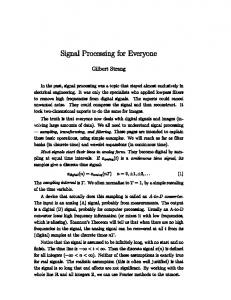
A vision system depends intimately on its input, and it is noteworthy that in so wellestablished a field as photography, three important technologies have recently come into prominence. Depicted in Figure 1.1, these are the time of flight camera, which employs the finite propagation rate of light to measure depth; the structured light camera, which employs known projected patterns of light to estimate depth; and the plenoptic (also light field) camera, which employs multiple-aperture optics to implicitly encode texture and depth. This work is concerned with exploring the third of these, plenoptic cameras, as a means of simultaneously enabling greater robustness and simplicity in computer vision. The key 1

2

1.1 Motivation

(a)

(b)

(c)

Figure 1.1 – Three camera technologies enjoying recent prominence: (a) time of flight, (b) structured light, and (c) plenoptic.

motivations for this lie in field robotics, including the challenging environments, limited platforms, and an opportunity to closely couple optics and computing in a powerful integrated sensor.

1.1.1

Robustness in Computer Vision

Working solutions have been demonstrated across a range of domains for many of the major problems in computer vision, including mapping, modelling, localization, tracking, classification and recognition [8, 38, 92, 118, 154, 155, 201]. The unveiling of Google’s driverless car in 2011, and subsequent issuing of a license for it to operate on Nevada’s streets in 2012, are testament to the strength of modern computer vision technologies, amongst others. However, because they operate outside, field robots – including the Google driverless car – are sometimes exposed to visually challenging conditions capable of impeding their vision systems1 . Dust, rain, fog, snow, smoke, glare and low light are all regularly encountered by unmanned ground vehicles (UGVs), unmanned aerial vehicles (UAVs) and marine unmanned surface vehicles (USVs). Autonomous underwater vehicles (AUVs) must contend with the underwater equivalents, including murky water, suspended particulate matter and dynamic light effects such as the light beams and caustics depicted in Figure 1.2. These conditions can interfere with even the most sophisticated vision algorithms, including those that have evolved over millions of years. Anyone who has driven in drifting snow, depicted in Figure 1.2(b), knows that this simple scenario can cause the convincing illusion that the 1

In this work we define field robotics broadly as the application of robotics technologies in outdoor settings, especially in unstructured, natural environments.

3

1.1 Motivation

(a)

(b)

(c)

Figure 1.2 – Examples of challenging environmental conditions: (a) Fog seriously impacts contrast in this aerial photo; (b) drifting snow can fool even the human visual system; and (c) dynamic caustics and light beams dominate the visual information in this underwater scene.

1.1 Motivation

4

snow is static, and that the road is drifting – an unnerving sensation when one’s goal is to stay on the road! Even in ideal conditions, the complex, unstructured environments in which field robots operate can complicate vision. Straight edges and right-angled corners are generally absent, and outdoor scenes often display a high degree of self-similarity – one small patch of coral, coastline or grassy plain looks very much like hundreds of other small patches, often at multiple scales. These features can interfere with computer vision algorithms developed for more regularly structured environments. Finally, the mobile nature of the robotic platform is responsible for a further class of hindrance. Field robots are not generally static, indeed they are sometimes incapable of remaining still due to competing forces such as wind and water currents, or a need to maintain lift or steering authority. This motion combined with complex scene structure results in nonuniform projected motion which complicates some tasks. Change detection, for example, can be accomplished by simple pixel differencing, but only if the camera is static or the scene planar. Platform motion also limits exposure times due to motion blur, and complex 3D scene structure can necessitate a wide depth of field, limiting maximum aperture diameter – both of these result in lower light sensitivity and reduced image quality in low-contrast scenarios. We take these challenges as motivation to develop robust computer vision algorithms suitable for use in challenging field conditions – one would certainly want Google’s driverless car to be as capable as possible in conditions as common as rain, fog, or snow. In addition to improving performance in existing applications, we are motivated by the possibility of broadening the range of conditions under which robotic deployments are possible.

1.1.2

Computational and Behavioural Simplicity

We have identified an opportunity to improve the robustness of computer vision in field robotics. However, with the rich information accessible through other sensors one might ask why vision should be considered at all. Historically, roboticists have found great success in addressing challenging conditions by turning to alternative sensing modalities. Lidar sensors, for example, robustly generate 3D point cloud models using active, laser-based sensing. They have been employed in mobile robotics since as early as 1977 [103], and directly

1.1 Motivation

5

Figure 1.3 – Cameras offer more information at lower weight, size and monetary costs than any other sensor; modern cellular telephones perform face detection and image registration as enabled by these economical sensors.

provide detailed and accurate 3D scene models with minimal external computation. Other sensors employed in robotics include inertial navigation systems, global positioning system (GPS) receivers, compass, Doppler-based odometry, radar, acoustic imaging, infrared and acoustic range-finding, and pressure-based altimeters and depth sensors. Increasingly, two of the alternative camera technologies depicted in Figure 1.1, the time of flight and structured light-based RGB-D sensors, are also finding adoption within the robotics community [132, 148, 189]. We observe that in the diverse range of available sensors, cameras occupy a unique niche by measuring dense colour and textural detail that are not accessible by other means. Furthermore, cameras present no possibility of inter-sensor interference, unlike many active sensors, and are appropriate for outdoor use, unlike active infrared sensors such as Microsoft’s structured light-based Kinect. We further note that cameras deliver more information at a lower cost than other sensors. At the time of writing, one particular off-the-shelf camera – depicted in Figure 1.3 – costs less than USD✩4, delivers 300,000 pixels 30 times a second, draws 120 mW of power, and fits inside a cube 3.2 mm on a side, including optics. A similar 8 Megapixel model comes at a modest increase in size and cost. Even including the cost of computing hardware, this is orders of magnitude less expensive than lidar or imaging sonar, in terms of financial cost, size, weight and power consumption. Indeed, applications such as face tracking and image mosaicing are already in common use on power-limited, low-cost and compact mobile platforms – we refer of course to cellular telephones – and this is only possible by virtue of lightweight visual sensing. We hypothesize that an important barrier to the widespread adoption of visual sensing is the complexity of vision algorithms. In this respect, tightly integrating cameras and computing

1.2 Problem Statement

6

as in the mobile phone example above makes good sense. Indeed we attribute much of the success of RGB-D sensors to their pre-packaging of the transmission, sensing and computing required to directly deliver co-registered depth and colour images. Similar attempts with passive cameras, however, have not yet enjoyed the same level of success. This is at least partially a symptom of the complexity of existing vision algorithms, both in terms of computational burden and range of behaviour. As an example, depth estimation from stereo matching shows a much more complex range of behaviours and failure modes than RGB-D cameras, making the latter significantly easier to integrate into robotics applications. These observations underline an opportunity to develop simple and consistent computer vision algorithms, enabling the development of tightly integrated and easily deployed sensors. Aside from filling an important general-purpose niche, we expect that the modest size and power requirements of such devices would enable new levels of autonomy in small robotic platforms. This is especially true where external sensing is presently required, as in the motion capture arenas employed in much of the recent quadcopter research.

1.2

Problem Statement

Based on the discussion above, there exists a clear opportunity to advance computer vision in field robotics in two important areas: 1. Increasing robustness to difficult environmental conditions, in unstructured scenes and under the constraints of a moving platform; and 2. Simplifying algorithms, both in terms of computational burden and behaviour, to enable tightly integrated, predictable and easily deployed vision systems. We expect that progress under these broad objectives will yield improved performance in existing applications, while allowing new forms of autonomy where previously prohibited by environmental conditions or limited sensor payloads. To address them, we turn to the third technology depicted in Figure 1.1, the plenoptic camera. These passive devices share many of the advantages of conventional cameras, but measure a rich, 4D light field structure that implicitly encodes both geometry and texture. Our hypothesis is that plenoptic cameras can enable the algorithms required to accomplish the goals enumerated above. The key challenges in showing this to be true involve understanding the properties of plenoptic signals and developing the algorithms required to exploit them.

1.3 Contributions

1.3

7

Contributions

The broad topics addressed by this thesis are: 1. Calibration and rectification of plenoptic imagery; 2. Improved image quality in low-contrast scenarios; 3. Mitigation of environmental factors such as snow, rain and particulate matter; and 4. Dramatic simplification of a set of nontrivial problems in computer vision. The specific contributions are: Calibration and rectification – partially published as [45] • A novel pinhole/thin lens model which better describes the real-world behaviour of lenslet-based plenoptic cameras than previous models; • A novel 4D plenoptic intrinsic matrix based on the physical camera model, which linearly and reversibly relates rectified pixels and rays; • The first published calibration scheme appropriate to lenslet-based cameras including a novel ray reprojection calibration objective function; and • Practical decoding and rectification methods appropriate to lenslet-based cameras. Contrast enhancement and interference mitigation – partially published as [46] • Identification of the frequency-domain region of support of the light field as the hyperfan at the intersection of a 4D hypercone and a 2D fan – this is more detailed and selective than previous descriptions; • Development of novel, inseparable 4D hyperfan filters surrounding this shape; and • A demonstration that these effect volumetric focus, contrast enhancement in low light and murky water, and attenuation of interference including occluding particulate matter. Visual odometry – partially published as [48] • A novel geometric derivation yielding methods for featureless 6-degree-of-freedom (DOF) visual odometry, culminating in a closed-form plenoptic flow solution; • Improvement of previously-published closed-form gradient-based depth estimation; • A novel, additive rendering method which generates novel views based on plenoptic motion decomposition; and • A novel adaptation of plenoptic flow to lenslet-based imagery.

1.4 Outline

8

Distractor isolation – partially published as [49] • Closed-form identification of dynamic scene elements in the presence of nonuniform apparent scene motion, through a novel method employing the residuals of plenoptic flow; and • Linear distractor isolation and removal from spatially co-linear and temporally disjointed monocular image sequences, through novel spatio-temporal light field construction and filtering. Parts of this work also appear in [112, 143, 152].

1.4

Outline

Several plenoptic devices are described throughout the literature, and Chapter 2 lists some of the diversity of names under which these and light field processing concepts appear. It also provides background relevant to the remainder of the thesis, including a description of the theory of operation of a few important light field camera models. Their compact nature makes lenslet-based plenoptic cameras particularly suitable for field robotics. Chapter 3 lays the groundwork for employing these cameras by developing appropriate decoding, calibration and rectification schemes. A physically based 4D plenoptic intrinsic matrix is derived which straightforwardly and reversibly relates pixels and rays, and a practical calibration objective function is presented. The proposed pinhole and thinlens camera model underlying this chapter is shown to more accurately represent the physics of lenslet-based cameras than previous models. In Chapter 4 the frequency-domain shape of plenoptic signals is derived as the hyperfan at the intersection of a 4D hypercone and a 2D fan. Though past work has examined the frequency content of light fields, this treatment differs in its level of precision, identifying the highly-selective hypercone and hyperfan shapes, and proposing the irreducibly 4D filters required to fully exploit them. The proposed hyperfan filters are shown to focus on a volume, rather than a plane, effectively maintaining depth of field. They are also shown to dramatically improve contrast in low light and through attenuating media such as murky water and fog, while reducing the impact of noise and occluders such as snow, rain and underwater particulate matter. Quantitative results demonstrate significant improvement over previous work.

1.4 Outline

9

In Chapter 5, the classically nonlinear problem of visual odometry is reduced to a closedform system of linear equations. A geometric derivation yields a series of methods for performing featureless 6-DOF visual odometry, culminating in plenoptic flow, a closed-form generalization of optical flow which directly estimates camera motion from first-order derivatives. Although prior work has demonstrated similar equations, the geometric derivation presented here provides unique insights allowing an improved method of closed-form depth estimation, and an additive method for rendering novel views based on plenoptic motion decomposition. A method is also derived for applying plenoptic flow to lenslet-based imagery, and an extension of plenoptic flow to distractor isolation is presented in the following chapter. In Chapter 6 the isolation of dynamic elements from a static background is considered, a task complicated by nonuniform apparent motion associated with a mobile camera. An elegant closed-form solution to this conventionally complex problem is presented which, through an adaptation of plenoptic flow, identifies dynamic objects as those breaking the rules of parallax motion. A second solution demonstrates an application of light field principles to conventional imagery, co-registering spatially co-linear but temporally disjointed monocular images into a plenoptic signal. This allows distractor isolation and removal using a linear filter and its inverse. Finally, Chapter 7 draws conclusions and indicates directions for future work. Throughout this work, non-iterative (i.e. direct) closed-form and linear methods are emphasized. These have predictable behaviours and constant runtimes, addressing the goal of simplicity set out above. They are also noise-tolerant and, in the case of the hyperfan filter, noise- and interference-attenuating, addressing the goal of robustness. The non-iterative and closed-form nature of the methods presented here make them particularly suitable for hardware implementation. By employing field programmable gate arrays (FPGAs) or application-specific integrated circuits (ASICs), very compact, responsive, high-throughput and power-efficient implementations are possible. This line of research is beyond the scope of the present work, but the curious reader is referred to [113–115, 196].

Chapter 2

Background “Nonsense is that which does not fit into the prearranged patterns which we have superimposed on reality... Nonsense is nonsense only when we have not yet found that point of view from which it makes sense.”

2.1

– Gary Zukav

Related Work

We have identified field robotics as our primary motivation, and will be taking on specific computer vision problems relevant to the field. We employ a specific sensor occupying a niche within the spectrum of camera technologies, and we focus on a family of lightweight, linear and analytic filtering and estimation approaches deriving from the principles of information theory and signal processing. Clearly, this work lies at the intersection of many disciplines. Of the related work, plenoptic signal processing is undoubtedly the most directly relevant – Section 4.2 outlines a partial history of the field. The work presented here originates chiefly from the confluence of multi-dimensional signal processing (MDSP) and image-based rendering. The latter of these is the context in which the first plenoptic modelling and light field papers came about [69, 102, 120]. Its underlying principle is to simplify the rendering of computer graphics by changing the emphasis of the model: Rather than capture the geometry and texture of a scene, image-based rendering models the behaviour of the light permeating it. This data-driven approach allows very fast rendering from arbitrary 10

2.2 A Rose by Any Other Name

11

viewpoints, and from arbitrary cameras, allowing changes in focus, for example – this is a key feature of consumer-driven plenoptic cameras today. The light field models at the core of image-based rendering are directly observable by plenoptic cameras, and rendering from light fields is an active area of research which continues to inform tasks in plenoptic analysis [15, 65, 67, 108, 110]. The other key field driving this work is MDSP, which examines the underlying properties of signals in order to develop efficient, often linear and analytic solutions to complex problems. The 3D plane wave analysis originating in MDSP and having applications spanning astronomy, acoustics, radio and video processing [20, 81, 112] has strong parallels to the 4D planar analysis applicable to light fields. Indeed, a generalization of plane wave filtering to 4D allows depth selective filtering in light fields [43]. MDSP underlies much of robotics and computer vision. For example some of the recent, high-profile work on pulse detection from video sequences is essentially a rediscovery of concepts from MDSP, employing spatiotemporal bandpass filters to simply and robustly detect small, periodic signals [12, 198]. The specific technical questions tackled in this thesis are calibration, filtering, odometry and change detection, each of which have rich bodies of research dedicated to them. Rather than review these here, each chapter provides its own literature review. Modern plenoptic signal processing addresses many more problems than these, of course, with recent work spanning a broad range of topics including labelling [184], video stabilization [164], gas flow reconstruction [84], depth estimation [16], and compressive sensing-based acquisition and compression [119].

2.2

A Rose by Any Other Name

The technology enabling the present work is the plenoptic camera, which in the introductory chapter we noted has only recently come into prominence. Indeed, off-the-shelf cameras have only become commercially available in the last few years. Anecdotally, exposure of plenoptic processing ideas is steadily increasing, and interestingly seems to be inversely proportional to level of integration: Exposure is highest in imaging, lower in computer vision, and lowest in robotics. The technology behind plenoptic cameras is not new, however, and the key ideas behind it have appeared in different domains and under different names for more than a century.

2.2 A Rose by Any Other Name

12

The history of plenoptic photography has appeared elsewhere [64], and so rather than reproduce it here this section seeks to expose the many names and keywords under which similar ideas have been explored. We do this with the hope of reducing duplication of effort due to a complex taxonomy of nomenclature that can easily conceal relevant research. A list of keywords is included at the end of the section for convenience. Throughout this thesis the terms “plenoptic camera” and “light field camera” are used essentially interchangeably. Historically, plenoptic was reserved strictly for the 7D function describing all light passing through all space over all time, as described by Adelson and Bergen in 1991 [2]. The modern interchangeability is due largely to Lytro’s popularization of their commercial device under the name plenoptic camera, though we do note earlier usage, including Adelson’s 2002 paper describing depth estimation from a plenoptic camera [1]. The term light field was itself borrowed from Gershun’s 1936 work, in which it refers to a different concept, the irradiance vector as a function of position [66]. Levoy and Hanrahan were the ones to borrow this term, in their 1996 paper on image-based rendering [102] – they do acknowledge the discrepancy between theirs and the earlier usage, further noting that some physicists later turned to the term photic field to more clearly distinguish the concepts [124], though that term is not in common usage. In the same year that Levoy and Hanrahan published their light field work, Gortler et al. published a similar image-based rendering paper under the name lumigraph [69]. Astronomers employ wavefront sensors to control adaptive optics. These first appeared as an aperture array device developed by Hartmann in 1900 as a means of tracing the light passing through a telescope [74]. Though its use is specific to astronomy, to the author’s knowledge this is the earliest example of a light field sensor. In their 1971 work, Shack and Platt describe a refinement on Hartmann’s array employing lenslets [159], and this is the variant in common use today under the name Shack-Hartmann sensor. Outside astronomy, Lippmann created the first plenoptic sensor under the name integral photography in 1908 [105]. The term polydioptric camera was introduced by Neumann et al. [129] to elicit the multiple refractive paths associated with physical plenoptic camera embodiments. Neumann argues for use of this term to clearly distinguish between the continuous-domain plenoptic function and the discrete subset that can be measured by practical devices.

13

2.3 Plenoptics

The term compound eye [173] is sometimes employed for lenslet and array-based cameras, and cameras employing attenuating masks appear under the names mask-based capture, dappled photography and coded aperture imaging [10, 96, 100, 179, 199]. Early, primarily 2D analyses of light fields employed the name epipolar image or epipolarplane image [11, 18], and these terms still occasionally appear. A camera array [190] captures a light field, as does an appropriately configured camera gantry [43]. Work sometimes appears under variants of the array idea, including catadioptric array [172, 204], reflective array, refractive array, and multi-axial imaging [4]. A less well-structured collection of viewpoints is not conventionally referred to as a light field camera, but ideas applicable to plenoptic imaging sometimes appear in the context of multiple camera or multi-view scenarios [165, 205]. Finally, light field cameras belong to the greater classes of generalized and computational cameras [58, 97, 187]. Table 2.1 – Keywords under which plenoptic processing concepts appear

aperture array camera array camera gantry catadioptric array coded aperture imaging compound eye computational camera computational photography dappled photography epipolar image epipolar-plane image generalized camera integral photography

2.3

light field lumigraph mask-based camera multi-axial imaging multiple camera multi-view photic field plenoptic camera polydioptric camera reflective array refractive array Shack-Hartmann sensor wavefront sensor

Plenoptics

It is important to understand that light is a higher-dimensional phenomenon than one might intuitively conclude. A 2D photo, after all, goes most of the way towards representing what we see with our own eyes, minus depth. So, goes the reasoning, perhaps light is a 3D phe-

14

2.3 Plenoptics

nomenon? In 1991, Adelson and Bergen proposed that light could be understood in a much higher-dimensional space [2]. Their “plenoptic function” – so-named by prepending optics with plenum, a Latin word meaning “full” – describes light in seven dimensions: time (1), space (3), direction (2) and frequency (1). One might also add mode of propagation, in particular polarization, to this list. The plenoptic function inspires us to contemplate light not in terms of objects, geometry and texture, but rather in terms of light rays themselves. A scene is no longer a set of surfaces, but rather a volume through which light rays flow, and the act of seeing is no longer one of reaching out to objects with rays, but of measuring the light passing through two openings, the pupils of our eyes. This shift to thinking about the light itself is what allowed Levoy and Hanrahan’s imagebased rendering [102].

Because the plenoptic function represents all the light moving

through a scene, determining what a specific camera, at a specific point in space would see is a simple matter of querying the plenoptic function with the appropriately selected rays – those that pass into the camera. For a suitably sampled representation of the plenoptic function, this querying requires only interpolation.

2.3.1

The Light Field

The plenoptic function is of a higher dimensionality than is required for image-based rendering, and a key insight in [102] was to reduce the dimensionality to a 4D subset, the light field, making the storage requirements associated with representing the plenoptic function significantly more manageable. Similar parameterizations had previously been explored in optics [72, 197], but this was the first time such a parameterization was employed for processing digital images. Time was discarded in favour of static scenes, and frequency replaced with the three colour channels typical of digital colour representation. Note that we exclude the three colour channels when counting the dimensionality of the light field, as they are generally treated independently, akin to having three 4D signals. The astute reader will have noticed that an extra dimension remains unaccounted for in the above: Three spatial and two directional dimensions add up to five, not four. An important insight brought to light in [102] allows removal of one of the spatial dimensions: Light rays do not change in value along their direction of propagation – at least, not until they hit

2.3 Plenoptics

15

Figure 2.1 – Two-plane parameterizations of light rays – shown is the relative two-plane parameterization. The points of intersection of a ray with two parallel planes completely describes its position and orientation in space. By convention, the s, t plane is closer to the camera, and the u, v plane is closer to the scene.

something, or pass through an attenuating medium. This realization allows light rays to be parameterized in terms of four dimensions instead of five. A common way of doing so measures each ray’s points of intersection with two parallel reference planes, requiring only four numbers to describe the ray, two for each of position and direction. The caveats in the above argument – that the light rays not impact a surface or pass through attenuating media – are not as restrictive as they may first appear. Of course all the light rays we might be interested in eventually do one or both of these things, but in the unobstructed space of a scene through which the camera passes they do not. This means, for example, that a light field model of a closed door will allow rendering of novel views in front of the door, but not behind it.

2.3.2

Light Field Parameterizations

Throughout this work we employ light field parameterizations in which light rays are described by their points of intersection with two parallel planes: an s, t plane, by convention closest to the camera, and a u, v plane at distance D, by convention closer to the scene. The continuous-domain light field signal L(s, t, u, v) describes all light rays passing through

2.3 Plenoptics

16

the s, t and u, v planes. The relative two-plane parameterization, depicted in Figure 2.1, is so-called because the ray’s intersection with the u, v plane is expressed relative to its intersection with the s, t plane, as shown. In the absolute two-plane parameterization, U and V are expressed as s and t, in absolute coordinates. Though we employ uppercase U, V to distinguish absolute coordinates, lowercase u, v can refer generically to both variants. It is often most convenient to align the global coordinate system with the two-plane parameterization, as shown in Figure 2.1, so that s and x are aligned, and likewise for t and y. The following section describes a camera array as a simple form of light field camera, and it is most convenient to place the apertures of such an array within and aligned with the s, t plane – such a set of cameras and their apertures are depicted in the figure as cubes and circles in the s, t plane. One of the advantages of the relative two-plane parameterization is that, if one selects D to equal the focal length of the cameras in the array, u and v then coincide with physical coordinates on the image sensor. One can think of the s, t plane as selecting a camera, and u, v as selecting a pixel. The two-plane parameterization describes rays in terms of position and direction, and so the terms angular and spatial are sometimes employed to describe these dimensions. One interpretation is that s and t fix the position of a ray, while u and v fix its direction. In this interpretation, s and t are spatial, and u and v are angular dimensions – this convention is followed throughout the thesis. There are other interpretations, however, and we could think instead of u, v fixing ray position – especially in the absolute parameterization – and s, t fixing direction. Sometimes the scene is the focus of a discussion, and one might discuss spatial and angular resolution of light rays leaving surfaces within the scene. Again, we employ the first of these three interpretations. Alternatives to the two-plane parameterization exist, most notably the spherical-Cartesian parameterization, also known as the one-plane parameterization. This parameterization describes a ray’s position using its point of intersection with a plane, and its direction using two angles, for a total of four parameters. Unlike the two-plane parameterization, which cannot describe rays that run parallel to the reference planes, the spherical-Cartesian system can describe rays passing in all directions. Note that these parameterizations represent essentially the same form of information, the 4D light field, and conversion between them is possible except where rays run parallel to the reference planes.

2.3 Plenoptics

2.3.3

17

The Camera Array

A major strength of the light field representation is that the light field of a scene can be directly measured by a passive optical system. This is in contrast to scene geometry, which can only be measured by interacting with the scene via active methods like lasers, sonar, or contact sensors. A variety of methods exist for measuring light fields, and some of these were listed in Section 2.2. Of the light field measuring devices, an array of monocular cameras is in many ways the most easily understood [190]. The array of images measured by such a device straightforwardly maps to a 4D light field, with camera position determining s, t, and pixel position determining u, v, as depicted in Figure 2.1. Many of the properties of light fields are also most easily understood in terms of camera arrays. For example, the increased light gathering of a light field camera is easy to see: In the case of an N × N grid of cameras, the amount of light captured is straightforwardly N 2 the light captured by a single camera having the same depth of field.

2.3.4

The Lenslet-Based Camera

A second type of camera employs an array of lenslets within the optical path of a monocular camera [135]. Depicted in Figure 2.2, the principle is to split light across different pixels based on its direction of arrival. The main lens focuses the scene on the lenslet array, and the lenslet array focuses the pixels at infinity, or equivalently on the main lens. That this measures a light field is less intuitive than in the case of a camera array. However, the idealized model shown in Figure 2.3 shows how tracing a ray for each pixel through the camera and into the scene reveals a virtual aperture array in front of the main lens. For a camera with N × N pixels beneath each lenslet, there are N × N such virtual cameras. This model is elaborated in Chapter 3. While it is evident that an array of cameras gathers more light than a single camera, it is less obvious that a lenslet-based camera also does so. This well-established fact has appeared in the literature [14, 135], but is often misunderstood or overlooked. It is our hope that an informal but intuitive explanation will assist in clarifying this important point. When we compared a single camera and an array, we did so without changing depth of field. This is important because depth of field and light gathering trade off directly. When we

2.3 Plenoptics

18

Figure 2.2 – The lenslet-based plenoptic camera – Light from an object in the scene (right) passes through the main lens (blue), and is focused on a lenslet array (green). The lenslets split the incoming light across many pixels (left), based on direction of arrival. A single pixel is highlighted in yellow, illustrating the aperture size of a conventional camera with the same depth of field.

say a camera gathers more light, we could equivalently say it has a wider depth of field – the key is the ratio between the two. The depth of field of a camera is determined by the spatial extent of the rays integrated by each pixel. Referring to Figure 2.2, the yellow cone of light represents the rays integrated by one pixel, and the cone’s extents at the aperture determine depth of field. This is akin to the baseline of a stereo camera: Smaller changes in depth are observable with larger baselines, and so it is with the pixels of a camera. Pixels with smaller “baselines” – extents at the aperture – are less sensitive to changes in depth, and therefore have a wider depth of field. In a conventional camera pixels integrate light across the whole aperture, and so the “baseline” of every pixel equals the full aperture diameter. This can be seen by replacing the lenslet array in Figure 2.2 with a pixel array, one pixel per lenslet, to yield a traditional camera. It should be clear that the path highlighted in red depicts the light integrated by a single conventional pixel, and that it has a full-aperture baseline. In the plenoptic camera, lenslets split arriving light across multiple pixels, and so a single pixel integrates across a fraction of the aperture, as depicted by the yellow path. The smaller baseline of this pixel yields a wider depth of field. So, to make a conventional camera with the same depth of field as the plenoptic camera depicted in Figure 2.2, it would need to narrow its aperture to match the yellow path.

19

N=4

2.3 Plenoptics

i,j k,l

i,j k,l

s,t

U,V

Figure 2.3 – An idealized model shows how the lenslet array results in a virtual camera array in front of the main lens. Here a single ray has been traced starting from each pixel on the left at the i, j plane, passing through the nearest lenslet at k, l, then the main lens at s, t, and finally into the scene where the u, v reference plane has been placed to coincide with the array of virtual cameras. Ray colour illustrates the N virtual cameras, and the inset depicts the N = 4 pixels per lenslet in this example.

Stated the other way around, if we were to start with a conventional camera with an aperture matching the yellow path, we could construct a plenoptic camera with the same depth of field but having the much wider aperture depicted by the red path. In the case of camera arrays with N × N cameras, we concluded there would be a gain in light gathering of N 2 . Strikingly, for a lenslet-based camera with N × N pixels beneath each lenslet, the aperture diameter can be increased by a factor of N , again resulting in an N 2 increase in light gathering. Referring to Figure 2.3, we see that this lines up with our simplified model, which predicts an equivalent N × N virtual camera array.

2.3.5

Focused Lenslet-Based Cameras

In 2009 Lumsdaine and Georgiev proposed a modification of the lenslet-based plenoptic camera [109]. In the originally proposed camera, the main lens focuses on the lenslets, as shown in Figure 2.2. In the “focused” plenoptic camera, sometimes called “plenoptic camera 2.0”, the main lens is focused elsewhere, either in front of or behind the lenslets, and the lenslets are focused to match. This increases the degrees of freedom in designing the camera, allowing different tradeoffs between angular and spatial resolutions, and offering different focusing behaviour than available with the traditional lenslet-based camera. A

2.3 Plenoptics

20

further variant on the focused plenoptic camera is the “multi-focus” plenoptic camera which employs interleaved lenslets of different focal lengths to extend depth of field [60]. Although we do not specifically address the focused plenoptic camera, much of our development is concerned with the structure of the 4D light field, which is independent of the camera technology used to measure it. This is because it is possible to resample light fields with different parameterizations into the two-plane parameterizations that we employ here. A practical example is presented by Wanner et al. [182], in which images from a focused plenoptic camera are converted to an epipolar form suitable for the two-plane parameterization. This is possible because all 4D plenoptic cameras measure fundamentally the same kind of information, the light field. The optical properties of these cameras do differ, however, and for a generalization of the depth of field discussion above to the focused plenoptic camera, the reader is referred to [63].

2.3.6

Tradeoffs

Of the camera technologies discussed here, the compactness of lenslet-based cameras makes them particularly appealing in robotics applications – certainly more so than traditional, large camera arrays. As we shall see in Chapter 3, manufacturing processes for both the pixels and lenslets going into lenslet-based cameras are very precise, reducing the modes of imperfection to a few degrees of freedom. Conventional camera arrays, on the other hand, are difficult to align, and require many more degrees of freedom to describe their imperfections, especially in inter-aperture pose variations. The characteristics of forthcoming miniaturized camera arrays like the one depicted in Figure 1.1(c) are yet to be seen, though their separate lenses may behave much like camera arrays. An important characteristic of lenslet-based devices is that they trade off angular and spatial resolutions [62, 141]. For a 9 Megapixel sensor and 10 × 10 pixels per lenslet, the resulting light field has 10 × 10 samples in s and t, and 300 × 300 pixels in u and v. A conventional camera employing the same sensor would measure one sample in s and t, and 3000 pixels in each of u and v. A common interpretation is therefore that the plenoptic camera has a fraction of the resolution. This could be restated as one form of information – angular samples – being traded for another – spatial samples.

2.3 Plenoptics

21

Viewing this as a tradeoff of course assumes that pixel count is somehow fixed. However, the number of pixels employed in a given robotics application often has more to do with external considerations – bandwidth, memory, optics and minimum resolution requirements – than by our ability to construct high-pixel-count sensors. 50 Megapixel sensors are a modern reality, though few robotics applications would take on such a device as they simply have no call for that many pixels. If we take the view that pixels are in abundant supply, the question becomes how to best employ them. If one were to expend as many pixels as were available – say 50 Megapixels – on angular samples, or trade some off for spatial samples, which scenario would yield the most information about the scene? Which would yield the most useful information about the scene for a given task? It is our suspicion that most applications would benefit from a balance of both forms of information. Importantly, the idea that plenoptic cameras reduce resolution is only accurate if one assumes a fixed pixel count. As a concrete example, Chatterjee and Milanfar in their 2010 paper “Is Denoising Dead?” and follow-on work [26, 27] examine theoretical limits on the extent to which denoising techniques can improve image quality. They later use this to derive a near-optimal patch-based denoising method [28]. The method we describe in Chapter 4 can significantly outperform even this nearly optimal method, but only because it benefits from the extra information gathered by the plenoptic camera. The comparison is fundamentally unfair, but it does highlight that if the end-goal is performance in contrast-limited environments, plenoptic sensing offers a significant advantage. A related tradeoff in plenoptic imaging is that of bandwidth. For most applications plenoptic imaging yields higher data rates than conventional imaging. This is a consequence of the fact that these cameras capture more information, and it has drawbacks in terms of computation, transmission and storage requirements. In the introduction we highlighted these concerns, proposing that tightly coupling computation and sensing might help address them. An integrated sensor could directly deliver processed, low-bandwidth information that benefits from the added information of plenoptic sensing, but shields the system from the associated increase in bandwidth. Table 2.2 explores design tradeoffs in a set of representative conventional and lenslet-based plenoptic cameras. All these cameras feature a field of view (FOV) of 52 degrees and are focused on a plane 2 m in front of the camera. The resolution column “Res.” shows

22

2.3 Plenoptics Table 2.2 – Exploring tradeoffs in camera design Model

Focal length (mm)

Pixel pitch (µm)

Conventional Cameras DOF 7 7 Light 7 7 Lenslet-Based Dense Large, DOF Large, Light Same, DOF Same, Light

Pixels

Res. (mm)

Near focal (m)

Far focal (m)

F/#

DM (mm)

Relative DOF light

1M 1M

2 2

0.609 1.27

∞ 4.67

8 2

0.875 3.5

1 16

Wide Narrow

2 2 2 8 8

0.609 0.609 1.27 0.197 0.609

∞ ∞ 4.67 ∞ ∞

2 8 2 2 0.5

3.5 3.5 14 3.5 14

16 16 256 16 256

Wide Wide Narrow V. Wide Wide

Plenoptic Cameras, N = 4 × 4 7 1.75 16M 28 7 16M 28 7 16M 7 7 1M 7 7 1M

the pixel footprint on the focal plane, while the near and far focal distances are those for which the circle of confusion on the sensor is equal to the pixel pitch, beyond which objects experience defocus blur. “F/#” is the F-number of the camera, and DM is the diameter of the camera’s aperture. The “Relative light” column reflects the total light gathered by the camera, expressed relative to the light gathered by the first camera in the table. The final “DOF” column is a qualitative description of depth of field, as determined by the near and far focal distances, and is included to facilitate comparison. The first two rows in Table 2.2 depict conventional cameras prioritizing depth of field and light gathering, respectively. These two features trade off directly, and so a wide depth of field and enhanced light gathering are not simultaneously possible. The next five cameras depict a variety of plenoptic cameras with N = 4 × 4 pixels per lenslet. The first of these lenslet-based cameras employs a denser sensor than the equivalent conventional cameras, and its performance simultaneously offers a wide depth of field and enhanced light gathering, while keeping all other features, e.g. resolution and field of view, fixed. The light gathering of this camera is proportional to N 2 which, in this case, is 4 × 4 = 16. Rather than employing a denser sensor, the next two plenoptic cameras in Table 2.2 employ larger sensors to obtain more pixels, necessitating a change in focal length to obtain the same field of view. These cameras prioritize depth of field and light gathering, respectively, and the performance of the first matches that of the dense sensor example, while the second opens its aperture to gather still more light – proportional to N 4 = 256 times the light – at the cost of a narrower depth of field. The final two cameras employ the same sensor as the conventional cameras and therefore show a reduced resolution. However, larger pixels gather more light and are less sensitive

2.3 Plenoptics

23

to defocus blur, and so the first of these cameras offers a very wide depth of field, while the second offers significantly enhanced light gathering. We note that the final camera in the table is probably not physically realizable due to its requirement for an F/0.5 lens, but it does illustrate a useful point, that depth of field and light gathering trade off in lensletbased plenoptic cameras, but for a significantly more favourable ratio than in a conventional camera. The most important observation from this Table 2.2 is that lenslet-based cameras always gather more light for a given depth of field than conventional cameras, on the order of N 2 times the light for the fairest comparison, and as much as N 4 times the light if a resolution reduction is allowed. Though the above analysis ignored effects such as diffraction, aberrations, and attenuation introduced by the lenslet array, gains as significant as N 2 or N 4 will generally dominate over these higher-order effects.

2.3.7

Light Field Visualizations

We will be examining the characteristics of 4D plenoptic signals, and as such some means of visualizing these signals will be useful. In general we will be slicing the light field into 2D images. A u, v slice of the light field fixes s and t and examines the signal as it varies in u and v. Returning to the two-plane parameterization and camera array analogy depicted in Figure 2.1, it is clear that this corresponds to examining what a single camera in the array sees. An example of a u, v slice is depicted in Figure 2.4. It is often useful to examine different pairings of dimensions from the light field, in particular s, u and t, v. Examples of these slices are also shown in Figure 2.4. The s, u slice is taken for the v value highlighted by the red line, and the t, v slice is taken for the u value highlighted by the blue line. It is also possible to visualize the 4D light field as an array of slices. This is akin to tiling all the images captured by the cameras in an array. Figure 2.5 shows an array of u, v slices arranged according to their s, t positions. Notice the compact convention we follow in labelling these axes. Here s and t are the outer dimensions, while u and v are the dimensions of the individual tiles, but different permutations of dimensions are employed throughout the thesis.

2.3 Plenoptics

24

Figure 2.4 – Visualizing subsets of the 4D light field in 2D slices. The large u, v slice can be thought of as a conventional image taken from a camera sitting on the s, t plane. The s, u and t, v slices – sometimes referred to as epipolar images – show characteristic straight lines with slopes which, as discussed in Chapter 4, reflect depth in the scene.

2.3 Plenoptics

25

Figure 2.5 – Visualizing the light field as an array of u, v slices arranged in s, t. Here each tile is a u, v slice like the one shown in Figure 2.4, and behaves like a conventional image taken from a camera sitting at a specific location on the s, t plane. Tiles are arranged by their s, t positions. Note the compact axis labelling convention which is followed throughout this work.

2.4 Conventions

2.4

26

Conventions A new Mars lander is en route to the red planet when suddenly all contact is lost. The project manager, lead scientist, and lead engineer are called in to diagnose the situation, and they quickly discover the vessel has collided with a previously unknown Martian moon. The manager is furious, “Why didn’t we know about this?!” The scientist is elated, “We’ve discovered a new moon!” But the engineer barely reacts. “Don’t worry about that,” he says, “it’s just noise.”

2.4.1

Noise and Interference

Noise and interference are often bundled into a single concept in informal conversation. We will take a cue from telecommunications, the birthplace of the information theory that drives much of computer vision, and instead adopt a strict distinction between the two [147, 160]. The absurdity of referring to a celestial body as “noise” in the above joke helps underline the difference between these concepts: Noise is random and unpredictable, arising in any receiver of electromagnetic waves, including cameras, due to the physical characteristics of the measurement instrument. It has less to do with the incoming signal, and more to do with what the receiver does to that signal. Interference, on the other hand, is the presence of competing, real, physical entities within the signal before it is even received. Competing users in a radio communication system and occluders between the camera and the scene in photography are good examples of interference. That we identified noise as being both random and unpredictable may appear redundant, but it helps distinguish it from other random but predictable phenomena. The random pattern of gain fluctuations across the pixels of a camera – a phenomenon commonly and confusingly referred to as “fixed-pattern noise” – is an example of a random but predictable (fixed) phenomenon. Having measured the fixed pattern noise for a sensor, it can be compensated for, at which point it is neither noise nor interference, but part of our model of how the camera behaves.

2.4 Conventions

2.4.2

27

Notation

This thesis employs both absolute and relative two-plane parameterizations. Uppercase U, V are employed for absolute coordinates, but lowercase u, v are general, and can refer to either parameterization. This is useful because some statements – e.g. “Light passes through the u, v plane” – are independent of parameterization. Each chapter specifies which parameterization it employs. The plane separation D is arbitrary unless otherwise stated. When discussing light field dimensions, we follow the convention that s and t are the “spatial” dimensions, fixing the positions of rays, while u and v are “angular”, describing their directions. Sampled light fields are denoted L(n) = L(i, j, k, l), where n ∈ N4 is an index into the light field. Continuous-domain light fields are denoted L(Φ) = L(s, t, u, v), where Φ ∈ R4 is a ray in space as defined by the two-plane parameterization. Where it is clear from context that we are discussing continuous-domain light fields, the calligraphic font is dropped. The 4D continuous-domain Fourier transform of the light field is denoted L(Ω), while the 4D discrete Fourier transform (DFT) is denoted L(ω). Again a calligraphic font distinguishes the continuous-domain variable where necessary. Time is denoted by τ to avoid confusion with the second light field dimension t. The reference sheet provided in Appendix A summarizes the major light field properties explored in this work.

Chapter 3

Decoding, Calibration and Rectification “Do the difficult things while they are easy and do the great things while they are small. A journey of a thousand miles must begin with a single step.” – Lao Tzu In the background section we introduced the plenoptic camera and saw that these devices measure a rich, 4D representation of light called the light field. In the following chapters we will elaborate on the advantages these cameras present, and explore some elegant methods for exploiting the extra information that they measure. But first some practical issues need to be addressed: How can we calibrate these cameras? How can we rectify their images? And in the case of lenslet-based cameras, how can we convert the 2D image measured by the sensor into a 4D light field structure? These questions are central to the adoption of plenoptic imaging in robotics, and this chapter seeks to address them. Parts of this chapter are published as [45] – here we introduce a further reduction of the free parameters in the calibration process, and a method for automating initialization of the intrinsic model. The datasets and a toolbox including the methods described here are available at http://marine.acfr.usyd.edu.au/permlinks/Plenoptic.

28

3.1 Related Work

3.1

29

Related Work

Ng alludes to many of the goals of this chapter in his dissertation [134], describing the need to establish the correspondence between a pixel and the subset of the plenoptic function that it integrates. That work demonstrates the correction of some forms of lens aberration through appropriate resampling of a measured light field. What it does not address is how to practically go about calibrating a model to describe a specific, real-world camera. All of that work’s models are “open-loop”, in that they are based on the ideal geometry of the optical system, and never adjusted based on what the real camera measures. In other words, manufacturing variations and changes in optical configuration – e.g. focus – are not addressed. Previous work addressing calibration in plenoptic cameras has dealt primarily with arrays or freeform collections of cameras [89, 91, 169, 171, 178]. Similar to this is the case of a moving camera in a static scene, for which structure-from-motion can be extended for plenoptic modelling [91]. Because camera array calibration has been well addressed, our focus falls chiefly on lenslet-based cameras. We will show that array-based approaches cannot be directly applied to lenslet-based cameras, because they introduce more degrees of freedom than are necessary, and fail to accurately describe some of the optical properties of lenslet-based cameras. In other relevant work, Georgiev et al. [61] derive a simplified plenoptic camera model using ray transfer matrix analysis. That work applies a simplification which effectively omits an important effect in lenslet-based cameras, namely projection through the lenslets, and argues for the equivalence of lenslet-based cameras and camera arrays. Their model invokes an array of hundreds of thousands of cameras which can lie at virtual locations well outside the actual camera – even at infinity. This model abstracts away from the physical device, and it is unclear how one might efficiently adapt it to the task of calibration – this discussion is elaborated later in the chapter. Cho et al. [30] present an alternative method for what we refer to as “decoding” – converting the raw 2D image on a lenslet-based camera’s sensor to a 4D light field. That work estimates the rotation and offset of the projected lenslet image, but it never addresses calibration in the sense of establishing a corerspondence between pixels and the rays they measure, nor does it address rectification.

3.2 Ideal Sampling Patterns

30

The ray model we propose draws inspiration from the work of Grossberg and Nayar [70], which introduces a generalized imaging model built from virtual sensing elements. As in that work, we adopt a ray-per-pixel approach to calibration. However, the piecewise-continuous pixel-ray mapping it proposes does not apply to the lenslet-based plenoptic camera due to discontinuities at the edges of lenslets, and so our model and calibration procedure differ significantly from theirs. Finally, we draw inspiration from conventional monocular camera calibration – a useful overview and empirical analysis are presented in [170] – and we utilize elements of the monocular camera calibration procedures presented by Heikkil¨a and Silv´en [78] and Zhang [206] in initializing our camera model. The remainder of the chapter is organized as follows: In Section 3.2 ideal sampling patterns are derived for a few different camera models, including lenslet-based plenoptic cameras. A calibration methodology appropriate to lenslet-based cameras is presented in Section 3.3, including a practical method for transforming raw 2D images into a 4D light field structure. In Section 3.4 a method is demonstrated for rectifying light fields, removing the influence of lens-induced distortions and yielding a regularly sampled light field. Experimental results are presented in Section 3.5, followed by a discussion of alternative camera models in 3.6. Finally, conclusions are drawn and directions for future work are indicated in Section 3.7.

3.2

Ideal Sampling Patterns

Here we derive the ideal sampling patterns of a few different camera models, ignoring for the moment the distortions typical of real-world optical systems. We assume the camera has its main lens centered at the origin, facing along the positive z axis. Incorporating camera pose (“extrinsics”) requires a straightforward ray transformation [170]. We also ignore the presence of any colour-encoding masks such as Bayer patterns, which raise important questions regarding aliasing. A more complete analysis would jointly consider the refractive optics and colour mask, and this is left as future work.

31

3.2 Ideal Sampling Patterns

D

U,V

Figure 3.1 – Parameterizing the integrating volume of a pixel in a generic camera: The pixel i, j, shown as a red square within the camera on the left, integrates a 4D volume of rays which can be described using the two-plane parameterization. The shape of the pixel volume will vary based on the camera or the model being employed to describe it.

3.2.1

Plenoptic Pixel Shape

We begin with the simple question of what a single pixel sees. In any digital camera, each pixel integrates a specific subset of the light incident on the camera’s lens. Traditionally pixels are analyzed in terms of point spread function (PSF), the 2D response of the focused optical system to a point source [191]. That the system must be focused is a significant limitation, as this restricts the nature of the scenes for which the pixel’s behaviour is well described. As we wish to understand the optical behaviour of the camera independent of scene content, we turn to plenoptic analysis as a more powerful tool. We can more completely describe the behaviour of a pixel by understanding it as a weighted integral over the plenoptic function. The shape of a pixel’s plenoptic integration is defined by exposure time, angular extent, spatial extent, and colour response of the pixel. Here we are concerned primarily with the spatial and angular extents of each pixel, which are determined by the camera’s optics and the characteristics of the sensor. We can reduce the dimensionality of the resulting spatioangular integration to four following the usual arguments of the light field parameterization presented in Section 2.3.2 [102]. By convention, we place an s, t reference plane coincident with the main lens aperture, and an absolute U, V reference plane at a distance D in front of the camera, as depicted in Figure 3.1. Note that because this is a conventional 2D camera,

32

3.2 Ideal Sampling Patterns

s

fM

U

D

i,j

s,t

U,V

(a)

(b)

Figure 3.2 – Pixel sampling pattern for a pinhole camera – (a) The differently-coloured pixels on the left are illuminated by different bundles of rays, all of which pass through the ideal pinhole on the s, t plane. The finite extent of the aperture depicted on the s, t plane is ignored. (b) Because the aperture is taken to be infinitesimally small, the integrating volume of each pixel is correspondingly infinitesimally narrow in s (and by extension t), as seen in this s, U slice.

pixel indices are 2D, n = i, j. Each pixel’s value can be written as a weighted 4D integral on the light field, L(n) =

Z

w(n, Φ) L(Φ) dΦ.

(3.1)

4D

We adopt the convention that w completely defines the pixel’s integrating volume, by capturing both the weighting of each contributing ray, and taking on a zero weight outside the pixel’s 4D extents. In the most generic model, w varies with the pixel’s index n and both the position and direction of the incoming rays Φ. The plenoptic integrating volume of a pixel in an ideal pinhole camera is depicted in 2D in Figure 3.2. While this model realistically treats pixels as having a finite spatial extent, the aperture is modelled as being infinitesimally small. The integrating volume for each pixel is a unique square in U, V , but is a 2D delta function in s, t, taking on a value of zero everywhere except s = t = 0. The consequence, depicted in Figure 3.2(b), is that the integrating volume is not a volume at all, but is “flat” in s and by extension t. Notice that the shapes of the pixels are identical, but tiled in the U, V plane. Of course real pinhole cameras have a finite aperture diameter, resulting in nonzero per-pixel plenoptic volumes [111]. The integrating volumes for pixels in a thin-lens optical system is depicted in Figure 3.3. The integrating volumes for only two pixels are highlighted in (a) – each of the other pixels

33

3.2 Ideal Sampling Patterns

s U

i,j

fM

s,t

D

U,V

(a)

(b)

Figure 3.3 – Pixel sampling pattern for a thin lens monocular camera – (a) The bundle of rays illuminating each pixel now takes on a finite size in s, t – for clarity, bundles for only two pixels are shown. (b) The bundles for all of the pixels, shown in this s, U slice, have taken on a finite size in s as determined by the aperture diameter.

will be illuminated by similar bundles. Each pixel now covers a range of s, t positions and U, V directions, and so each pixel’s integrating volume is a 4D volume. The integrating volumes take on the same shape for every pixel, as seen in (b), and they are tiled in U, V , but all take on identical values in s, t, with extents determined by the aperture diameter. Thus far we have depicted pixel volumes in 2D cross-sections with straightforward generalizations to 4D. The weighting function w has yielded nicely-tiled, sharp-edged pixels. However, it is not generally the case that pixel shape is separable into 2D cross-sections. Real-world cameras with compound optical systems have complex 4D pixel shapes that are not 2D separable, which vary across the sensor, and which have complex soft edges. A simulated example of a complex pixel shape is depicted in s, t tiles in Figure 3.4 – refer to Section 2.3.7 for a reminder of how to interpret the axes on this figure. It is possible in principle to fully characterize the pixels of a camera in terms of their individual plenoptic integrating volumes. For most real-world applications this level of complexity is unnecessary, and a few simplifying assumptions can vastly decrease the complexity of both the camera model and calibration procedure.

3.2.2

Ray Approximation

A broadly-applied simplification is to model each 4D pixel volume as a single ray [70]. This simplifies analysis, but also discards information. Importantly, if a camera could sample

3.2 Ideal Sampling Patterns

34

Figure 3.4 – This simulated 4D pixel shape demonstrates many of the qualities of real-world pixels. This is the weighting function w for a single pixel – i.e. the 4D function w(Φ) for a fixed index n. It displays soft, complex edges, and is not easily described in 2D. Calibrating pixels at this level of detail requires specialized hardware and techniques beyond the scope of the present work.

single rays, i.e. discrete points in plenoptic space, the resulting images would suffer from significant aliasing. That this does not occur in real cameras is due to the adjacent or overlapping integrating volumes associated with the pixels. Assuming the 4D pixel shape is uniform throughout the light field image, one can imagine the sampling process as one of first convolving the continuous-domain light field with the pixel shape, then sampling at discrete points corresponding to the pixel volume centers. This coincides closely with standard sampling theory, with the convolution acting as a lowpass filter and effectively band-limiting the input light field so that aliasing does not occur. The case of nonuniform pixel shapes is more complex, but the essential low-pass filtering effect remains, and must be kept in mind when approximating pixels as single-ray devices. The reader is referred to [40] for further information and an alternative parameterization of plenoptic sampling patterns. In the following we derive the ideal sampling patterns of various camera models by employing the ray-per-pixel approximation.

35

3.2 Ideal Sampling Patterns

3.2.3

Monocular Cameras

The pinhole model depicted in Figure 3.2 is commonly used to associate rays with pixels in monocular cameras. Some simple and well-established geometry [170] yields a relationship of the form      U h1,1 h1,2 h1,3 i j  =  0 h2,2 h2,3  V  . 1 0 0 1 1

(3.2)

The 3 × 3 H matrix is referred to as the camera’s “intrinsic” matrix, and for modern hardware the term h1,2 , which describes skew in the pixel geometry, is generally zero due to the high degree of precision associated with modern sensor fabrication processes.

3.2.4

Camera Arrays

An array of cameras ideally repeats the sampling pattern of a single monocular camera across a regular spatial grid. This is visualized in Figure 3.5, for which a thin lens model is employed for each camera. Here k and l index a camera in the array, and i and j index a pixel from that camera. Because of the large gaps evident in s and t, significant aliasing can exist in these dimensions for array-based cameras, especially for large aperture spacings. From the figure, a linear relationship is evident between camera index k and ray position s. Similarly, ray direction U varies linearly with both pixel index i and camera index k. These relationships can be expressed as    0 0 h3,3 0 s t  0 0 0 h 4,4    U  = h3,1 0 h 0 3,3    V   0 h4,2 0 h4,4 1 0 0 0 0

  i h1,5 j  h2,5      h3,5   k  .  h4,5  l  1 1

(3.3)

This could have been expressed more compactly and without the use of homogeneous coordinates, but putting the relationship in this form draws a strong parallel with the intrinsic matrices of the monocular and lenslet-based cameras.

36

3.2 Ideal Sampling Patterns

3.2.5

Lenslet-Based Plenoptic Cameras

In describing the lenslet-based plenoptic camera, we wish to employ the simplest model capable of capturing the camera’s relatively complex pixel-to-ray mapping. Our proposed model treats the lenslets as an array of pinholes and the main lens as a thin lens, as depicted in Figure 3.6. Any further simplification, for example replacing the main lens with a pinhole model, would result in the majority of pixels being inaccurately modelled as receiving no light. We derive an intrinsic matrix by employing ray transfer matrix analysis [140, 174]. Our starting point is a pixel index expressed in homogeneous coordinates n = [i, j, k, l, 1], where k, l are zero-based lenslet indices, and i, j are zero-based pixel indices. Note the underlying assumptions that each pixel is associated with a single lenslet, and that the association is known. The first part of the assumption holds for well-designed cameras, for which the f-number of the main lens is matched to the f-number of the lenslets [135]. The second assumption is addressed in the following section.

k=2

i,j k=1

i,j k=0

i,j s,t (a)

(b)

Figure 3.5 – Pixel sampling pattern for a camera array. (a) A camera array shown with pixel indices i, j and camera indices k, l (only k is shown). The U, V axis is not shown, but lies to the right of the figure. Pixels from different cameras are highlighted to ease comparison with the s, U depiction. (b) The sampling pattern for the camera array, displayed as a slice in s, U , is a tiling of the sampling pattern for a single camera – compare to Figure 3.3. Note the potential for aliasing due to gaps in the s, t dimensions.

37

3.2 Ideal Sampling Patterns

We proceed by converting the pixel index n to a ray representation suitable for ray transfer matrix analysis. The ray is then propagated through the optical system, and finally converted back to a light field ray representation. The full sequence of transformations is given by φ φA = H φΦ H M H T H Φ φ H abs n = Hn.

(3.4)

We derive each component of this process in the 2D plane, starting with the homogeneous relative index n2D = [i, k, 1], and later generalizing the result to 4D. The conversion from absolute pixel index to a ray is accomplished with H φabs

 1/Fs 0 -cs /Fs 1/Fµ -cµ /Fµ  . = 0 0 0 1 

(3.5)

Fs and Fµ are the spatial sampling frequencies in samples/m of the sensor and lenslets, respectively, while cs and cµ are the offsets, in samples, of the same. Next we express the ray as position and direction,  1 0 0   HΦ φ = -1/dµ 1/dµ 0 , 0 0 1 

(3.6)

and propagate to the main lens 

1 dµ + dM 1 H T = 0 0 0

dµ i,j

dM k,l

 0 0 , 1

(3.7)

D s,t

U,V

Figure 3.6 – In the lenslet-based plenoptic camera, we model the main lens as a thin lens and the lenslets as an array of pinholes; grey lines depict lenslet image centers.

38

3.2 Ideal Sampling Patterns

where dµ and dM are the microlens and main lens separations as depicted in Figure 3.6. Note that in the conventional plenoptic camera, the lenslet distance equals the lenslet focal length, dµ = fµ , while in the focused plenoptic camera the lenslet distance can take on other values. Next we apply the main lens using a thin lens and small angle approximation

HM



1 = -1/fM 0

 0 0 1 0 , 0 1

(3.8)

where fM is the focal length of the main lens, and convert back to the absolute two-plane parameterization  1 0 0 H φΦ = 1 D 0 , 0 0 1 

(3.9)

with the main lens as the s, t plane, and the U, V plane at an arbitrary plane separation D, as depicted in Figure 3.1. Multiplying through (3.4) is straightforward, yielding a 3 × 3 homogeneous matrix. We treat horizontal and vertical components as being independent, and so extension to 4D straightforwardly yields an expression of the form    h1,1 0 h1,3 0 s  t   0 h2,2 0 h2,4    U  = h3,1 0 h 0 3,3    V   0 h4,2 0 h4,4 1 0 0 0 0

  h1,5 i   h2,5   j     h3,5   k  . h4,5   l  1 1

(3.10)

This homogeneous 5×5 plenoptic intrinsic matrix H is similar to the camera array intrinsic matrix (3.3), but with more nonzero terms. In a model with pixel or lenslet skew we would expect still more nonzero terms, though in practice we have found this to be unnecessary. We expect this is due to the precision with which lenslet arrays are aligned in commerciallyavailable plenoptic cameras – relevant fabrication details are discussed in Ng’s doctoral thesis [134]. Two sampling patterns for lenslet-based plenoptic cameras are depicted in Figure 3.7. Note how, in the s, U slices depicted on the right, pixels are densely packed in all directions. This results in less aliasing than for an array of cameras in the s and t dimensions – see, for comparison, Figure 3.5(b). Note also how the sampling pattern differs for an integer

39

N=4

3.2 Ideal Sampling Patterns

s i,j k,l

i,j k,l

U

s,t

U,V (b)

N=4.7

(a)

s i,j k,l

i,j k,l

U

s,t (c)

U,V (d)

Figure 3.7 – (a) In an idealized lenslet-based plenoptic camera with an integer number of pixels per lenslet, e.g. N = 4, the camera can be conveniently modelled as N virtual apertures sitting in front of the main lens at a distance of one (main lens) focal length. (c) In the more common case of a non-integer number of pixels per lenslet, rays pass through a continuum of points, as depicted for N = 4.7. (b,d) Inspecting the sampling patterns in s, U reveals a tight packing of pixels in both variations – compare with Figure 3.5(b). In this figure colour reflects each ray’s direction of propagation between the lenslet array and the main lens.

40

3.2 Ideal Sampling Patterns

i,j

k,l

Figure 3.8 – A depiction of the effect of projection through the lenslets. This effect is typically ignored in prior work, and can shift lenslet images significantly – by over 6 pixels in the Lytro, more than 1⁄2 a lenslet diameter.

and non-integer number of pixels per lenslet, N . One of the ramifications of this is that, for a non-integer N , the camera cannot be conveniently modelled as an array of apertures, but rather light must be allowed to pass through a continuum of points in both space and direction. This is discussed further in the results section, and as it relates to alternative camera models in Section 3.6.

3.2.5.1

Projection through the lenslets

In deriving the plenoptic intrinsic matrix we made the simplifying assumption that the lenslet associated with each pixel is known. This seems like a simple enough assignment, most obviously accomplished by locating the lenslet center with the smallest Euclidean distance to each pixel. If the main lens were an infinite distance from the lenslet array – an approximation commonly applied in previous work [61] – this approach would hold. A more realistic model places the main lens a finite distance from the lenslets. In this scenario, tracing rays entering the main lens and passing through the lenslets, as depicted in Figure 3.8, reveals a projection effect in which lenslet images are shifted towards the edges of the sensor. The shift associated with this projection can be significant, more than 6 pixels in some Lytro imagery, i.e. more than half a lenslet image diameter. To more accurately associate pixels with lenslets, then, rays can be traced from the center of the main lens through the lenslets, as depicted by the grey lines in Figure 3.6. This yields the ideal projected lenslet image centers, to which pixels can be associated using a

3.3 Calibration

41

simple Euclidean distance. In the following section we propose a decoding method which implicitly deals with projection through the lenslets.

3.3

Calibration

Very rarely will a real-world camera conform to its ideal sampling pattern. Most fundamentally, this is because lenses display more complex behaviours than their idealized models describe, particularly near the edges of an image. In conventional monocular camera calibration, these lens distortions are modelled as a radially-dependent perturbation of ray direction [170]. Manufacturing variation can also significantly alter the optical properties of a camera. This is true in monocular cameras in the alignment of the lens components and sensor, and even more so where lenslet arrays are concerned, as micron-scale variations in a lenslet grid’s position can easily yield multiple-pixel changes in the resulting imagery. In the consumer-grade Lytro camera, for example, there appears to be very good coplanarity of the lenslet array and the sensor, but variability in the in-plane lenslet array alignment causes multiple-pixel variation between individual cameras. In the case of camera arrays, perfectly aligning multiple cameras to be co-planar and aligned is very challenging and so even carefully-constructed arrays display significant variations from the ideal model described earlier. In monocular camera calibration, a typical approach to calibration is to image a known target – often a checkerboard – from multiple relative poses. Observed and predicted target feature locations are compared to establish a reprojection error. The reprojection error is minimized in an iterative nonlinear optimization over camera pose and model parameters. Radial lens distortion is typically included in a second stage of optimization [170]. In calibrating an array of cameras, the monocular camera calibration procedure can be followed closely, as each camera in the array can be treated independently. Adding constraints based on the fixed relative poses of the individual cameras improves calibration accuracy. Because of the difficulty of constructing perfectly co-planar and aligned camera arrays, an idealized grid is seldom adequate to describe relative camera poses, and so the camera array intrinsic matrix (3.3) simply does not apply well to real-world camera arrays. Each camera must rather be allowed its own relative pose.

42

3.3 Calibration

Figure 3.9 – Crop of a raw image of a checkerboard

Calibration of monocular cameras, arrays of cameras, and multiple-camera setups in general, are well-explored topics, and the reader is referred to the extensive existing literature [89, 91, 169–171, 178]. In the following, we tackle the problem of calibrating lenslet-based plenoptic cameras.

3.3.1

A Chicken-and-Egg Problem

Calibrating lenslet-based plenoptic cameras represents a significant challenge because, compared with monocular imagery, plenoptic imagery is more heavily abstracted from the reality it represents. Figure 3.9 depicts a crop of a raw image of a checkerboard. We refer to the process of converting such a raw 2D image to a 4D light field as “decoding”, though it is literally a demultiplexing task: The 4D light field is multiplexed onto the 2D sensor by the lenslet-based optical system [82, 186]. Decoding the light field requires knowledge of the optical system, and in particular the locations and extents of the lenslet images, and so calibration is required.

3.3 Calibration

43

Calibrating the light field camera will give us the information required to decode its images. Unfortunately, there is no clear manner in which meaningful features can be extracted from the raw 2D images without knowledge of the structure of the projected lenslet images. Ideally we would decode the images, then find checkerboard corners in the resulting 4D light field, perhaps treating it as an array of 2D images. Herein lies the chicken-and-egg problem: Without first decoding the light field, there is no clear way to extract features and calibrate, and without calibration there is no clear way to locate lenslet images and decode. To bootstrap our way out of this conundrum we propose to begin with an incomplete, rough calibration of those parameters required to decode the light field. From the resulting uncalibrated 4D structure, feature extraction can be accomplished by treating it as a set of 2D slices and applying conventional feature detection methods. A full calibration can then be performed based on the extracted features. Any inaccuracies in the initial rough estimate will be compensated for in the full calibration.

3.3.2

Decoding

The decoding process converts a raw 2D image into a 4D sampled light field. To accomplish this, we form a rough estimate of the parameters of the lenslet grid based on a white image, an image of a completely white scene, or taken through a diffuser. The model of the lenslet grid allows us to resample the raw 2D image into a 4D light field. Strictly speaking, we do not estimate the parameters of the lenslet grid, but rather the projected lenslet grid image. The distinction is due to projection through the lenslets, and is important when establishing a correspondence between physical camera geometry and calibration parameters. We do not address the question of demosaicing Bayer-pattern plenoptic images – we instead refer the reader to [203] and related work. We employ conventional linear demosaicing applied directly to the raw 2D image. This may yield undesired effects near lenslet edges, though these edge pixels are also typically heavily vignetted, and we therefore ignore a tunable number of edge pixels during calibration. A more complete solution would jointly address demosaicing and decoding.

3.3 Calibration

44

Figure 3.10 – Crop of a raw 2D image after demosaicing and without vignetting correction – pictured is a rainbow Lorikeet.

3.3.2.1

Characterizing the Lenslet Grid

In general the exact placement of the lenslet array is unknown, with lenslet spacing being a non-integer multiple of pixel pitch, and unknown translational and rotational offsets further complicating the decoding process. A crop of a typical raw 2D image is shown in Figure 3.10 – note that the lenslet grid is hexagonally packed, further complicating the decoding process. A crop of a typical white image taken with a Lytro is shown in Figure 3.11. Because of vignetting, the brightest spot in each white lenslet image approximates its center. This is an approximation, but the calibration process will negate any inaccuracies it introduces. A lowpass filter is applied to reduce sensor noise prior to finding the local maximum within each

Figure 3.11 – A white image with detected image centers shown as red dots.

45

3.3 Calibration Align

2D Input

i

Slice into 4D

k

i

i

j

j l

k

l 1D Interp. k (de-hex, square k,l)

k

j l 1D Interp. i (square i,j)

Figure 3.12 – Decoding the raw 2D sensor image to a 4D light field

lenslet image. Though this result is only accurate to the nearest pixel, gathering statistics over the entire image mitigates the impact of quantization. Grid parameters are estimated by traversing lenslet image centers, finding the mean horizontal and vertical spacing and offset, and performing line fits to estimate rotation. A further optimization of the estimated grid parameters is possible by employing an iterative nonlinear optimization process which establishes a sub-pixel-accurate match by maximizing the brightness under estimated grid centers. In practice this has proven to yield a negligible refinement to the estimated grid parameters.

3.3.2.2

Resampling the Aligned Light Field Image

From the estimated grid parameters there are many potential methods for decoding the raw 2D image to a 4D light field. The method we present was chosen for its ease of implementation, and begins by demosaicing the raw 2D image and correcting for vignetting by dividing by the white image. This demosaiced input is depicted on the left in Figure 3.12. At this point the lenslet images, depicted in blue in the “2D Input” frame in Figure 3.12, are on a generally non-integer spaced, rotated grid relative to the image’s pixels (green). We therefore resample the image, rotating and scaling such that all lenslet centers fall on the centers of pixels in the resampled image, as depicted in the “Align” frame. The required scaling for this step will not generally be square, and so the aligned pixels are rectangular.

46

3.3 Calibration

Aligning the lenslet images to an integer pixel grid allows a very simple slicing scheme. The light field is broken into identically sized, overlapping rectangles centered on the lenslet images, as depicted in the top-right and bottom-left frames of Figure 3.12. The spacing in the bottom-left frame represents the hexagonal sampling in the lenslet indices k, l, as well as non-square pixels in the pixel indices i, j. It should be noted that interpolating along k and l is difficult until the 2D structure is sliced into 4D, thus the motivation to slice as early as possible. Converting hexagonally sampled data to an orthogonal grid is a well-explored topic – see [33] for a reversible conversion based on 1D filters. We implemented both a 2D interpolation scheme operating in k, l, and a 1D scheme interpolating only along k, and have found the latter approach, depicted in the bottom middle frame of Figure 3.12, to be an adequate approximation. For rectangular lenslet arrays, this interpolation step is omitted. As we interpolate in k to compensate for the hexagonal grid’s offsets, we simultaneously compensate for the unequal vertical and horizontal sample rates. The final stage of the decoding process corrects for the rectangular pixels in i, j through a 1D interpolation along i. In every interpolation step we increase the effective sample rate in order to avoid loss of information. We denote the result of the decoding process the “aligned” light field LA (i, j, k, l). Note that these i, j coordinates are not absolute, spanning the pixel count of the sensor, but are rather relative in that they span a range [0, N − 1], where N is the number of pixels per lenslet. This distinction must be accounted for when applying the plenoptic intrinsic matrix. A simple additional step converts relative to absolute indices, as in H abs rel



1 N  = 0 1 0 0

 -cpix 0 , 1

(3.11)

φ where cpix is an additional translational offset, in samples. H abs rel gets inserted between H abs

and n in the physical derivation of the plenoptic intrinsic matrix (3.4).

3.3.2.3

Vignetting and Masking

Some of the light field LA , particularly near the corners in i and j, will contain undesired information, namely content from adjacent lenslets. As such, a final step in the decoding

47

3.3 Calibration

process is to mask off pixels that fall outside the lenslet image. The applied mask should match, as closely as possible, the actual shape of the lenslet images. As a first pass, we apply a circular mask in i and j with diameter equal to the lenslet image spacing.

3.3.2.4

Adjusting the Camera Model

The decoding process included several manipulations which will change the apparent camera parameters. By resizing, rotating, interpolating, and centering on the projected lenslet images, we have created a virtual light field camera with its own parameters. In this section we compensate for these effects through the application of correction coefficients to the physical camera parameters. In effect, we derive a set of parameters for a virtual light field camera, and these adjusted parameters can then be used with the plenoptic intrinsic derivation from Section 3.2.5 to construct an estimate of the camera’s plenoptic intrinsic matrix. The aligned light field LA is based on a light field sliced using the centers of the projected lenslet images. As discussed earlier in the context of ideal sampling patterns, these projected images will have a larger spacing than the physical lenslet array – this is depicted in Figures 3.6 and 3.8, and must be taken into consideration when building the plenoptic intrinsic matrix. Lenslet-based plenoptic cameras are constructed with careful attention to the coplanarity of the lenslet array and image plane [135]. As a consequence, projection through the lenslets is well-approximated by a single scaling factor, Mproj . Scaling and adjusting for hexagonal sampling can similarly be modelled as scaling factors. We therefore correct the pixel sample rates using √

Mproj = [1 + dµ/dM ]-1 , Ms = N A /N S , MHEX = 2/ 3, FsA = Ms Mproj FsS ,

FµA = MHEX FµS ,

(3.12)

where superscripts indicate that a measure applies to the physical sensor (S), or to the virtual “aligned” camera (A); Mproj is derived from similar triangles formed by each grey projection line in Figure 3.6; Ms is due to rescaling in the decoding process; and MHEX is due to hexagonal/Cartesian conversion. Extension to the vertical dimensions is trivial, omitting MHEX .

48

3.3 Calibration

3.3.3

Distortion Model

We have established an idealized sampling pattern and have roughly decoded the light field, but we still lack a model of the optical distortions introduced by a real-world camera. The physical alignment and characteristics of the lenslet array as well as all the elements of the main lens all potentially contribute to lens distortion. A complete description of lens distortion is 4D, describing a mapping of rays to rays in plenoptic space. Later in this chapter we will show that the Lytro consumer plenoptic camera suffers primarily from directionally dependent radial distortion, which can be modelled in 2D as
θ d = (1 + k1 r2 + k2 r4 + · · · ) θ U − b + b,

r=

q θs2 + θt2 .

(3.13)

The offset b captures decentering, k are the radial distortion coefficients, and θ U and θ d are the undistorted and distorted 2D ray directions, respectively. Note that we apply the small angle assumption, such that θ ≈ [dx/dz, dy/dz]. We define the complete distortion vector as d = [b, k]. Extension to more complex distortion models is left as future work.

3.3.4

Reprojection Error

We now establish an appropriate calibration methodology based on the roughly-decoded 4D light field. The plenoptic camera theoretically gathers sufficient information to perform calibration from unstructured and unknown environments. However, as a first pass we take a more conventional approach familiar from projective camera calibration [78, 206], in which the relative locations of a set of 3D features are known. For this purpose we employ the corners of a checkerboard pattern of known dimensions, with feature locations expressed in the frame of reference of the checkerboard. As depicted in Figure 3.13(a), projective calibration builds an objective function from the ˆ forming 2D distance between observed and expected projected feature locations, n and n, the basis for optimization over the camera’s poses and intrinsics. Plenoptic calibration is complicated by the fact that a single feature will appear in the imaging plane multiple times, as depicted in Figure 3.13(b). A tempting line of reasoning is to again formulate an error metric based on the 2D distance between observed and expected feature locations in i and j. The problem arises that the observed and expected features do not generally appear in the same lenslet images – indeed the number of expected and observed features is not

49

3.3 Calibration

P

(a)

P

P

E4D

E3D E2D

i

i

E2D

k

k (b)

(c)

Figure 3.13 – In conventional projective calibration (a) a 3D feature P has one projected image, and a convenient error metric is the 2D distance between the expected and observed image ˆ − n|. In the plenoptic camera (b) each feature has multiple expected and observed locations |n ˆ n. These may differ in number, and do not generally appear beneath the same lenslets. images n, We propose the per-observation ray reprojection metric |E3D | taken as the 3D distance between ˆi and the feature location P . (c) The limitations of the 2D distance are clear the reprojected ray φ ˆ are in fact a sampling of in this slice in k, i. The red line illustrates how the expected values n the continuous-domain expectation associated with P . The 2D error is unrepresentative of the true distance between the observations and this continuous-domain phenomenon. The depicted 4D error is an alternative to our proposed 3D error.

generally equal. Limiting error to the i and j dimensions also disproportionately penalizes small errors in k and l, slowing or even preventing convergence. Shown in Figure 3.13(c) is a case in which the 2D error is much larger than the more relevant 4D error. Note that the expectation (red) is best described as a 4D plane, and not a set of points – the reason for this will become clear in the next chapter. A meaningful way of finding the “closest” distance between each observation and the expected feature surface is required. We propose two practical methods. In the first, each known 3D feature location P is transformed to its corresponding 4D light field plane λ using the point-plane correspondence [47] – this is covered in the following chapter. The

50

3.3 Calibration

objective function is then taken as the point-to-plane distance between each observation n and the plane λ, as depicted by E4D in Figure 3.13(c). The second approach generates ˆ from each observation n. The error metric, which we denote the “ray a projected ray φ ˆ and P , as depicted reprojection error”, is taken as the point-to-ray distance between φ in Figure 3.13(b). The two methods are closely related, and have experimentally yielded similar results. We pursue the 3D distance, as it is computationally simpler. The observed feature locations are extracted by treating the decoded light field as an array of Ni × Nj 2D slices, applying a conventional feature detection scheme [87] to each. If the plenoptic camera takes on M poses in the calibration dataset and there are nc features on the calibration target, the total feature set over which we optimize is of size nc M Ni Nj . Our goal is to find the intrinsic matrix H, camera poses T , and distortion parameters d which minimize the error across all features,

argmin

Nj Ni X nc X M X X

H,T ,d c=1 m=1 s=1 t=1

ˆs,t (H, T m , d), Pc ||pt-ray , ||φ c

(3.14)

where || · ||pt-ray is the ray reprojection error described above. Each of the M camera poses has 6 degrees of freedom, and from (3.10) the intrinsic model H has 12 free parameters. However, there is a redundancy between the rightmost column of values, hi,5 for i = 1..4, which effect horizontal translation and orientation within the intrinsic model, and the camera poses T . This redundancy could slow or even prevent convergence as the redundant parameters drift in opposing directions in an unbounded manner. We therefore force the rightmost column of the intrinsic matrix, hi,5 for i = 1..4, such that pixels at the center of the pixel index range map to rays at [s, t, U, V ] = 0. Because of this forcing, the physical location of the central ray on the camera will remain unknown, and if it is required must be measured by alternative means. The number of parameters over which we optimize is now reduced to 8 for intrinsics, 5 for lens distortion, and 6 for each of the M camera poses, for a total of 6M + 13. Note the significant simplification relative to multiple-camera approaches, which grow with sample count in i and j – this is discussed further in Section 3.5. As in monocular camera calibration, a Levenberg-Marquardt or similar optimization algorithm can be employed which exploits knowledge of the Jacobian. Rather than deriving

3.3 Calibration

51

the Jacobian here we describe its sparsity pattern and show results based on the trust region reflective algorithm implemented in MATLAB’s lsqnonlin function [34]. In practice we have found this to run quickly on modern hardware, finishing in tens of iterations and taking on the order of minutes to complete. The Jacobian sparsity pattern is easy to derive: Each of the M pose estimates will only influence that pose’s nc Ni Nj error terms, while all of the 13 intrinsic and distortion parameters will affect every error term. As a practical example, for a checkerboard with 256 corners, viewed from 16 poses by a camera with Ni = Nj = 8 spatial samples, there will be Ne = nc M Ni Nj = (256)(16)(8)(8) = 262, 144 error terms and Nv = 6M + 13 = 109 optimization variables. Of the Ne Nv = 28, 573, 696 interactions, (13 + 6)Ne = 4, 980, 736, or about 17% will be nonzero.

3.3.5

Procedure

The calibration process proceeds in stages: First initial pose and intrinsic estimates are formed, then an optimization is carried out with no distortion parameters, and finally a full optimization is carried out with distortion parameters. To form initial pose estimates, we again treat the decoded light fields across M poses each as an array of Ni × Nj 2D images. By passing all the images through a conventional camera calibration process, for example that proposed by Heikkil¨ a [78], we obtain a per-image pose estimate. Taking the mean or median within each light field’s Ni × Nj per-image pose estimates yields M physical pose estimates. Note that distortion parameters are excluded from this process. We propose two methods for initialization of the plenoptic intrinsic parameters: Construction of the matrix from known physical camera geometry, and automatic initialization from checkerboard images.

3.3.5.1

Initialization from Physical Parameters

In Section 3.2.5 we derived a closed-form expression for the intrinsic matrix H based on the plenoptic camera’s physical parameters (3.4), and later derived correction factors associated with the decoding process (3.11), (3.12). We can use these expressions to form a physicallybased initial estimate of the camera’s intrinsics. The physical parameters include a number

52

3.3 Calibration

of offsets which we have no basis for estimating: cs , cµ and cpix . As such, we set these to center the sensor, lenslet array and absolute i, j indices, respectively. We have found the optimization process to be robust to errors in the initial estimates, and so in cases where the physical parameters of the camera are unknown, rough initial estimates may suffice. However, in cases where no information relating to the camera’s geometry is available, automatic estimation of the initial parameters may be preferable.

3.3.5.2

Automated Initialization

For automatic intrinsic initialization, we begin by forming an estimate of the focal length of the main lens, f˜M . For this we employ a vanishing point-based method [22], applied to 2D k, l slices of the light field. By treating each lenslet as a pixel, we effectively estimate the focal length of the main lens without consideration of the lenslet parameters. Earlier in this section we initialized camera pose estimates by applying a monocular calibration in k, l slices, yielding Ni × Nj pose estimates for each physical camera pose. We can employ these poses to form an estimate of the effective “baseline” B of the camera. This is a measure of the captured light field’s spatial extent in s and t, and it forms the basis for an initial estimate of h1,1 , the change in s as a function of the index i: h1,1 ≈ ∂s/∂i ≈ B/Ni .

(3.15)

Extension to h2,2 is trivial. We find a single, robust estimate of B for both horizontal and vertical directions. For each of the M physical poses, there are Ni × Nj sub-poses. We find the distances of these sub-poses to their mean or median, designating these distances dij . Sub-images in i and j represent a regular sampling of a disc – this is a consequence of the circular nature of the lenslet images. As such, the mean of the distances dij should represent 2/3

of the disc’s radius. This allows us to formulate a robust estimate of the baseline B as B ≈ 2(3/2)dij = 3dij ,

(3.16)

where dij denotes the mean. The resulting value for B completes the estimate (3.15). For h3,3 , the change in ray direction U as a function of lenslet index k, we treat the main lens as a pinhole, and approximate its distance from the lenslet array as being equal to its

53

3.4 Rectification

i,j

k,l

s,t

U,V

Figure 3.14 – Deriving h3,3 from similar triangles, treating the main lens as a pinhole.

estimated focal length, as shown in Figure 3.14. From the similar triangles depicted in the figure, we see that h3,3 ≈ ∂U/∂k ≈ -D/f˜M .

(3.17)

Extension to h4,4 is trivial. We have now estimated all the diagonal elements of the plenoptic intrinsic matrix. Based on this diagonal estimate, we set the rightmost column of values, hi,5 for i = 1..4, by forcing the center index in i, j, k, l to correspond to the ray at [s, t, U, V ] = 0. Although the remaining components of the plenoptic intrinsic matrix are significant, we have found that this partially-complete matrix is a sufficient starting point for carrying out calibration.

re desi

d

sto ndi

inverse distortion

rted

u

Figure 3.15 – Reversing lens distortion: Tracing from the desired pixel location nR through the ideal optical system, reversing lens distortion, then returning through the calibrated physical ˜ A. optical system to the measured pixel n

3.4 Rectification

3.4

54

Rectification

We wish to rectify the light field imagery, reversing the effects of lens distortion and yielding square pixels in i, j and k, l. Our approach is to interpolate from the decoded light field LA ˜ A such that the interpolated light field approximates at a set of continuous-domain indices n a distortion-free rectified light field LR . In doing so, we must select an ideal intrinsic matrix H R , bearing in mind that deviating too far from the physical camera parameters will yield undefined pixels near the edges of the captured light field, where no information is available. At the same time, we wish to force horizontal and vertical sample rates to be equal – i.e. we wish to force h1,1 = h2,2 , h1,3 = h2,4 , h3,1 = h4,2 and h3,3 = h4,4 . As a starting point, we replace each of these four pairs with the mean of its members, simultaneously readjusting hi,5 , i = 1..4 so as to maintain the centering described earlier. The rectification process is depicted in Figure 3.15, with the optical system treated as a ˜ A we begin with the indices of the rectified light field nR , and project black box. To find n through the ideal optical system by applying H R , yielding the ideal ray φR . Referring to the distortion model (3.13), the desired ray φR is arrived at by applying the forward model ˜ A is to some unknown undistorted ray φA . Assuming we can find φA , the desired index n -1 ˆ . arrived at by applying the inverse of the calibrated intrinsic matrix H There is no closed-form solution to the problem of reversing the distortion model (3.13), and so we propose an iterative approach similar to that of Melen [121]. Starting with an estimate of r taken from the desired ray φR , we solve for the first-pass estimate φA1 using (3.13), then update r from the new estimate and iterate. In practice we have found as few as two iterations to produce acceptable results.

3.5

Experiments

We carried out calibration on five datasets collected with the commercially available Lytro plenoptic camera. The same camera was used for all datasets, but the optical configuration was changed between datasets by adjusting the camera’s focal settings – care was taken not to change settings within a dataset. Calibration on two further Lytro cameras has since shown similar results.

55

3.5 Experiments

(a)

(b)

(c)

(d)

(e)

(f )

Figure 3.16 – Images from a variety of the poses appearing in the five plenoptic calibration datasets, shown for (a,b) 3.61 mm, (c,d) 7.22 mm and (e,f) 35.1 mm grid sizes. These are k, l slices taken at the center of i, j.

Three calibration grids of differing sizes were used: a 19 × 19 grid of 3.61 mm cells for Datasets A and B, a 19 × 19 grid of 7.22 mm cells for Datasets C and D, and an 8 × 6 grid of 35.1 × 35.0 mm cells for Dataset E. Images within each dataset were taken over a range of depths and orientations. In Datasets A and B, range did not exceed 20 cm, in C and D it did not exceed 50 cm, and in E it did not exceed 2 m. Close ranges were favoured in all datasets so as to maximize accuracy in light of limited effective baseline in the s, t plane. This did not limit the applicability of each calibration to longer-range imagery. A few sample images are shown in Figure 3.16. The datasets each contained between 10 and 18 poses, and are available online1 . Investigating the minimum number of poses required to obtain good calibration results is left as future work, but from the results obtained it is clear that 10 is sufficient for appropriately 1

http://marine.acfr.usyd.edu.au/permlinks/Plenoptic

56

3.5 Experiments Table 3.1 – Virtual “aligned” camera parameters Parameter Value N 10 pix Fs , F µ 716,790, 71,950 samp/m cs , cµ , cpix 1,645.3, 164.7, 6 samp dM , dµ , fM 6.6506, 0.025, 6.45 mm

diverse poses. Table 3.3 lists the datasets and their corresponding grid spacings and pose counts. The decoding process requires a white image for locating lenslet image centers and correcting for vignetting. For this purpose, we used white images provided with the camera. Figure 3.11 shows a crop of a typical white image, with the grid model overlaid. A closeup of one of the checkerboard images after demosaicing and correcting for vignetting is shown in Figure 3.9. We decoded to a 10-pixel aligned intermediary image yielding, after interpolations, 11 × 11 × 380 × 380 pixels. We ignored a border of two pixels in i, j due to demosaicing and edge artifacts. An initial estimate of the camera’s intrinsics was formed from its physical parameters, adjusted to reflect the parameters of the decoding process using (3.11), (3.12). We refer to this method as “blind” because it is based more on the theoretical characteristics of the device than it is on measured signals. The adjusted parameters for Dataset B are shown in Table 3.1, and the resulting intrinsics appear in the “Blind” column of Table 3.2. Follow-on experiments replaced the initialization step with the automated initialization described in Section 3.3.5.2. The resulting initial estimates showed significantly lower error than the model-based blind initial estimates. Despite this difference, results were similar throughout the remainder of the experiment. This serves as confirmation that the proposed method converges to similar results over a wide basin of initial values. For feature detection we used the Robust Automatic Detection Of Calibration Chessboards [87] toolbox2 . All features appear in all images, simplifying the task of associating them. Each calibration stage converged within 15 iterations in all cases, with the longerrange datasets generally taking longer to converge. Table 3.2 shows the estimated parameters for Dataset B at the three stages of the calibration process: Initial (blind) estimate, intrinsics without distortion, and intrinsics with distortion. 2

http://www-personal.acfr.usyd.edu.au/akas9185/AutoCalib/AutoCamDoc/index.html

57

3.5 Experiments Table 3.2 – Estimated parameters for Dataset B Parameter H1,1 H1,3 H1,5 H2,2 H2,4 H2,5 H3,1 H3,3 H3,5 H4,2 H4,4 H4,5 b1 b2 k1 k2 k3

Blind 3.6974e-04 -8.6736e-19 -1.5862e-03 3.6974e-04 -8.6736e-19 -1.5862e-03 -1.5194e-03 1.8167e-03 -3.3897e-01 -1.5194e-03 1.8167e-03 -3.3897e-01 . . . . .

Intrinsics 3.7642e-04 -5.6301e-05 8.8433e-03 3.7416e-04 -5.3831e-05 8.3841e-03 -1.1888e-03 1.7951e-03 -3.3681e-01 -1.1657e-03 1.7830e-03 -3.2501e-01 . . . . .

Distortion 4.0003e-04 -9.3810e-05 1.5871e-02 3.9680e-04 -9.3704e-05 1.5867e-02 -1.1833e-03 1.8105e-03 -3.3175e-01 -1.1583e-03 1.8077e-03 -3.2230e-01 1.5258e-01 -1.1840e-01 2.9771e+00 -3.4308e-03 -5.5949e-03

Table 3.3 – RMS ray reprojection error (mm) Dataset/grid A/3.61 B/3.61 C/7.22 D/7.22 E/35.1

Poses 10 18 12 10 17

Blind 3.20 5.06 8.63 5.92 13.8

Init. 0.535 0.535 0.968 1.16 17.0

Intrin. 0.146 0.148 0.255 0.247 0.471

Dist. 0.0835 0.0628 0.106 0.105 0.363

Multi295 0.198 0.178 0.220 0.382 2.22

Multi631 0.109 0.0682 0.107 0.108 0.336

Table 3.3 summarizes the root mean square (RMS) ray reprojection error, as described in Section 3.3.4, at the three calibration stages and across the five datasets. The “Init.” column shows the reprojection error after applying the automated initialization method, while the “Blind” column is for the blind method based on camera parameters only. The results for intrinsic-only optimization (“Intrin.”) and optimization with distortion (“Dist.”) were similar regardless of the initialization method, and the values shown are for the blind initialization. Results are also shown for two conventional multiple-camera calibration models, “Multi295 ” and “Multi631 ”. The first represents the plenoptic camera as an array of projective subcameras with independent relative poses and identical intrinsics and distortion parameters. This is similar to prior work dealing with freeform and camera array calibration [89, 91, 178]. The second also includes per-sub-camera intrinsic and distortion parameters, increasing the descriptive power but decreasing the generality of the model. Both camera array models

3.5 Experiments

58

grow in complexity with sample count in i and j, and for 7 × 7 samples require 295 and 631 parameters, respectively. From Table 3.3, the Multi295 model performs poorly, while Multi631 approaches the performance of our proposed model. Referring to Table 3.2, we observe that the calibrated h1,3 and h2,4 terms converged to nonzero values. These represent the dependence of a ray’s position on the lenslet through which it passes, and a consequence of these nonzero values is that rays take on a wide variety of rational-valued positions in the s, t plane, as depicted in Figure 3.7(c). This raises an important problem with the multiple-camera models, which unrealistically constrain rays to pass through a small set of sub-camera apertures, rather than allowing them to vary smoothly in position. We take this to explain the poor performance of the Multi295 model. The Multi631 model performed well despite this limitation, which we attribute to its very high dimensionality. Aside from the obvious tradeoff in complexity – compare with our proposed 13-parameter model – this model presents a risk of overfitting and correspondingly reduced generality. Figure 3.17 depicts typical ray reprojection error in our proposed model as a function of direction and position. The top row depicts error with no distortion model, and clearly shows a radial pattern as a function of both direction (left) and position (right). The bottom row shows error with the proposed distortion model in place – note the order of magnitude reduction in the error scale, and the absence of any evident radial pattern. This shows the proposed distortion model to account for most lens distortion for this camera. We have carried out decoding and rectification on a wide range of images – more than 1,000 at the time of writing. Examples of decoded and rectified light fields are shown in Figures 3.18(a)–(f), as 2D slices in k, l – i.e. with i and j fixed. Rectification used a fouriteration inverse distortion model. The straight red rulings aid visual confirmation that rectification has significantly reduced the effects of lens distortion. The two last images are also shown in Figure 3.19 as slices in the horizontal i, k plane passing through the center of the Lorikeet’s eye. The slope of the light field in the i, k plane as measured at the bird’s eye and at the building in the background are, respectively, −1.2 and 0.57, in both the unrectified and rectified images. That these remain approximately unchanged is due to the similarity between the rectified and calibrated camera intrinsic matrices. Most importantly, that the straight lines display minimal distortion and maintain their slopes confirms that rectification has not destroyed the 3D information captured by the light field.

59

3.6 Alternative Camera Models

x 10

−4

x 10

2

2

6 |E|

|E|

6

−4

5

2

0

−2

0

−5

0 2

−2

s (mm)

0 5

(a)

−5 t (mm)

(b)

−5 −5

x 10

2 2

10 |E|

|E|

10

0

−2 0 2

−2

10 2 0

−10

(c)

0 s (mm)

10

−10 t (mm)

(d)

Figure 3.17 – Ray reprojection error for Dataset B. Left: error vs. ray direction; right: error vs. ray position; top: no distortion model; bottom: the proposed five-parameter distortion model. Note the order of magnitude difference in the error scale. The proposed model has accounted for most lens distortion for this camera.

3.6

Alternative Camera Models

In this chapter we have advanced a specific model for characterizing lenslet-based plenoptic cameras, namely the pinhole and thin lens model. Alternative models are possible, and some have been suggested in related literature. The following sections discuss some of the strengths and weaknesses of these alternative models.

60

3.6 Alternative Camera Models

(a)

(b)

(c)

(d)

(e)

(f )

Figure 3.18 – Examples of (left) unrectified and (right) rectified light fields shown as k, l slices; red rulings aid confirmation that rectification has significantly reduced the effect of lens distortion.

61

3.6 Alternative Camera Models

(a)

(b)

Figure 3.19 – Slices in the horizontal plane i, k of the (a) unrectified and (b) rectified Lorikeet images from Figures 3.18(e) and (f). Note the range of slopes present in these images – this is the implicit encoding of depth information in the light field, and it is important that it has not been destroyed by the rectification process.

3.6.1

An Array of Apertures

In an idealized lenslet-based camera with an integer number of pixels per lenslet N , the camera can be accurately modelled as N virtual apertures in front of the main lens. This convenient way of understanding the plenoptic camera is illustrated in Figures 3.7(a) and (b). It it clear from Figure 3.7(a) that for N = 4 pixels per lenslet there are only four unique ray directions within the camera. Because the rays incident on the main lens are parallel, this means that every ray passes through one of four points on a plane one focal length in front of the main lens. The four virtual apertures manifest themselves in this space as four parallel columns of pixels in s and U . The first pixel under each lenslet belongs to the first column, the second pixel to the second column, and so on. Noteworthy is that as the

3.6 Alternative Camera Models

62

number of pixels and lenslets increase, the number of virtual apertures does not change so long as the pixels per lenslet N stays constant. For a non-integer number of pixels per lenslet, many more ray directions arise within the camera. This is depicted for N = 4.7 in Figures 3.7(c) and (d). Rather than passing through a small number of points on the U plane, rays may pass through a continuum of points. Notice that, in contrast to the idealized N = 4 case, as the number of lenslets within the camera increases, so to do the number of points of intersection on the U plane. Inspecting the situation in the s, U space, we see pixels no longer lie on straight lines, but rather take on a continuum of values. It may be noted that although they are not vertical, there are straight lines in Figure 3.7(d) along which pixels align. Does this not also allow the camera to be represented as an array of apertures? The answer is yes, but with a large number of apertures, the number and geometry of which vary with the focal settings of the camera. This is discussed in more detail below.

3.6.2

A Dense Array of Apertures

Georgiev et al. have noted that the plenoptic camera can be modelled as an array of thousands of apertures, with a virtual aperture for every lenslet in the camera [61]. The exact position and geometry of the virtual apertures is determined by the optical configuration and focal settings of the camera. In the case of the focused plenoptic camera, the virtual array tends to be within a few metres of the camera, while in the case of conventional plenoptic camera, the virtual array lies at infinity. In Figures 3.7(b) and (d), these virtual apertures correspond to the straight lines of pixels at 45 degrees which correspond to points at infinity. We have seen that pixels lying on straight lines in s, U space indicate that the corresponding rays pass through common points, allowing representation of the plenoptic camera as an array of virtual apertures. We have addressed the vertical lines of pixels in Figure 3.7(b), and the 45-degree lines in both (b) and (d), but what of the lines sloping up and to the left in (d)? These correspond to virtual points just in front of the s, U plane, as seen in (c). As in the aperture-per-lenslet model, the number of apertures in this array grows with the number of lenslets, and its geometry varies significantly with the focal setting of the camera.

3.7 Discussion and Future Directions

63

The large number of apertures these models yield and their high sensitivity to the focal settings of the camera must be considered when pursuing them for the purposes of calibration. In the case of conventional plenoptic cameras, dealing with virtual apertures at infinity may be impractical. In contrast, the pinhole and thin lens model we pursued directly followed the geometry of the camera, did not increase in complexity with lenslet or pixel count, and always conformed to the physical layout of the camera regardless of focal settings – i.e. it did not yield significant components at infinity or outside the camera.

3.7

Discussion and Future Directions

We have presented a simple camera model and method for calibrating a lenslet-based plenoptic camera. This included derivation of a novel physically-based plenoptic intrinsic matrix and distortion model which relate the indices of a pixel to its corresponding spatial ray. We proposed a practical objective function based on ray reprojection, and presented an optimization framework for carrying out calibration. We also presented a method for decoding lenslet-based plenoptic images without prior knowledge of the camera’s parameters, and related the resulting images to the camera model. Methods for initializing the camera model included a physically-based method employing prior knowledge of the camera’s geometry, and an automated method that estimated the plenoptic intrinsic matrix directly from calibration images. Finally, we showed a method for rectifying decoded images, reversing the effects of lens distortion and yielding square pixels in i, j and k, l. In the rectified images, the ray corresponding to each pixel is easily found through a single matrix multiplication (3.10). We also note that the plenoptic intrinsic matrix is invertible, meaning the mapping from rays back to pixels is similarly trivial. Validation included five datasets captured with a commercially available plenoptic camera, over three calibration grid sizes. Typical RMS ray reprojection errors were 0.0628, 0.105 and 0.363 mm for 3.61, 7.22 and 35.1 mm calibration grids, respectively. Real-world rectified imagery demonstrated a significant reduction in lens distortion. In this chapter we showed that a 2D distortion model is adequate to account for most of the distortion in the Lytro consumer camera. However, further improvements in performance and greater generality might be possible by considering more complex distortion models.

3.7 Discussion and Future Directions

64

The ray-per-pixel approximation might also be replaced with a more realistic per-pixel plenoptic integrating volume. Different calibration targets may yield elegant alternatives to the feature-based approach presented here, including the “light field probes” proposed by Wetzstein et al. in the context of measuring refractive objects [188]. The need for a calibration target might be avoided altogether by allowing calibration from arbitrary images, robustly matching scene features across the light field and between poses. Similarly, a single image theoretically contains sufficient information to reconstruct the depth of scene elements, and so calibration from a single image should be possible, though the accuracy of this method would be tied to the camera’s limited baseline. It should be possible to further validate the calibration methodology by applying higherorder tasks like depth estimation [185] and the optical flow method presented in Chapter 5, using the accuracy of the resulting models and odometric estimates as a measure of the accuracy of the calibration. We have presented decoding and rectification as a multiple-step process, first aligning and slicing the light field, then performing 4D interpolation. A speed-optimized approach could trace back through this process, mapping each pixel in the rectified light field back to raw light field pixels that make it up. The resulting map would allow direct, rectified decoding of light fields from the raw input imagery. Demosaicing could be bundled into this process by employing different maps for each colour channel. Lumsdaine and Georgiev’s focused plenoptic camera offers different resolution tradeoffs and focusing characteristics than the conventional plenoptic camera [109]. In a forthcoming publication, Johannsen et al. [85] describe a method for calibrating the focused plenoptic camera, and ultimately it should be possible to construct a unified scheme capable of handling both conventional and focused plenoptic cameras. As a starting point, the spatial sampling analysis by Lumsdaine et al. [111] generalizes to both focused and conventional lenslet-based cameras. For some applications, fixing multiple lenslet-based cameras in a rig may be desirable, increasing the baseline of the overall system while maintaining the advantages of plenoptic sampling. In [94], La Foy and Vlachos use simulation to demonstrate that this idea has

3.7 Discussion and Future Directions

65

applicability in particle image velocimetry. Calibrating a real-world multiple-camera rig should be possible through simple extension of the methods described in this chapter. Finally, underwater camera calibration is an outstanding problem, and recent advances in describing light transport through underwater viewports [5, 86, 93, 175] could inform the calibration of underwater plenoptic cameras.

Chapter 4

Volumetric Focus “Man cannot discover new oceans unless he has the courage to lose sight of the shore.” – Andr´e Gide The previous chapter addressed some of the practicalities of employing plenoptic cameras, including the decoding and rectification of imagery gathered by lenslet-based devices. By calibrating a camera and rectifying its imagery, a light field conforming to a regular sampling pattern was generated. In this chapter we exploit the rich information contained in the resulting light field by introducing a simple, linear filter – the frequency-hyperfan volumetric focus filter – with a broad range of potential applications in robotics and imaging in general. Parts of this chapter are published as [46].

4.1

Focus, Noise, Interference and Depth

Focus has been around almost as long as photography, and is employed in all modern cameras. Photographers employ focus to selectively emphasize and blur the elements of a scene, controlling the level and shape of blur – the “bokeh” – to yield an aesthetically pleasing result. An example of effective use of focus to draw out the foreground element of a scene is shown in Figure 4.1 – the left and right images differ only in the size of aperture used to capure them. It is easy to forget that a key motivation for employing focus, and probably the original reason it came about, was not to blur out background elements but to gather more light, shortening exposure times and increasing signal-to-noise 66

67

4.1 Focus, Noise, Interference and Depth

(a)

(b)

Figure 4.1 – Focus is used to selectively emphasize or blur the elements of a scene in an aesthetically pleasing manner. The image on the right shows narrower focus, yielding a strong separation of foreground and background elements and a more pleasing photo. It is easy to forget that focus probably first came about not to blur background elements, but to gather more light – note the evident improvement in noise level associated with the more narrowly focused scene.

ratio (SNR). Although the two images in Figure 4.1 were measured under identical exposure and illumination conditions, an improvement in SNR is evident in the more heavily focused image. Robotics applications care little for bokeh or aesthetics. The ideal imaging scenario for a robot includes sufficient illumination that focus can essentially be ignored. The camera’s aperture is narrowed to yield a wide depth of field, and there is sufficient light that the SNR is nevertheless acceptably high. In contrast-limited scenarios, however, one must strike a balance between depth of field and light gathering. Such scenarios arise any time light is limited, for example at night or underwater, or where an attenuating medium is present, such as in murky water, smoke, cloud, fog, or dust.

4.1 Focus, Noise, Interference and Depth

68

Figure 4.2 – Focus can also be used to attenuate interference, as in this underwater scene. Here focus is used to image through particulate matter while keeping the colour chart sharp.

Combating limited contrast is not trivial. Large scenes cannot always be effectively lit, illumination power budgets are typically limited, and in the presence of scattering media or occluders backscatter can negate any advantage gained by increasing illumination. Increasing exposure duration, a practical solution in static scenarios, also typically finds limited success in robotics due to the motion blur associated with dynamic scenes and camera motion. Focus therefore becomes crucial in dealing with limited contrast. Focus is also a powerful tool in dealing with snow, rain, underwater particulate matter and other heterogeneous occluders. We distinguish this from low-contrast scenarios because the undesired content is not noise introduced by the sensing process, but rather interference present within the signal itself. Increasing illumination will not help remove occluders, they will simply be imaged with higher fidelity. Section 2.4 discusses our convention of distinguishing between noise and interference. Widening the aperture does help remove occluders, but not by virtue of gathering more light. Rather, it is the increase in “baseline” – in this case the aperture diameter – that

4.1 Focus, Noise, Interference and Depth

69

helps in this scenario, because the depth selectivity of focus increases with baseline. By widening the aperture we allow desired scene elements to be better isolated on the basis of their depth in the scene. An example of focus effectively “looking through” (more correctly looking around ) particulate occluders is shown in Figure 4.2. The distinction between light gathering and depth selectivity will become important later in the chapter, when we carry out these same operations by applying filters to light field imagery. These observations underline the importance of focus in designing effective machine vision systems. In effect, the degrees of freedom available to the system designer are depth of field, trading off directly for SNR, exposure time, which is limited by motion blur, and depth of the focal plane, typically fixed so as to simplify calibration and processing.

4.1.1

Breaking the Rules

Plenoptic imaging offers important benefits in challenging imaging conditions, most notably in breaking the usual tradeoff between depth of field and SNR. Both arrays of cameras and lenslet-based cameras gather significantly more light for a given depth of field than conventional cameras [135]. Specifically, in both an array of N × N cameras, and a lensletbased plenoptic camera with N × N pixels per lenslet, the increase in light gathering for a

given depth of field is N 2 – a huge improvement. In both cases, the effective baseline also increases, increasing depth selectivity and the ability to reject occluders. Unfortunately, the redundant light that plenoptic cameras capture must be combined computationally in order to yield imaging improvements. The combining of light field information to improve SNR is the main focus of this chapter, and is not without precedent. It is well established that a light field contains sufficient information to allow post-capture focus through appropriate filtering [83, 133]. This virtual focus demonstrates similar properties to conventional focus: It combines light coming from different directions to increase SNR, and simultaneously offers depth selectivity, blurring out scene elements that fall outside a plane of focus. Because plenoptic focus can be tuned after the imagery has been captured, there is no need to decide ahead of time on a single focal setting. In this chapter we generalize planar focus to volumetric focus. As in planar focus, volumetric focus combines light coming from different directions to increase SNR. Unlike conventional focus, volumetric focus keeps a range of depths in focus, blurring scene elements outside the

4.2 Related Work

70

focal volume. The filter we present is useful where planar focus is useful: in ameliorating low contrast due to lack of illumination, murky water or other attenuating media, and in seeing around heterogeneous occluders. Volumetric focus can simplify system design by offering different tradeoffs in depth of field and SNR than are possible with planar focus. This is particularly important where large baselines are present: An array of cameras sharply focused at a single depth will display a high SNR, but over a very narrow depth of field. In robotics applications scenes are not typically planar, and so the ability to put a volume in focus becomes highly desirable. Volumetric focus also simplifies applications in which a variable focal plane, adjusted to match the scene content, can be replaced with a fixed focal volume, designed to encompass all typical scene depths. The remainder of this chapter is organized as follows: We discuss related work in Section 4.2, and develop the light field characteristics central to the chapter in Section 4.3. Those characteristics are exploited in Section 4.4 to derive a frequency-domain volumetric focus filter, and in 4.5 to derive a spatial-domain implementation. Sections 4.6 and 4.7 show results for camera array and lenslet-based light fields, giving quantitative and qualitative analysis of the volumetric filter’s performance. The chapter concludes with discussion and directions for future work in Section 4.8.

4.2

Related Work

Denoising of conventional imagery is a rich and active area of research, and a good review is provided by Buades et al. [21]. See also [73] for modern overcomplete dictionary developments, and [7] and [55] for a singular value decomposition generalization of K-means for learning dictionaries directly from noisy imagery. Because we are dealing with highdimensional imagery, video denoising is also relevant, including recent advances in block matching and filtering [39]. Alternative approaches to low-light and contrast-limited imaging have recently appeared in the realm of computational photography. Levoy et al. [101] demonstrate an active illumination generalization of confocal imaging, allowing effective imaging through turbid media. Turning the idea of structured light on its head by varying the position of the camera rather than the illumination source yields the light field-based approach explored in this chapter.

4.2 Related Work

71

O’Toole et al. augment the structured light method by including a variable camera mask, allowing a range of light transport phenomena to be investigated through completely optical processes [139]. Relevant capabilities of this system are depth selectivity and the improvement of contrast through turbid media. Bishop and Favaro [14] and Goldluecke and Wanner [68] employ iterative variational Bayesian frameworks for combining light measured across many apertures. Our work differs significantly in its complexity: We present a single, non-iterative linear filter as a means of combining images from across the light field, offering a simpler and potentially more robust solution. Zhan et al. tackle denoising of light fields measured using reflective spheres in [204], employing a robust image registration technique. Again our work differs in its level of complexity, by offering a linear, non-iterative solution. Other approaches from computational photography include focal sweep, flutter shutter, and motion blur mitigation from multiple-exposure-time video [6, 125, 149]. These techniques offer different tradeoffs to ours by virtue of employing temporally modulated optics and extended exposure times or sequences of images. The key principle underlying much of this chapter is ultimately parallax motion and its consequences in the frequency domain. Parallax motion is a common thread throughout light field research and indeed much of computer vision, including stereo and multiplecamera geometry and structure from motion. As early as 1987 the manifestation of parallax in 2D light field slices was being explored [18]. That work examines the characteristic straight lines arising in “epipolar images”, 2D slices of the light field in spatial and angular dimensions. These straight lines are employed as the basis for depth estimation in a lensletbased plenoptic camera described in 2002 by Adelson and Wang [1], and similar ideas are later elaborated in general 4D light fields in [44]. Similar developments often arise in disparate fields, and it is interesting that evolution itself may have stumbled upon depth estimation from parallax motion in lenticular arrays, in the form of insect compound eyes [17]. A year before that work was published, Neumann et al. proposed an artificial compound eye sensor for egomotion estimation, based on a spatiotemporal generalization of parallax motion [131] – this idea will be explored in more detail in Chapter 5. Spatial-domain light field manifolds are also discussed in more detail in [13, 71].

4.2 Related Work

72

Exploiting parallax motion in light fields is not limited to depth estimation, and indeed one of its first applications was in filtering. Levoy and Hanrahan’s 1996 paper [102] included a discussion of spatial-domain antialiasing filters, employing the properties of the light field to improve rendering quality. In this chapter we show that parallax motion has consequences in the frequency domain – namely that the frequency-domain region of support (ROS) of a light field is a fan-like shape which we call a hyperfan. The frequency content of light fields has been the subject of extensive research [24, 25, 54, 58], with the frequency plane being a commonly identified feature. To the author’s knowledge, the first frequency-planar light field filter was proposed by Isaksen et al. in 2000 [83], and the same idea has since arisen with minor variations, including efficient recursive and frequency-slicing approaches for carrying out light field focus [43, 133]. Volumetric focus is a generalization of planar focus, and an example is discussed in [47]. That work proposes the dual-fan as the frequency-domain ROS of a light field, and employs multiple-branch filter banks to approximate the dual-fan shape. Around the same time, Stewart et al. proposed a two-branch filter bank to approximate a fan shape, though under different terminology [168]. In the present work it is shown that the dual-fan is a projection of the much more selective frequency hyperfan underlying light fields. Levin et al. [98, 99] discuss the light field’s frequency-domain ROS in terms of a dimensionality gap, the idea that light field images lie on a 3D focal manifold in 4D frequency space. In [99] the focal manifold is used to analyze a novel, physical lens design which displays extended depth of field by virtue of collecting light over many discrete focal depths. [98] employs the focal manifold in derivations of 2D deconvolution kernels for rendering from focal stacks and sparse collections of viewpoints. That same work discusses aliasing in terms of the focal manifold, and concludes by rendering wide depth-of-field images from a stack of more narrowly focused anti-aliased images produced using methods from [109]. Our work differs in specifically identifying the frequency-domain ROS of the light field as the 4D hyperfan shape at the intersection of a hypercone and a dual-fan. We effect tunable, post-capture volumetric focus by surrounding the frequency-hyperfan with a novel, linear, single-step and irreducibly 4D hyperfan filter. We demonstrate the frequency hyperfan to show important theoretical and practical performance gains over previously described filters in low-contrast, wide depth-of-field scenarios.

73

4.3 The Many Faces of Parallax

u

D x

(a)

(b)

Figure 4.3 – Parallax in the light field: the point-plane correspondence. (a) for all rays originating at a point P in space, u varies linearly with s, and by extension v with t; (b) this describes a line λ in the 2D s, u plane and, by extension, in the t, v plane.

4.3

The Many Faces of Parallax

In this section we explore the spatial- and frequency- domain behaviours of light fields, starting with parallax motion and concluding with a set of rules which, under a few reasonable assumptions, all light fields follow. In subsequent sections we design linear filters which exploit these rules to carry out volumetric focus. Throughout this chapter we employ the relative two-plane parameterization described in Section 2.3.2. However, the concepts apply to light fields in general, requiring only a straightforward adjustment of parameters to move between representations.

4.3.1

Parallax in 2D

We begin by investigating the simple case of a single point P in an arbitrary scene, in 2D. The rays emanating from P can be described using a simple set of rules. As depicted in Figure 4.3(a), if one begins with a ray that intersects P (highlighted), then translates that ray’s point of intersection along s, its point of intersection along u must follow at a proportional rate in order for the ray to maintain its intersection with P . In other words,

74

4.3 The Many Faces of Parallax

the rays emanating from P follow a linear relationship in s and u. This is the light field manifestation of parallax motion [18, 43]. We can write the linear relationship relating s and u, and its generalization in the vertical dimensions t and v, as   u = v

D Pz

 
Px − s . Py − t

(4.1)

We can visualize this relationship as shown in Figure 4.3(b). We label the line supporting P ’s rays λ. Recall that we are operating under the relative two-plane parameterization – under the other parameterizations discussed in this work a similar linear relationship will hold, but with different slopes and offsets. Notice how the slope of the line relating s and u is determined entirely by the depth of P in the scene. An immediate consequence of this is that a scene containing many points at the same depth will yield parallel lines in s and u. Thus far we have discussed only the support of P ’s rays, and said nothing of their values. In a totally unconstrained scene we can say very little. P may lie on a mirrored surface, and there can be arbitrarily many occlusions within the scene, in which case the values along λ can be almost anything. Thankfully, much of the light measured in natural scenes is diffusely reflected. Trees, grass, dirt, rocks, kelp, coral, sand. . . just about everything occurring naturally is primarily diffuse except water, as confirmed in studies measuring the bidirectional reflectance distribution functions (BRDFs) of natural materials [41]. We say primarily diffuse, because many materials have small specular components, and just about everything will reflect specularly when wet – but statistically, only a small fraction the light in a natural scene is specular. Computer vision has long exploited the primarily diffuse content of nature’s palette by adopting Lambert’s model of reflectance. First proposed in his 1760 work on the measurement of light, colours and shadow [95], this model enables vast simplifications by making the reasonable-sounding assumption that matte surfaces have an observed brightness which is independent of viewing angle. In the intervening centuries, models have been proposed which more accurately describe the reflectance of real-world surfaces, particularly at sharper viewing angles [138]. However, so great is the value and simplicity of Lambert’s model that most of computer vision still employs it. Indeed, one could say that most of the energy observed in natural scenes obeys Lambert’s law, an assumption which is tested daily by the countless machine vision systems which rely on it.

4.3 The Many Faces of Parallax

75

We have bypassed the question of partially occluded scene content, which is visible from some viewpoints but occluded in others. Aside from the arguments stemming from scene statistics [59, 153], the limited baseline of our cameras will ensure the energy in occlusions to be minimal. There are of course pathological cases breaking this generalization, including the example of a blizzard in which almost every visible surface is a partially occluded snowflake. However, in most natural imagery occlusion is, as with specular reflection, a relatively small component of the scene. The curious reader is referred to [54] for a discussion of specularly reflective surfaces and occlusions in the context of the light field, [117] for scenes with refractive objects, [84] for an excellent treatment on the more complex case of refractive gas flows, and [150] for situations where the camera itself contributes complex lens flare effects. Returning to our discussion of the light field, we will adopt the assumptions of a Lambertian scene and no occlusion, allowing us to say that the line λ corresponding to every point P in the scene is constant-valued [43]. Considering the case of multiple points, we can see that the light field slices must consist of multiple, constant-valued lines. Because the orientation of a line depends only on the depth of its corresponding point, a scene consisting of surface elements at a single depth will yield light field slices of parallel, constant-valued lines. We now consider the implications of these observations in the frequency domain. The 2D Fourier transform of a set of parallel, constant-valued lines is an orthogonal line which passes through the origin. This fact can be derived mathematically [42], or understood intuitively by realizing that a function which is constant-valued in a certain direction will exist as a frequency-domain delta function along that direction. More formally, the frequency-domain ROS of the Lambertian surface at depth Pz can be described as Ωs /Ωu = Ωt /Ωv = D/Pz ,

(4.2)

where Ω is the continuous-domain light field frequency space. Generalizing for a scene containing a range of depths is possible through superposition: A scene comprising surface elements at many depths will exist as a superposition of lines in the 2D light field. This can be seen by allowing Pz in (4.2) to sweep through a range of depths corresponding to the scene extents,

76

4.3 The Many Faces of Parallax

Ωu

u

Ωs

s

(a)

(b)

Ωu

u

Ωs

s

(c)

(d)

Figure 4.4 – The relationship between Lambertian scenes and their frequency-domain regions of support: (a) Points at a single depth, shown in s and u, correspond to (b) a 2D frequency-domain line. (c) Points over a range of depths correspond to (d) a 2D frequency-domain fan.

ZMIN < Pz < ZMAX .

(4.3)

The resulting shape is a 2D fan [24]. The relationships between Lambertian scenes and their frequency-domain regions of support are depicted in 2D in Figure 4.4. Recall that we have explicitly ignored the effects of occlusion, for which lines in the 2D light field are truncated, and non-Lambertian surfaces, for which rays within the lines have different values. Many practical scenes have relatively little energy in these components, and we shall demonstrate that the filters we derive are effective despite their presence.

4.3.2

Generalizing to 4D

We now generalize the observations made in 2D in the previous section to the 4D light field. We begin with the relationship depicted in Figure 4.3, which is expressed as a system of two linear equations (4.1). In 4D, each of these linear equations describes a hyperplane [42], because it imposes a single linear constraint on the four dimensions. The two hyperplanes

77

4.3 The Many Faces of Parallax

(a)

(b)

(c)

Figure 4.5 – Two 4D hyperplanes, (a) and (b), intersect to form a plane (c).

described by (4.1) are depicted in 4D in Figures 4.5(a) and (b). Notice how each of these resembles a line in two of the light field dimensions at a time. Applying both equations simultaneously results in an intersection of the two hyperplanes. The situation is closely analogous to the intersection, in 3D, of two planes: Each plane is described by a single linear equation, and the combination of the two equations is the line where the two planes intersect. In the same way, our two linear equations describe two hyperplanes, which intersect to form a plane in 4D space, as depicted in Figure 4.5(c). The

78

4.3 The Many Faces of Parallax

(a)

(b)

(c)

Figure 4.6 – Two fans, (a) and (b), intersect to form a dual-fan (c).

consequence of these observations is that a point in space, P , corresponds to a plane in 4D space. In 2D, we saw that a Lambertian surface at a single depth has a linear 2D frequency-domain ROS. Generalizing this to 4D follows exactly the same procedure as above: Each 2D linear ROS corresponds to a 4D frequency-hyperplane, and the simultaneous application of the two hyperplanes intersects to form a 4D plane. The result is that a Lambertian surface at a single depth has a 4D frequency-planar ROS.

4.3 The Many Faces of Parallax

79

Next, we generalize a scene over a range of depths (4.3), which yielded a fan shape in 2D. Following the same procedure as for the frequency plane above, we intersect a 2D fan in s and u, shown in Figure 4.6(a), with a 2D fan in t and v, shown in (b), to yield the intersection depicted in (c). The resulting shape is referred to as a “dual fan” [47]. The dual-fan is an elegant, 2D-separable shape describing the frequency content of the light field. Prior work has demonstrated filters approximating the dual-fan to carry out volumetric focus and anti-aliasing [47, 168]. Unfortunately, the final steps of our generalization to 4D contained an important flaw, and a much more selective shape can be described, as demonstrated in the following section.

4.3.3

Correctly Generalizing to 4D

The error in the previous section lies in attempting to describe the frequency-domain ROS of the light field as an intersection of two 2D fans. This process yields a 4D volume, while the true shape of the light field’s ROS, we shall see, is a 3D manifold embedded in 4D space. This is akin to the 3D example of attempting to describe the surface of a cone as the intersection of a circle and two triangles. As depicted in Figure 4.7, this approach yields a family of shapes including some, such as the gem-like shape pictured, which are not cones, and most of which are volumes, not surfaces. To correctly derive the ROS of the light field, we need to reconsider the generalization from a single depth to a range of depths. Figure 4.8(a) depicts three points at a single depth in a scene, this time in 4D, and (b) depicts the corresponding 4D frequency-domain ROS. Nothing has changed compared with the previous section, we’ve simply visualized the situation in 4D to facilitate the next step. In (c), we see a scene comprising points at different depths, and (d) shows the corresponding 4D ROS. The latter is the superposition of planes like the one in (b) at different orientations, and the shape is significantly different from the dual-fan shown in Figure 4.6(c). We denote this new shape the hyperfan, because it is constructed by sweeping a plane through a range of angles, akin to sweeping a line through 2D space to form a fan.

80

4.3 The Many Faces of Parallax

Figure 4.7 – The surface of a 3D cone cannot be unambiguously decomposed into orthogonal 2D projections: The shape at the intersection of a circle and two triangles describes a 3D volume, not a surface, and there are many shapes which conform to this decomposition, including the gem-like shape shown here. There are strong parallels between this and our use, in the previous section, of orthogonal fans to try to describe the light field’s frequency-domain ROS.

A more mathematically driven approach considers (4.2) and (4.3) together, resulting in three constraints describing the frequency-domain ROS of the light field: mMIN < Ωs /Ωu < mMAX ,

(4.4)

mMIN < Ωt /Ωv < mMAX ,

(4.5)

Ωs /Ωu = Ωt /Ωv .

(4.6)

The first two constraints, (4.4) and (4.5), describe the dual-fan [47]. We shall demonstrate in the following section that the third constraint (4.6), ignored in the previous section, describes a hypercone. The hypercone is depicted on its own in Figure 4.9(a), and in 4.9(b) the dual-fan is depicted in red and the intersection of the two, the hyperfan, is shown in white.

81

4.3 The Many Faces of Parallax

(a)

(b)

(c)

(d)

Figure 4.8 – Correctly deriving the frequency-domain ROS of the light field in 4D: Points at a single depth (a) have a frequency-planar ROS (b), while points over a range of depths (c) have an ROS which is a superposition of planes at different orientations (d). We denote this sweep of planes a hyperfan.

82

4.3 The Many Faces of Parallax

(a)

(b)

Figure 4.9 – Decomposing the hyperfan into (a) the 4D frequency-hypercone (4.6), which constrains slopes in two pairs of dimensions, and (b) the dual-fan (4.4), (4.5), shown in red; The shape at their intersection, shown in white in (b), is the hyperfan.

The hypercone restricts two pairs of slopes to be equal in the frequency domain. The physical interpretation of this constraint is simply that an object’s apparent motion in the horizontal light field dimensions s and u should equal its apparent motion in the vertical directions t and v. Recall that the slope of the line λ supporting a point depends on the depth of the point in the scene, Pz . It makes sense that, regardless of the value of that slope, it should be equal in horizontal and vertical directions. Noise will not in general follow this rule, and so the hypercone shape gives us a high degree of selectivity against noise. The dual-fan imposes depth limits on the scene by constraining the range of valid slopes. In the following sections we will construct a volumetric focus filter by combining the depth selectivity of the dual-fan and the noise rejection of the hypercone.

4.3.4

Hyperfans and Hypercones

To see why (4.6) describes a hypercone, we begin with the standard form Rs2 + Ru2 − Rt2 − Rv2 = 0,

(4.7)

83

4.4 The 4D Hyperfan Filter

which describes a 4D saddle or hyperbolic cone – this differs from the 4D spherical cone in the sign of the third term. To show equivalence with (4.6), we transform the coordinate axes by applying rotations of -π/4 in the Ωs , Ωv and Ωt , Ωu planes, yielding 

   Rs Ωs + Ωv  Rt      = √1 Ωt + Ωu  .  Ru   2 Ωt − Ωu  Rv Ωs − Ωv

(4.8)

Substituting the rotated coordinates into (4.7) and simplifying yields the form shown in (4.6), thus the two forms are rotated views of the same shape. The rotated form of the hypercone (4.7) is depicted in Figure 4.10(a), alongside some other rotations of the same shape. We have made much in this chapter of the distinction between the dual-fan and the hyperfan. As we shall see, the difference made by treating the hyperfan as an inseparable 4D shape is significant, especially in regards to improving SNR in low-contrast applications.

4.4

The 4D Hyperfan Filter

Having described a frequency-domain ROS for the light field, we proceed to design a linear filter that selectively passes it. We begin by implementing the filter in the frequency domain, computing the input’s DFT, multiplying by the filter’s magnitude response in the frequency domain, and then computing the inverse DFT. We explore spatial-domain implementation in the following section. Note that we describe the filter in terms of the continuous-domain frequency space Ω, and that practical implementation requires appropriate adjustment of filter parameters to reflect the sample rate of the discrete light field [42]. Because the frequency hyperfan lies at the intersection of a dual-fan and a hypercone as depicted in Figure 4.9, one way forward is to describe each of those passbands and take their product. As we proceed we will evaluate the theoretical selectivity of each passband as the fractional 4D Nyquist volume that it passes, with smaller fractions corresponding to higher selectivity. Starting with the dual-fan passband, we note that this is itself the product of two 2D fan filters [47]

84

4.4 The 4D Hyperfan Filter

(a)

(b)

(c)

(d)

(e)

(f )

Figure 4.10 – Visualizing the 4D hypercone does not come naturally, but by inspecting tilings under a variety of rotations we can construct an intuition for its nature. (a) When rotated as in (4.6) circles are revealed which grow with distance from the center, highlighting the shape’s cone-like nature; (b) this rotation elicits the contour lines of a saddle shape; (c–f) further reveal the complex beauty of this shape, at turns eliciting circles, spirals, saddles and crosses.

85

4.4 The 4D Hyperfan Filter 2D 2D HDF (Ω) = HFAN (Ωs , Ωu , θMIN , θMAX ) HFAN (Ωt , Ωv , θMIN , θMAX ),

(4.9)

where each 2D fan is straightforwardly implemented by passing all points within the prescribed angular range θMIN to θMAX . The 2D fan filter is explored by Ansari [9], and the process of selecting θ values for a desired depth range is described in [47]. The fractional 2D area passed by each 2D fan has a lower bound αDF determined by the range [θMIN , θMAX ]. We apply Gaussian smoothing to reduce ringing artifacts, surrounding the fan by a tunable bandwidth and increasing the passband area by βDF . Because the same selectivity is applied in Ωs , Ωu and in Ωt , Ωv , the fractional volume passed by the 4D dual-fan is given by the square VDF = (αDF + βDF )2 .

(4.10)

The ideal hypercone (4.6) is a 3D manifold, not a 4D volume, and so practical implementation requires surrounding the hypercone by a bandwidth βHC . We propose the filter with magnitude response √



(Ωs Ωv − Ωt Ωu ) HHC (Ω) = exp − 2 ln 2 2 βHC

2 !

,

(4.11)

where βHC is the 3-dB bandwidth measured as the radius of the hypercone at the origin – this is the radius of the cone in the rotated Rs , Ru and Rt , Rv planes. The magnitude of the numerator of the exponential increases with distance from the ideal hypercone shape, and so the filter rolls off in a Gaussian-like manner from the ideal passband. Note that the filter offers no selectivity near the origin, but this is consistent given that the underlying constraint (4.6) provides no information to do so. For analysis we begin by ignoring the Gaussian rolloff, approximating the hypercone filter as having constant thickness related to the 3-dB bandwidth βHC through a constant factor κ. Examining Figure 4.9(a), this implies every Ωt , Ωv slice, with the exception of the origin, will pass a constant fraction of its area. Including the effect of the Gaussian rolloff increases the total admitted volume by another constant factor which we absorb into κ, for a fractional volume passed by the hypercone given by VHC = κβHC .

(4.12)

86

4.4 The 4D Hyperfan Filter

Although not evaluated here, we note that alternative formulations for the hypercone are possible based on the exponential in (4.11). For example, a Butterworth-like filter of order n can be constructed using H

Butter HC

(Ω) =

s

1 

2

1 + (Ωs Ωv − Ωt Ωu )/βHC

2n .

(4.13)

The hyperfan filter is simply the product of the hypercone and dual-fan HHF = HHC HDF .

(4.14)

Referring to Figure 4.9(b), we notice that every nonzero Ωt , Ωv slice of the hyperfan will pass a mean area of κβHC , and from the dual-fan αDF + βDF describes the ratio of nonzero slices. The fractional volume passed by the hyperfan filter is therefore the product VHF = κβHC (αDF + βDF ).

(4.15)

2 Notice the minimum volume passed by the dual-fan is αDF , while the minimum for the

hyperfan is zero – i.e. the hyperfan offers direct control, via βHC , of the total signal energy passed, and therefore presents significantly greater selectivity than the equivalent dualfan filter. Note also that both the dual-fan and hyperfan filters degenerate gracefully to frequency-planar filters as their depth ranges approach zero.

4.4.1

Memory and Complexity

If we implement the hyperfan filter in the frequency domain, the filtering process is simply one of applying a discrete Fourier transform, its inverse, and a per-sample complex multiplication. Computation time for an N -sample light field is therefore constant and straightforwardly of complexity O(N log N ) when using the fast Fourier transform (FFT). We operate on the three colour channels separately, and so the memory requirement is for a single colour channel at a time. Two buffers are required beyond the input light field buffer: the filter magnitude buffer, and a complex buffer to contain the DFT. The input light field comprises 8-bit integers, but for simplicity our implementation operates on singleor double- precision floats. For a colour light field of N samples total, our total additional memory requirement, for double-precision, is

4.5 Spatial-Domain Implementation M = (8 + 16)N/3 = 8N.

87 (4.16)

In practical terms, the 128 × 128 × 17 × 17 light fields shown in our results occupy about N = 14 MBytes. Filtering requiring an 8N/3 = 38 MByte double-precision buffer to hold the filter’s magnitude response, and a 16N/3 = 76 MByte complex double-precison buffer to hold the DFT of the input, for a total of 8N = 114 MBytes. The single-precision implementation requires half the memory. For the full-resolution Stanford Archive light fields, for example the 1024 × 1024 × 17 × 17sample Tarot light fields, the input buffer itself occupies 909 MBytes, and the additional memory requirements associated with a double-precision filter are 7,272 MBytes. Most modern computers have sufficient memory to support such an operation, but in lightweight robotics applications a more memory-efficient spatial-domain implementation might be desirable.

4.5

Spatial-Domain Implementation

For very large light fields, for example the full-resolution versions of the Stanford Archive light fields, directly computing the full 4D DFT may be prohibitively memory intensive on smaller systems. For this reason, a spatial-domain filter implementation may be desirable. By constructing a spatial-domain finite impulse response (FIR) filter with impulse response h(i, j, k, l), we can compute the output light field a single pixel at a time. The key advantage of this is lower memory utilization: The output buffer need not be the full light field size if only a subset of the output is needed. This would be the case, for example, when only a 2D subset of the output light field is required. Furthermore, the filter buffer – in this case the impulse response h – will not in general be as large a structure as the full light field L. The total memory utilization of a spatial implementation will therefore be much lower than for a frequency-domain implementation. As a concrete example, for the 1024 × 1024 × 17 × 17-sample 3-channel Tarot light fields, rendering a single 2D output image requires only a 1024×1024×3-sample output buffer, plus a buffer to store the impulse response h, which we shall show can be quite modest, between 1 and 16 MBytes. As such, the total memory requirement for the spatial implementation

4.5 Spatial-Domain Implementation

88

is 20 MBytes or lower, a significant improvement over the 7,272 MBytes required by the DFT-based implementation. Where spatial implementation suffers, of course, is in processing time1 . Convolution over millions of samples is much more complex than Fourier-based multiplicative filtering. If, however, only a 2D output slice is required, the spatial convolution method can actually be faster compared with the frequency-domain implementation, because the latter treats the entire signal during the DFT, while the former can focus on those parts of the light field required for the 2D output. The filter appropriate to a given application will therefore depend on the nature of the desired output, the size of the input, and memory availability.

4.5.1

Constructing the Impulse Response

A key factor allowing us to constrain the size of the impulse response h is the range of parallax motion typical of real-world light fields. Apparent motion is usually restricted to a small fraction of the total u, v plane, for the simple reason that it is impractical to design a camera otherwise. Even arrays of cameras with relatively large baselines are seldom designed to display more apparent motion than a fraction of the u, v plane, as doing so would yield excessive aliasing. The size of the impulse response required for a given volumetric focus task is directly related to the slopes that it must support. If the desired depth range projects at most to an apparent motion of ten pixels, then the resulting impulse response will not need to be more than ten pixels wide in u and v. In general we assume that the whole s, t range is to be covered, as doing so maximizes selectivity, and we select the impulse response’s size in u and v to conservatively include the maximum apparent motion we might want to include in the passband. Having chosen a size for the impulse response, we proceed to build the appropriately sized hyperfan in the frequency domain, as in the frequency-domain implementation, then take its inverse DFT. To avoid windowing artifacts, we pad the frequency-domain shape to a larger size – for the Stanford light fields, we pad to a hypercube of size 32 or 64 samples in each dimension. 1 This observation applies mostly to general-purpose computing. Though the total operation count may be higher, the highly parallel nature of spatial implementations can make them better suited to parallel architectures, leading to significantly faster runtimes on specialized hardware such as graphics processing units (GPUs), FPGAs and ASICs.

89

4.6 Experiments: Stanford Light Fields −3

x 10 12

10

8

6

4

2

0

−2

Figure 4.11 – A typical hyperfan filter impulse response. This example is for a 9 × 9 × 13 × 13 filter passing a range of slopes between 0 and 1. The overall shape resembles a superposition of planar filters, but with the inclusion of orthogonal highpass components that appear as ringing.

A typical impulse response h is shown in Figure 4.11. Hypefan impulse responses typically have many samples with very low magnitudes, and so a simple optimization is to discard low-magnitude samples, effectively speeding convolution. The number of samples to retain in the impulse response can be exposed as a user-controllable parameter, and we will show in the results section that less than 5% of the samples are typically required for high-quality results.

4.6

Experiments: Stanford Light Fields

The Stanford Light Field Archive2 is a publicly accessible database suitable for evaluating light field filtering techniques. The twelve light fields we utilize, listed in Table 4.1, all contain 17 × 17 aperture positions in s, t. Aperture positions are close enough to an ideal grid that ignoring the deviation results in negligible degradation to output quality. Each 2

http://lightfield.stanford.edu/

4.6 Experiments: Stanford Light Fields

90

image in s, t is rectified in u, v, and the light fields are in the two-plane parameterization. Light field geometry varies across the dataset: Grid spacing is not identical, plane separation varies, and image aspect and resolution vary, meaning fan extents θ need to be tuned on a per-light field basis. An alternative would have been to convert the light fields to a uniform relative two-plane parameterization and use generic fan extents. The Stanford light fields were generally downsampled to a maximum u, v size of 128 × 128 pixels to reduce memory requirements in the frequency-domain implementation – fullresolution spatial-domain results are also included. With the exception of displayed colour images, the results are for monochrome versions of the light fields. When an experiment calls for less than 17 × 17 apertures we discard apertures at the edge of the light field, retaining the central portion. For consistency across experiments for which aperture counts can vary, metrics report on the central image in s, t. In the following section, further validation of the hyperfan filter is carried out on imagery collected using a commercially available Lytro lenslet-based light field camera. This imagery includes low-light and turbid media examples. The raw lenslet images are decoded to a 9×9 array of images, each having 380 × 380 pixels. Compared with the 17 × 17 images of the Stanford light fields, we expect significantly less selectivity. However, there is still a potential 81-fold redundancy in the imagery (actually slightly less due to lenslet vignetting) allowing significant noise rejection to be demonstrated. As empirical evidence of the frequency-hyperfan ROS of light fields, we computed the DFT of the first six of the twelve Stanford light fields (as listed in Table 4.1), scaled to a common size, and selected the maximum magnitude at each frequency. The result, shown in Figure 4.12, establishes the bounds of the light fields in frequency space: The hyperfan shape is clearly evident. Note that this is true despite the varying light field geometries and the presence of occlusions, non-Lambertian surfaces and aliasing.

4.6.1

The Methods

We test a range of linear filters on the Stanford light fields, including the three described in this chapter: the hyperfan (4.14), the hypercone (4.11) and the dual-fan (4.9). If our earlier assertions are correct, the hyperfan will be the most selective of these, though how the hypercone alone behaves will also prove interesting.

4.6 Experiments: Stanford Light Fields

91

Figure 4.12 – The maximum magnitude per frequency component over the first six Stanford light fields, showing a characteristic hyperfan shape – compare with Figure 4.9(b).

We further test a 4D Gaussian filter as well as a 4D planar Gaussian filter which is the basis for synthetic refocusing of light fields [43, 133, 135]. Dictionary-based image denoising approaches do not exploit the structure of the light field, nevertheless by collapsing the light field into a tiling of images we test the overcomplete discrete cosine transform (DCT) [73] and K-SVD methods [7, 55]. Finally, we test the block-matching and filtering approach V-BM3D [39] by applying it over sequences along the s dimension.

4.6.2

Tuning

The hyperfan has four tunable parameters: the two depth limits and filter rolloff associated with the dual-fan filter, and the bandwidth associated with the hypercone. The optimal values for these depend on the range of depths occupied by the scene, the number of apertures in the light field, the noise level, and the light field parameterization. If no prior knowledge of scene depth is available, a great deal of selectivity is nevertheless possible, as the valid range of plane angles present in any light field is limited [99]. In the relative two-plane parameterization, for example, all planes must lie within the first and third quadrants in Ωs , Ωu and Ωt , Ωv – i.e. the plane angles are restricted to a ninety degree range. This observation allows the fan limits to be pre-tuned for generic scenes, leaving

92

4.6 Experiments: Stanford Light Fields

only the hypercone bandwidth to be tuned. Of course, knowledge of a more selective depth range allows for more aggressive filtering. For fixed fan angles and selectivity, Figure 4.13 demonstrates the dependence of the optimal hypercone bandwidth on input noise level and aperture count. We leave derivation of closedform expressions for these optima as future work – the following results are for filters tuned to their PSNR-optimal bandwidths and depth limits through exhaustive search.

4.6.3

Evaluation

Figures 4.14 and 4.15 are typical of the output from each filter – numerical results are the peak signal-to-noise ratio (PSNR), assuming the uncorrupted input to be ideal. Figure 4.14 introduces additive Gaussian noise to the light field, while Figure 4.15 introduces a model of low-light camera noise, including quantization to 32 levels, intensity-dependent Poisson noise, additive Gaussian noise (σ = 5% maximum pixel value) and salt & pepper noise (5% density). Visually, the hyperfan outperforms the other filters in all cases, though this will not always be true: Scene elements which violate the underlying assumptions of Lambertian and non-occluding scenes will not generally conform to the hyperfan passband, and so the filter will attenuate those elements. If a scene were dominated by such elements, the filter could perform poorly. Note, for example, the severely attenuated crystal ball content in Figure 4.15(d), which has resulted in a decreased PSNR. Because the content being re-

Output PSNR (dB)

30 25 20

0.2 0.3 0.4 −1

0.5 0.6 −1.4

log10(BW)

(a)

is

No

9 e

−1.2

l (s

ve

e eL

17 15 13 11 sid

−0.8

5)

25

22

er

−0.6

v/

de td.

24

sp

−0.4

26

ure

−0.2

0.1

28

ert

15

Ap

Output PSNR (dB)

30

7 5 3

−1.5

−1.3

−1.1 log10(BW)

−0.9

−0.7

(b)

Figure 4.13 – The optimal bandwidth shifts with (a) noise level and (b) aperture count.

−0.5

93

4.6 Experiments: Stanford Light Fields

(a) Original

(b) Input 13.9 dB

(c) Hyperfan 30.4 dB

(d) Hypercone 27.4 dB

(e) Dual-fan 24.9 dB

(f ) Planar 26.9 dB

(g) Gaussian 25.6 dB

(h) DCT 21.0 dB

(i) K-SVD 21.4 dB

(j) VBM3D 25.4 dB

(k) Mistuned Planar

(l) Mistuned Hyperfan

Figure 4.14 – Filtering results for the Stanford “Lego Knights” light field: (a) The original scene, and (b) with additive white Gaussian noise; (c)–(i) show filter outputs; the depth-tunable results (c), (e) and (f) are at the PSNR-optimal balance between noise rejection and reduction in depth of field; the effects of mistuning are exaggerated in (k),(l); the hyperfan output is visually superior, with the nonlinear methods providing the most jarring artifacts, the Gaussian and planar reducing edge content, and the dual-fan and hypercone being less selective to noise.

94

4.6 Experiments: Stanford Light Fields

(a) Original

(b) Before Gain, S&P

(c) Input 12.9 dB

(d) Hyperfan 23.0 dB

(e) Hypercone 22.9 dB

(f ) Dual-fan 16.4 dB

(g) Planar 20.1 dB

(h) Gaussian 21.0 dB

(i) DCT 17.9 dB

(j) K-SVD 18.2 dB

(k) VBM3D 20.5 dB

Figure 4.15 – Filtering the “Tarot Coarse” light field for synthetic noise based on a camera model including quantization, Poisson, Gaussian and salt & pepper noise; (a) the original light field, (b) the low-light image prior to salt & pepper noise and gain control, (c) the gain-adjusted input including salt & pepper noise, and (d)–(k) the filter outputs; light refracting through the crystal ball violates the depth constraints, leading to attenuation of that content and a lower PSNR for depth-selective filters (d), (f), and (g); the hyperfan nevertheless arguably provides the most visually appealing result.

4.6 Experiments: Stanford Light Fields

95

fracted through the ball takes on apparent motion matching scene elements close to the camera and outside the passband range, it has been attenuated. These limitations are not always so jarring: The specular highlights on the Lego knights’ helmets are mostly retained, for example, while the noise is mostly rejected. Furthermore, some applications can actually benefit from removal of non-Lambertian and occluding energy, for example geometric reconstruction and visual odometry. Figures 4.16 and 4.17 show each method’s performance for the “Lego Knights” light field over a range of aperture counts, for a variety of noise types, over a range of input noise levels, and evaluated with a range of metrics. Note that the hyperfan outperforms the others for aperture counts of five or more, and continues to improve significantly with aperture count – note the logarithmic vertical scale – confirming the scalability of the approach. The metrics depicted in Figure 4.17(b) are normalized to a maximum value of one. These represent the mean result over 21 levels of additive Gaussian noise with σ = 10% to 70% maximum pixel value. The first three metrics are, in order: PSNR, an SVD-based similarity measure [163], and a structural similarity measure SSIM [181]. The remaining three metrics apply only to linear methods and linear noise, as they rely on separating the filter’s treatment of noise and signal: By filtering the original image and the noise alone, the attenuation to each can be evaluated separately. Shown, in order, are the energy remaining when filtering the original image, the edge content of that filtered image measured as the mean magnitude of the first derivative of the image, and the inverse of the energy remaining in the filtered noise signal. Because of normalization, the best performance for all metrics is one. Inspecting the metric results, the humble Gaussian filter takes on a prominent position in the first three metrics, even taking the lead for the SVD metric. Note, however, that the Gaussian also attenuates the most edge content. All linear methods are similar in passing signal energy, and the dual-fan outperforms the hyperfan in edge content – though it also does a poor job of attenuating noise energy, thus its weak PSNR. The nonlinear methods do well according to the SVD but a visual analysis shows that the artifacts they introduce are jarring to the human visual system. On the whole, the hyperfan attenuates the most noise energy while passing the second-to-best edge content, surpassed in this respect only by the poorly selective dual-fan. The hyperfan also dominates in structural similarity and PSNR, outperformed by its nonlinear counterparts only in the SVD metric.

96

4.6 Experiments: Stanford Light Fields

Hyperfan

Output PSNR (dB)

30

28

Hypercone PlanarGaussian

26

Gaussian VBM3D DualFan

24

DictKSVD

22 DictDCT

3

5

7

9 11 Apertures per side

13

15

17

(a)

34 32 Hyperfan

Output PSNR (dB)

30 28

Hypercone

26

PlanarGaussian

24 Gaussian

22 VBM3D

20 18

DictDCT DictKSVD

16 14 0.1

DualFan

0.2

0.3 0.4 0.5 Noise Level (std.dev / 255)

0.6

0.7

(b)

Figure 4.16 – Performance of the evaluated methods for (a) increasing aperture count, and (b) increasing noise level. The hyperfan generally shows the best performance.

97

4.6 Experiments: Stanford Light Fields 35

Hyperfan Hypercone DualFan Planar Gaussian DictDCT DictKSVD VBM3D

30

Output PSNR (dB)

25

20

15

10

5

0

Sim

ra me

Ca

ian

ed

l nC

ve

ati

ipp

ss

u Ga

ic ipl

lt &

lt

sia

Mu

s au

er

pp

pe

Sa

G

(a)

1

Hyperfan Hypercone DualFan Planar Gaussian DictDCT DictKSVD VBM3D

0.9 0.8 Normalized Metric

0.7 0.6 0.5 0.4 0.3 0.2 0.1 0

NR

PS

D

SV

nt

y

IM

erg

SS

na

Sig

y

erg

nte

n lE

g

o eC

Ed

n eE

ois

1/N

(b)

Figure 4.17 – Performance of the evaluated methods for (a) a variety of noise types, and (b) over a variety of metrics; the hyperfan generally shows the best performance.

98

4.6 Experiments: Stanford Light Fields

Table 4.1 – Output PSNR (dB) over a range of noise levels for the Stanford Archive LF

σ : 2%

5%

10%

15%

20%

25%

50%

75%

100%

Amethyst

41.91

40.35

37.98

36.10

34.58

33.50

29.81

27.52

26.09

Bracelet

40.99

38.65

35.46

33.16

31.57

30.46

26.88

24.71

23.27

Bulldozer

41.70

39.09

36.00

33.78

31.99

30.93

27.01

24.85

23.30

Bunny

45.44

41.89

38.26

35.80

34.12

32.87

28.84

26.43

24.89

Chess

44.60

41.87

38.26

35.74

34.06

32.76

28.94

26.87

25.14

Eucalyptus

43.81

41.74

38.95

37.02

35.49

34.25

30.34

28.15

26.62

JellyBeans

42.26

40.09

36.94

34.57

33.10

32.08

28.74

26.70

25.24

LegoKnights

40.48

37.16

33.96

31.83

30.32

29.03

25.56

23.47

22.20

TarotCoarse

33.82

30.73

28.12

26.36

25.14

24.34

21.42

19.77

18.60

TarotFine

40.87

37.09

34.13

32.13

30.64

29.29

25.53

23.32

21.85

Treasure

43.59

40.27

36.78

34.62

32.95

31.60

27.70

25.59

24.13

Truck

45.86

43.36

40.16

37.87

36.23

34.87

30.84

28.51

26.88

Mean

42.11

39.36

36.25

34.08

32.52

31.33

27.63

25.49

24.02

Std.Dev

3.17

3.33

3.18

3.06

2.96

2.86

2.61

2.47

2.36

Truck Bunny Chess Eucalyptus Treasure JellyBeans Amethyst Bulldozer Bracelet TarotFine LegoKnights TarotCoarse

45

Output PSNR (dB)

40 35 30 25 20 2

5

10 15 20 25 Noise Level (σ / 255 * 100%)

50

75 100

Figure 4.18 – Output PSNR (dB) over a range of noise levels for the Stanford Archive

4.7 Experiments: Lenslet-Based Camera

99

Drawing on the variety of light fields available in Stanford’s archive, Table 4.1 shows the hyperfan’s performance over a range of inputs. The same data is depicted graphically in Figure 4.18 – notice the proportional falloff in output PSNR as input noise increases. The output quality throughout these results is high and consistent despite the varying presence of occlusions, specular reflections and refractions in the light fields – all phenomena which break the assumptions behind the filter. The weakest performance is for “Tarot Coarse”, which we attribute to refraction in the scene as seen in Figure 4.15(d).

4.6.4

Spatial-Domain Implementation

We employed the spatial-domain implementation described in Section 4.5 to demonstrate volumetric focus on the full-resolution Stanford Archive light fields. Examples are shown in Figure 4.19. We found that the number of nonzero impulse response samples required to obtain high-quality results varies with the depth of field of the passband signal. The narrow-passband filter employed to generate Figure 4.19(b) was well approximated with 2,000 impulse response entries, while the wider depth of field examples (c) and (d) required 40,000 samples. It is possible to synthesize interesting filters by combining multiple hyperfans. This can be done by taking the maximum magnitude response of two or more filters, for example. Figure 4.20 shows the result of including most of the tarot scene in the passband, with the exception of a narrow volume surrounding the crystal ball. Note that this is not the same as taking the inverse of the frequency-planar filter centered on the crystal ball, as doing so would also remove the low-frequency components of the passband signals. Similar filters can be constructed to select mutliple in- and out-of-focus depths for a single scene. Note that these are are still single-step linear filters, they simply have more complex passband shapes.

4.7

Experiments: Lenslet-Based Camera

Validation was carried out on imagery collected using a Lytro consumer-grade lenslet-based hand-held light field camera – typical low-contrast results are depicted in Figure 4.21. The left column depicts a low-light aquarium scene, and the right depicts a low-light outdoor

100

4.7 Experiments: Lenslet-Based Camera

(a)

(b)

(c)

(d)

Figure 4.19 – Examples of volumetric focus applied using a spatial-domain filter implementation: Only the pixels shown in these 2D slices of the 4D output light field were computed, saving significant processing time and memory. (a) A slice of the input light field (b) filtered with a narrow depth of field centered on the crystal ball, (c) filtered with a wide depth of field containing elements near the camera including the ball, and (d) filtered with a wide depth of field containing elements farther from the camera and excluding the ball. Notice that the image within the crystal ball behaves similarly to foreground scene elements, and as such passes most clearly in (c).

4.7 Experiments: Lenslet-Based Camera

101

Figure 4.20 – Example of a multiple-passband filter constructed as the superposition of two hyperfans. Here only a volume surrounding the crystal ball is left out of the focal volume. Notice how the crystal ball content is nevertheless left clear, as it behaves similarly to objects closer to the camera, and as such does not conform to the parallax motion of the stop-band signal.

102

4.7 Experiments: Lenslet-Based Camera

(a) Low-Light Input

(b) Low-Light Input

(c) Gain-Adjusted

(d) Gain-Adjusted

(e) Hyperfan-Filtered

(f ) Hyperfan-Filtered

Figure 4.21 – Filtering low-light imagery from a Lytro consumer-grade light field camera: (a,b) Low-contrast input, (c,d) gain-adjusted images, and (e,f) filter output, showing a visible improvement in SNR. The filtered results demonstrate both noise rejection and depth selectivity, with specks of dirt on the side of the aquarium being attenuated based on depth – one such dirt speck is indicated by the black arrow.

4.7 Experiments: Lenslet-Based Camera

103

scene. Inspection of the unfiltered and filtered images shows that the hyperfan filter has significantly attenuated the noise. Note also that the specks of dirt on the side of the aquarium in the top row have been rejected by the depth selectivity of the filter – one of these is indicated by a black arrow in the inset depicting a Silver Dollar fish.

4.7.1

Murky water and particulate matter

Figure 4.22 depicts a checkerboard as imaged through turbid water. The histograms beneath each image show the distribution of pixel intensities corresponding to white (top) and black (bottom) checkerboard squares, where intensity is taken as the mean of the three colour channels. Numeric values are contrast-to-noise ratio (CNR), rather than PSNR, because this is more reflective of the quality of images in the presence of a scattering medium. PSNR neglects the biasing effect of backscatter, which effectively limits the range and contrast of a signal. Contrast was taken as the difference between the means of pixels belonging to white and black checkerboard squares, and noise level as the standard deviation of pixels from their respective distribution means. In Figure 4.22 illumination and camera were co-located, resulting in significant backscatter as seen in (a). The result of increasing illumination is depicted in (b) – saturation and backscatter have limited the efficacy of this approach, both visually and in terms of CNR. The result of gain-adjusting the input is shown in (c), including removal of a low-frequency biasing term caused by backscatter. The biasing term was estimated by low-pass filtering in the u and v dimensions. Notable is the similarity of this adjusted image to a gain-adjusted low-light image – noise has limited the extent to which contrast can be enhanced. The final two images show the output of the hyperfan filter tuned to two different depth ranges: The first is for a wide depth range including content between the camera and the checkerboard, while the final image is for a narrow filter more closely matching the geometry of this constant-depth scene. In all cases, the noise reduction effected by the hyperfan filter has been significant visually and in terms of CNR. In applications involving heterogeneous occluders, e.g. snow, rain, or particulate suspended in water, the depth selectivity of the hypercone filter becomes an asset in reducing the influence of the interfering elements. Figures 4.23 and 4.24 show scenes imaged through fine, suspended particulate matter. The hypercone filter increases the CNR of the images,

104

4.7 Experiments: Lenslet-Based Camera

500

0.2

0.4 0.6 0.8 Normalized Intensity

(a) Turbid Input -7.29 dB

1000 0

1

(b) Brighter Illumination 4.71 dB

white

white

0.2

0.4 0.6 0.8 Normalized Intensity

1

(c) De-Backscatter 5.18 dB

2000

1000

1000 0 2000

black

0 2000 black

1000 0 0

0.65 0.7 0.75 0.8 0.85 0.9 0.95 Normalized Intensity

2000

1000 0 0

1000 0 2000

black

500 0 0

1000 0 2000

black

black

0 1000

2000 white

2000 white

white

1000

0.2

0.4 0.6 0.8 Normalized Intensity

(d) Hyperfan 11.7 dB

1

1000 0 0

0.2

0.4 0.6 0.8 Normalized Intensity

1

(e) Narrow Hyperfan 14.9 dB

Figure 4.22 – A demonstration of imaging in a turbid medium: The histograms beneath each image indicate the distribution of pixel intensities in white and black checkerboard squares, and numeric values are CNR for the same. (a) The low-contrast input is not ameliorated by (b) adding light, due to backscatter and saturation – note the change in scale on the histograms; (c) Backscatter compensation increases contrast but is noise-limited, while (d) hyperfan filtering significantly reduces noise, yielding higher-CNR results; (e) Further improvement is possible by trading off depth of field in this planar scene.

105

4.7 Experiments: Lenslet-Based Camera

(a) Input 9.99 dB

(b) De-Backscatter Input 10.5 dB

(c) Hypercone 14.2 dB

(d) De-Backscatter Hypercone 15.0 dB

(e) Hyperfan 14.5 dB

(f ) De-Backscatter Hyperfan 15.4 dB

Figure 4.23 – A scene with suspended particulate matter and relatively clear water. Numerical results are CNR over the checkerboard region of the image, and images in the right column have been backscatter-compensated. Relative to the input (top) the hypercone filter reduces noise (center), but does not attenuate particulate occluders. The hyperfan filter reduces noise and attenuates the occluders, while maintaining focus over the scene’s volume (bottom).

106

4.7 Experiments: Lenslet-Based Camera

(a) Input 2.07 dB

(b) De-Backscatter 6.16 dB

(c) Hypercone 2.63 dB

(d) De-Backscatter Hypercone 12.0 dB

(e) Hyperfan 2.45 dB

(f ) De-Backscatter Hyperfan 13.2 dB

Figure 4.24 – Similar to Figure 4.23, except here the water is considerably more turbid, showing a lower CNR in the input image (top), and a greater advantage in applying the hypercone filter without depth selectivity (center). Again the hyperfan filter attenuates occluders (bottom).

4.8 Discussion and Future Directions

107

but has little effect on the particulate matter, while the hyperfan both reduces noise and attenuates the occluding particles. We attribute the decrease in CNR between the hypercone and hyperfan output in Figures 4.24(c) and (e) to the non-stationary mean across the image caused by backscatter, which is not accounted for in the CNR metric. Note that the CNR for the corresponding backscatter-compensated images reflects the qualitative improvement in these images. Figure 4.23 features clearer water than 4.24 and there is therefore less advantage in applying the hypercone. That scene also includes a foreground element, positioned about halfway between the checkerboard and the camera, requiring that a volumetric focal region be utilized to keep all scene elements in focus. This figure underlines that particle attenuation is not achieved by the same mechanism as noise reduction. There is adequate illumination in this scene, and the noise level is low. All the scene elements, including the particulate matter, conform to the rules of parallax motion, and will therefore fall within the frequencyhypercone in the light field. It is the depth selectivity of the hyperfan that allows us to single out the desired scene elements. Note that CNR is a useful but inaccurately named measure in this context, as the “noise” value includes interference from the particles. A more accurate term would be the contrastto-noise-and-interference ratio, similar to the carrier-to-noise-and-interference ratio employed in telecommunications.

4.8

Discussion and Future Directions

We have established that the frequency-domain ROS of a light field image is a hyperfan at the intersection of a dual-fan and a hypercone. We have designed, implemented and tested a novel filter which selectively passes this ROS. This approach to light field denoising is linear and featureless, operating efficiently and in constant time independent of scene complexity. We have demonstrated the filter outperforming a range of linear and nonlinear alternatives over a range of conditions including noise type, noise level, aperture count and scene content. Test scenes included examples of occlusion, non-Lambertian surfaces, attenuating media and interference.

4.8 Discussion and Future Directions

108

Numeric results were shown for twelve light fields from the Stanford Light Field Archive, including representative images and quantitative results over a range of metrics. The filter was shown to be effective at removing noise in all cases, generally outperforming the other methods we evaluated including planar, dual-fan, overcomplete DCT, K-SVD and videobased VBR3D methods. We also showed that the hyperfan filter’s performance scales with aperture count. Further results demonstrated the filter on imagery collected with the Lytro consumer-grade light field camera, including scenes with low light, turbid (murky) water, and suspended underwater particulate matter. We showed how increased illumination can lead to saturation in the presence of backscatter, effectively limiting how much light can be employed to mitigate contrast limits in underwater imaging. The hyperfan filter was shown to significantly improve CNR and visibly improve image quality. There are several immediate avenues for future work. Automated means of selecting filter parameters would be desirable, and we believe the hyperfan filter could be useful for a range of interesting tasks, including compression and interpolation. The inverse-DFT FIRbased approach we presented was only one of many possible approaches to spatial-domain implementation. The FIR filter design might benefit from iterative refinement similar to that presented in [23], for example, and recursive infinite impulse response (IIR) filters may be more appropriate in some applications, particularly where hardware implementation would be of benefit. A more thorough quantitative analysis of performance through turbid media would be interesting, comparing with the performance curves for low-light noise reduction. This would benefit from a calibration scheme tailored to the underwater viewport. A theoretical prediction of signal improvement should be possible, following methods similar to those outlined in [36, 82, 186]. In their 2012 paper “When Does Computational Imaging Improve Performance?” and follow-on work [35], Cossairt et al. provide theoretical bounds on image improvement and relate it to absolute light levels. This is expanded upon in [122]. It would be interesting to evaluate the hyperfan filter in this context, and against other computational photography techniques such as focal sweep and flutter shutter [125, 149].

4.8 Discussion and Future Directions

109

The hyperfan filter was demonstrated attenuating occluding interference, but one of its shortcomings is that it can also attenuate desired occluding edges. In the case of the wide depth of field lego knights scene, for example, some ghosting is visible in desired, occluding foreground elements. A means of better dealing with these occlusions would be desirable, perhaps through detection and refinement of small subsets of the light field using a more complex method, like the variational Bayesian framework proposed in [68], or by employing a form of median filtering like that proposed in [177]. Finally, backscatter mitigation conventionally employs adaptive, spatially-varying filter schemes, such as that presented by Schechner and Auverbuch in [157]. This requires the estimation of distance, transmittance or SNR, and implementation of a filter which adapts across the scene accordingly. The backscatter mitigation presented here could benefit from such a method, and the properties of the light field including simplified depth estimation [44] might enable an elegant implementation. Combination with other approaches to mitigating underwater effects, e.g. the use of polarization filters [176], may also be interesting.

Chapter 5

Plenoptic Flow “The observer, when he seems to himself to be observing a stone, is really, if physics is to be believed, observing the effects of the stone upon himself.” – Bertrand Russell In the previous chapter we saw how the spatial properties of light fields could be exploited to construct simple, linear volumetric focus filters useful for ameliorating a range of difficult imaging scenarios. We now open our investigation to the time-domain behaviour of light fields, examining what a mobile light field camera sees as it moves through a static scene. Much research has been dedicated to modelling a scene while simultaneously keeping track of the observer’s position within it, and the modern solutions to this problem are broadly referred to as simultaneous localisation and mapping (SLAM) [52, 118, 195]. A critical component of even the most sophisticated SLAM algorithm is odometry – estimating egomotion based on instantaneous sensor data. Visual odometry, egomotion estimation based on what the camera sees, is the focus of this chapter. To tackle this problem we extend the spatial-domain observations regarding parallax motion from the previous chapter into the time domain. We follow a geometrically driven derivation which yields useful, modular intermediary solutions including a 3D point cloud model of the scene, and eventually arrive at a six-dimensional generalization of optical flow. We demonstrate how this generalization, which we call plenoptic flow, can be employed to effect closed-form visual odometry, yielding a constant-runtime and robust solution appropriate to robotics applications. Parts of this chapter are published as [48]. 110

5.1 Closed-Form Visual Odometry

5.1

111

Closed-Form Visual Odometry

Visual odometry is well established as a fundamental and useful application of computer vision. Due to the breadth of use cases, low cost of cameras, and wealth of information presented by the visual world, the deceptively simple-sounding problem of tracking a camera’s trajectory continues to attract considerable attention [32, 97, 136, 145]. This chapter is concerned with visual odometry employing plenoptic cameras. Although conventional methods could be straightforwardly adapted to operate on 2D slices of the light field, we are concerned with solutions which more fully exploit the rich information captured by these cameras. To this end, we focus on featureless and closed-form techniques which are impossible in conventional imaging scenarios, but enabled by the high-dimensional information captured by light field cameras. Featureless and closed-form solutions are attractive in field robotics for a number of reasons. While feature-based methods show good performance in high-SNR scenarios, and through the application of robust estimation techniques such as random sampling and consensus (RANSAC) show high immunity to interference and other outliers, they can suffer significantly in difficult imaging situations such as the contrast-limited scenarios explored in the previous chapter. By focusing only on a subset of the scene, feature-based methods discard potentially valuable information. Featureless methods, by contrast, employ all measured energy, and can therefore show superior performance in low light and other contrast-limited scenarios. Because the solutions we propose are closed-form, computation time is constant and independent of scene complexity. This makes the techniques attractive for real-time applications such as mobile robotics, in which a guaranteed and constant runtime simplify system design. Closed-form solutions are also much better suited to hardware implementation. This might be attractive for mobile robotics applications where power is limited or real-time performance critical, as dedicated hardware can offer faster performance under lower power budgets. We present a sequence of approaches, starting with a modular method consisting of geometrically tractable sub-problems, then combining modules into increasingly integrated solutions until reaching a completely closed-form solution. This final form is a generalization of conventional optical flow which, rather than dealing with two-dimensional motion in

5.2 Related Work

112

localized image patches, estimates six-dimensional camera motion from an equation which is invariant across the light field. The remainder of this chapter is organized as follows: Section 5.2 provides background and outlines work relating to visual odometry in multiple-camera scenarios. Section 5.3 discusses the light field characteristics that are exploited in Section 5.4 to derive a modular approach to visual odometry. Section 5.5 integrates part of the solution by generalizing a technique from optical flow, and Section 5.6 derives expressions for closed-form visual odometry. Experimental results are shown for simulated data, trinocular camera data and lenslet-based camera sequences in Sections 5.7 through 5.9. The chapter concludes with discussion and avenues for future research in Section 5.10.

5.2

Related Work

Prior work in visual odometry has commonly made use of monocular or stereo cameras [32, 136], which by their very nature present insufficient information for direct closed-form solution [128]. In [166] a closed-form solution is presented, but under 3-DOF motion. An interesting vein of research has been in the use of multiple nonoverlapping cameras for visual odometry [31, 104]. These approaches generally employ iterative, nonlinear estimation techniques based on feature matching, or suffer from degeneracy in that they fail to disambiguate certain types of motion. The spatio-temporal behaviour of plenoptic signals has been explored in the past, with early work investigating the behaviour of epipolar images [11, 18]. Denzler et al. employed plenoptic rendering from monocular image sequences and a particle-based tracking system to perform egomotion estimation in [50]. Moving to a 4D + time analysis, Neumann et al. [128, 130] show that a light field camera can provide sufficient information for unambiguously solving the visual odometry problem using closed-form linear equations. This very relevant work refers to light field cameras as polydioptric cameras, eliciting the multiple refractive paths associated with physical camera embodiments, and helping distinguish between the continuous-domain plenoptic function and the discrete subset that can be practically measured. Our work differs by presenting a geometrically driven derivation which provides modular, intuitive and potentially useful intermediary solutions. These generate useful intermediary results, such as an estimate of

5.3 The Gradient-Depth Constraint

113

the scene’s 3D geometry, and provide important insights into the physical interpretation of the fully closed-form solution, allowing a novel additive rendering scheme, and helping point the way forward for future research. Agrawal and Chellappa present an elegant method similar to ours in that it accomplishes egomotion estimation based on parallax motion and brightness derivatives [3]. Where their approach differs is in incorporating an iterative framework and ideas from structure from motion, where we can forgo this complexity by virtue of employing plenoptic cameras. In other closely related work, Dong et al. address the question of optimal camera design for the task of plenoptic visual odometry [53]. Yang et al. also deal with camera design for featureless visual odometry, but rather than a plenoptic camera, they arrive at a novel, nonplanar four-camera rig [200]. That work is conceptually similar to ours in that it linearizes the change in appearance resulting from different motion components, but it differs in the number and nature of those components and how they are generated. Our derivation can be seen as a generalization of optical flow for plenoptic cameras. In [169] Sturm tackles multi-view geometry for generalized cameras, ultimately yielding multi-view matching tensors applicable to a wide range of camera configurations. Specialization of that work to plenoptic cameras should ultimately yield the equation of plenoptic flow presented here. Part of our derivation estimates depth based on first-order derivatives. Prior work has similarly shown how the rules of parallax described in the previous chapter can be employed to form local depth estimates [183, 185]. Unlike these and other prior works which employ iterative statistical analyses to consolidate local estimates [76], we employ a simple, closed-form approach which represents a refinement of the gradient-based depth estimation proposed by the author in 2004 [44].

5.3

The Gradient-Depth Constraint

Throughout this chapter we assume the input light fields have been expressed in the relative two-plane parameterization. Recall that camera arrays immediately yield this parameterization, and light fields measured by other camera models can be transformed into it. Lenslet-

5.3 The Gradient-Depth Constraint

114

based camera imagery can be elegantly handled through a simple linear transformation, as described in Section 5.3.1. Recall that, to avoid confusion with the spatial light field dimension t, we employ τ to denote time. Because visual odometry is concerned with the instantaneous estimation of motion, we restrict our attention to two time instants, τ0 and τ1 , and assume a unit time step such that ∆τ = τ1 − τ0 = 1 sec. Without loss of generality we also treat the camera as being fixed at the origin, and track the apparent motion of the scene. This allows us to simplify the coordinate system by orienting the camera along the z axis, aligning the s and t plane coordinates to be equal to the global frame’s x and y coordinates, respectively. By selecting the plane separation to equal focal length, D = fM , we also force u and v to be on the same scale as the global coordinate system. The previous chapter generalized some of the implications of parallax motion into the light field, and here we expand briefly on these observations in preparation for the following sections. We have seen that a point on a Lambertian surface exists as a constant-valued plane in the light field, and so a scene at a single depth exists as a set of parallel constantvalued planes – this is described by (4.1) and depicted in Figures 4.3, 4.5 and 4.8(a). Recall that the slope of the parallel planes depends only on the depth of the scene, and in slices in s, u and t, v is given by -D/Pz . Let us inspect the light field’s behaviour about an arbitrary ray Φ = [s, t, u, v]. In particular, we are concerned with the gradient of the light field, as given by ∇L(Φ) = [Ls , Lt , Lu , Lv ], where L∗ denotes the partial derivative ∂L/∂∗. A consequence of the parallel, constantvalued planes described above is that the gradient of the light field at each ray Φ must be perpendicular to the plane that passes through it. The slope of the gradient is related, through the slope of the planes, to the depth of the scene where it intersects Φ – this is the basis for gradient-based depth estimation [44]. An arbitrarily selected vector within the constant-valued light field planes will also be perpendicular to the light field’s gradient. Selecting, for the moment, that vector which lies in the s, u plane, we recognize that the vector takes on the direction (1, -D/Pz ), and because it is orthogonal to the gradient we can write the dot product (1, -D/Pz ) · (Ls , Lu ) = 0.

(5.1)

Solving for the ratio Ls /Lu and generalizing to 4D yields the gradient-depth constraint

115

5.3 The Gradient-Depth Constraint Ls /Lu = Lt /Lv = D/Pz .

(5.2)

There is a striking similarity between this expression and the frequency-domain constraint underlying the hyperfan filter presented in the previous chapter (4.2). This is essentially a spatial differential-form expression of the same underlying phenomenon.

5.3.1

Lenslet-Based Imagery

The gradient-depth constraint and much of the following development deal with the partial derivatives of the continuous-domain light field. The complication arises that we are working with sampled light fields, and as such need to estimate derivatives from sampled data. A feature of the two-plane parameterizations is that the index dimensions i, j, k and l align with the spatial light field dimensions s, t, u and v. As a consequence, the continuous-domain derivative is trivially estimated using the first difference along each sampled dimension, i.e. Ls ≈ fs [L(i + 1) − L(i)], where fs is the sample rate in samples/sec. In the case of the more generally parameterized rectified light fields appearing in Chapter 3, the situation is more complex. Now the sampled dimensions do not align with the spatial light field dimensions, and so a transformation is required. To tackle this problem we turn to the plenoptic intrinsic matrix (3.10), which relates spatial rays with light field indices. We are in fact concerned with the inverse of the relationship shown previously, i.e. n = H -1 Φ, which can be expanded as    ∂i/∂s 0 ∂i/∂u 0 i j   0 ∂j/∂t 0 ∂j/∂v    k  = ∂k/∂s 0 ∂k/∂u 0    l  0 ∂l/∂t 0 ∂l/∂v 1 0 0 0 0

  c1 s   c2   t     c3    u . c4   v  1 1

(5.3)

Note that the plenoptic intrinsic matrix and its inverse, shown here, have the same sparsity pattern, and that we have written the inverse in terms of partial derivatives and offsets, c∗ . We have done so because the spatial derivatives we seek can be expressed in terms of first differences and the terms of the inverse plenoptic matrix, for example Ls =

∂L ∂L ∂i ∂L ∂k ≈ + . ∂s ∂i ∂s ∂k ∂s

(5.4)

116

5.4 Modular Visual Odometry

We have omitted the j and l terms because they are independent of s, as indicated by (5.3). Generalizing to the other dimensions yields a collection of terms which can be succinctly stated as 

   Ls Li  Lt    T   = H -4×4  Lj  . Lu  Lk  Lv Ll

(5.5)

T is constructed from the top-left 4 × 4 portion of the plenoptic inHere the Jakubian1 H -4×4

trinsic matrix (3.10). The constant offsets, and thus the need for homogeneous coordinates, disappear under differentiation. This relationship allows us to directly utilize light fields parameterized using arbitrary plenoptic intrinsic matrices in the solutions derived later in this chapter.

5.4

Modular Visual Odometry

In our pursuit of closed-form visual odometry we begin with a modular approach, broken into three stages. First, we estimate a 3D point cloud for the scene, then we estimate the motion of each 3D point between two frames. Finally, we use the two resulting point clouds with Horn’s closed-form method for estimating orientation [80] to yield the camera’s transformation.

5.4.1

Depth Estimation

The output of this stage is a cloud of 3D points representing the scene geometry, and a confidence associated with each point. Because the light field offers us the flexibility of rendering views from arbitrary virtual cameras, any existing stereo or multi-camera depth estimation technique can be utilized, as appropriate to the application [158]. However, because our ultimate motivation is to find a closed-form solution, we favour the simple, non-iterative gradient-based depth estimation presented in [44]. This technique exploits the gradient-depth constraint to estimate depth from the first-order partial derivatives of the light field: (5.2) is straightforwardly rearranged to solve for Pz . 1

Named for Mike Jakuba, a colleague whose name, like the matrix, is reminiscent of the Jacobian.

5.4 Modular Visual Odometry

117

Estimating partial derivatives requires a bandlimiting step, especially in camera arrays which exhibit aliasing in s and t, and typically feature much higher sample rates in u and v. We therefore precede estimation of depth with a Gaussian low-pass filter. Notice that (5.2) yields two depth estimates per light field sample – one from Ls /Lu and one from Lt /Lv . In [44] these were combined as a weighted sum using the magnitudes of the partial derivatives as weights. The results were then culled based on a minimum allowable weight, and filtered across the light field to yield a dense result. We propose a refinement to this method in which results are collected in neighbourhoods. Starting in s, u, we take a weighted mean of the ratio Lu /Ls , where the weight is based on the magnitude of the denominator Ls . We justify this by pointing out that the ratio is likely well-defined only where Ls is large, corresponding to regions where there is spatial edge information. A 2D Gaussian window ωsu also enters into the weighting, and the denominator for the mean ends up taking a form which allows a simplification: P P ωsu sgn(Ls )Lu ωsu kLs k Lu /Ls P =D P . Pz = D ωsu kLs k ωsu kLs k

(5.6)

Results from t, v are straightforwardly incorporated by adding similar summations to both the numerator and denominator. Notice that the simplification has effectively removed a division from the estimate making this a more numerically stable solution, particularly in regions with little contrast in s or t. Another strength of this approach is that where there is little contrast in either or both of s or t, nearby pixels from either orientation can contribute

to the overall estimate. An estimate of confidence for each depth estimate is given by the denominator of (5.6). Two examples of closed-form depth estimation applied to imagery gathered using a Lytro lenslet-based camera are shown in Figure 5.1.

5.4.2

Point Cloud Generation

Given an estimate of Pz for a given ray Φ, a point cloud can be generated by rearranging the point-plane correspondence (4.1) to solve for Px and Py : 

   Px 1 0 Pz /D 0 [s, t, u, v]T . = 0 1 0 Pz /D Py

(5.7)

A nice feature of this equation is that Px and Py are weakly dependent on Pz near u = v = 0: These rays are nearly perpendicular to the reference planes, and so their points of intersec-

118

5.4 Modular Visual Odometry

(a) Input

(b) Input

(c) Depth

(d) Depth

(e) Confidence

(f ) Confidence

Figure 5.1 – Two examples of closed-form depth estimation – Slices in k, l of the input light field (top), depth estimate (center), and confidence (bottom).

5.4 Modular Visual Odometry

119

Figure 5.2 – Establishing a correspondence between rays in two light fields: A point P translates at velocity v to a new location. Translating the intersecting ray Φ by the projected velocity vx,y yields a parallel ray Φ′ which intersects the translated point. In Section 5.5 similar triangles are used to express a translation -∂z as an equivalent translation ∂x.

tion with the scene are mostly determined by s and t. As a consequence, Px and Py are typically known with greater confidence than Pz . At time τ0 , we denote the 3D point cloud estimate P (Φ, τ0 ) = [Px , Py , Pz ]. The confidence associated with each point is taken as the confidence of its depth estimate, Pz . Note that the cloud has one point per ray within the light field, so a physical point in the scene will appear in the point cloud many times.

5.4.3

Projected Method for Point Motion Estimation

We wish to track the apparent motion of the point cloud P between two time instants, τ0 and τ1 . We will treat the camera as stationary, and estimate the motion of the scene relative to it. Because each point is treated individually, all apparent motion including that resulting from camera rotation can be approximated by local pointwise 3D translations. Figure 5.2 depicts the apparent motion of an arbitrary scene, shown as a coloured band, with apparent motion v towards the camera and along positive x. A naive approach to estimating translation would be to form an independent point cloud estimate at time τ1 , i.e. P (Φ, τ1 ). Unfortunately, the correspondence between the two point

120

5.4 Modular Visual Odometry

clouds is unknown: P (Φ, τ0 ) and P (Φ, τ1 ) are indexed by the same ray Φ, which intersects different scene points at τ0 and τ1 . The lack of correspondence between the two point clouds makes it impossible to formulate a closed-form motion estimate. We require an estimate of the point cloud P (Φ′ , τ1 ) such that the ray Φ′ at τ1 intersects the same scene point as Φ at τ0 , as depicted in Figure 5.2 – i.e. P (Φ′ , τ1 ) and P (Φ, τ0 ) are the same scene point at different times. We propose to estimate Φ′ based on projected 2D velocities. In Section 5.5 we present an alternative approach which directly estimates the 3D velocity of each point based on a generalization of optical flow, sidestepping the need to explicitly estimate Φ′ . Estimating Φ′ can be accomplished elegantly by operating on orthographic images. We have already seen that the light field can be thought of as a collection of projective cameras yielding images in u, v, but it can also be seen as a collection of orthographic cameras, with each camera facing a slightly different direction. The camera is indexed by u, v, and within each image the pixels are indexed by s, t. Recall that we are using the relative two-plane parameterization, so fixing u and v selects a single ray direction. Every ray within an s, t image is parallel so there is no parallax motion, simplifying motion estimation. We can estimate, by any number of appropriate techniques, the velocity vx,y of each point in the orthographic s, t plane. Because the rays in an orthographic image are parallel, the projected velocity is sufficient to determine the mapping from Φ to Φ′ , as depicted in Figure 5.2. For a unit time step, Φ′ = Φ + [vx , vy , 0, 0].

(5.8)

A range of techniques can be utilized to estimate vx,y – this is simply 2D registration, and so correlative, frequency-domain and optical-flow based methods all apply [19]. Because we are favouring closed-form solutions, and because it is similar to the more integrated solution presented in the following subsection, we favour the closed-form version of Lucas and Kanade’s optical flow [107]. We can restate Lucas and Kanade’s well-known result, in the notation of the present work, as:  P -1  P  P ωL2s - P ωLs Lτ t PωLs L vx,y = P , ωLs Lt ωL2t - ωLt Lτ

(5.9)

5.5 Pointwise Plenoptic Flow

121

with summations taken over a Gaussian window ω. The derivation of this result involves constructing a linear system of equations describing brightness constancy between a patch as it appears in two images. This system of equations is solved in a least squares sense to yield (5.9). The reader is referred to [107] for the full derivation, and we also follow a similar derivation in the following section, generalizing to 3D translational motion and yielding a similar expression (5.14). Because we are operating on orthographic s, t images, the underlying assumption that neighbouring points have similar velocities is a good one – apparent motion due to translation is independent of depth under orthographic projection. Importantly, because the method operates locally on the basis of first-order derivatives, it can operate on very small patches – i.e. on light fields with very few samples in s, t. The projected velocity estimate vx,y is used to generate a new set of rays Φ′ using (5.8), with the two resulting point clouds P (Φ, τ0 ) and P (Φ′ , τ1 ) corresponding to the same scene points.

5.4.4

From Point Clouds to Camera Motion

We employ Horn’s closed-form quaternion-based method for solving absolute orientation, which accepts as input two associated point clouds with an optional weight for each pair of points [80]. This method generates an estimate of 6-DOF apparent motion, which we invert to find camera motion. We supply weights based on the confidence of the depth estimate Pz . The method requires us to collapse the 4D point clouds into flat lists, discarding all information relating to ray geometry. The two point lists correspond exactly – the nth entry in the first and second lists correspond to the same scene point.

5.5

Pointwise Plenoptic Flow

The method described so far offers numerous opportunities for tuning and adaptation to specific applications. The rest of our development is concerned with combining elements into more direct solutions, at the cost of reduced flexibility. The present section replaces the projected motion and point cloud estimate P (Φ′ , τ1 ) from the previous section with an

122

5.5 Pointwise Plenoptic Flow

estimate of the 3D velocity v of each point P (Φ, τ0 ). This derivation of pointwise plenoptic flow closely follows the familiar closed-form derivation for Lucas and Kanade’s optical flow [107]. Section 5.6 will further integrate the method, foregoing formation of intermediary point clouds for a direct estimation of camera motion from light field derivatives.

5.5.1

Equations of Plenoptic Flow for a Point

We begin by generalizing the optical flow equation for the light field. Operating about a ray of interest Φ which intersects the scene at a point P , we are interested in the change in light field value Lτ in response to an incremental apparent point translation v = [vx , vy , vz ]T . The classical optical flow derivation [57] generalizes to Lx vx + Ly vy + Lz vz = -Lτ .

(5.10)

Recall that L∗ denotes the partial derivative ∂L/∂∗. We can think of light field derivatives as describing the change in the light field as a function of ray position and direction, so that Lx , for example, denotes the change in a ray’s value for a positive translation of that ray along x. With this in mind, the first two terms of (5.10) make intuitive sense: If a ray intersects the scene on a surface which gets brighter along positive x (Lx > 0), and that surface translates by a positive vx , then the ray value will decrease proportionally to vx and Lx – a scene translation along positive x corresponds to a ray translation along negative x. Notice that because the global coordinates x, y and light field coordinates s, t are identical, we can substitute in Ls for Lx , and Lt for Ly . However, a complication arises in the final term: There is no light field dimension z, and thus no straightforward way to determine Lz , the change in the value of a ray as it translates along positive z. Fortunately, because the light field partial derivative is defined about a ray, a small translation ∂z can be approximated with appropriately chosen translations in x and y. Inspecting Figure 5.2, we see that translating a surface by a small distance ∂z towards the camera yields the same result, at the ray Φ′ , as translating it a small distance ∂x to the right. From similar triangles in the figure, and generalizing to translation in v, we can write ∂zx ≈ −

D ∂x, u

∂zy ≈ −

and substitute into the definition of Lz to yield

D ∂y, v

(5.11)

123

5.5 Pointwise Plenoptic Flow Lz ≈

∂L ∂L u v + ≈ − Ls − Lt . ∂zx ∂zy D D

(5.12)

Lz can now be substituted into (5.10) to express Lτ entirely in terms of the light field’s partial derivatives. As with traditional optical flow, we assume this equation holds within a neighbourhood and form a system of equations     -L (Φ ) L (Φ ) Lt (Φ1 ) Lz (Φ1 )  τ 1    s 1      -Lτ (Φ2 )   Ls (Φ2 ) Lt (Φ2 ) Lz (Φ2 )  ,    A= . .. ..  , b =  ..     .. . .  .     -Lτ (Φn ) Ls (Φn ) Lt (Φn ) Lz (Φn ) Av = b,

(5.13)

which we solve for v in the least squares sense to yield the pointwise plenoptic flow equation:

 P

L2s P =  Ls Lt P Ls Lz

v = (AT A)−1 AT b, -1  P  P P Ls Lt Ls Lz - Ls Lτ   P  P 2 P   Lt Lt Lz    - Lt Lτ  . P P 2 P Lt Lz Lz - Lz Lτ

(5.14)

As with 2D optical flow, the summations are performed in neighbourhoods, applying a Gaussian window (not shown) favouring samples near the center of the neighbourhood. Having estimated a per-ray v, we form an estimate of the point cloud at time τ1 as P (Φ′ , τ1 ) = P (Φ, τ0 ) + v,

(5.15)

and as in the previous section we apply Horn’s method for estimating the camera’s motion.

5.5.2

Weighted Filtering

In Section 5.4.1 we proposed a weighted depth-estimation scheme for increased performance in areas of low contrast. We propose a similar scheme for pointwise plenoptic flow. Expanding the inverted matrix in (5.14) in terms of its determinant, we get (AT A)-1 = B/ AT A ,

(5.16)

124

5.6 Plenoptic Flow

where B is the adjoint of AT A. Substituting into (5.14) and weighting by the magnitude of the denominator as in (5.6), we obtain a simplification: P X AT A BAT b X BAT b T , A A v= / = P AT A A T A

(5.17)

where the summations are on Gaussian-weighted neighbourhoods (not shown), and the denominator of the final expression again serves as a convenient estimate of confidence.

5.6

Plenoptic Flow

In this section we take a final step in consolidating the techniques presented so far, writing a single expression for the camera’s motion from the light field’s derivatives. The previous section yielded an expression relating the local apparent velocity of a scene’s points to the light field’s derivatives (5.13). Now we will express the apparent velocity of every scene point in terms of a global rigid transformation resulting from the camera’s motion. We substitute the resulting expression into (5.13) to yield a single closed-form expression relating the scene’s global transformation to the light field’s spatio-temporal derivatives. The quantity we estimate here is the scene’s apparent transformation due to the camera’s motion. Inverting this to yield the camera’s motion will be straightforward because we employ a linearization of rotation, specifically the small-angle approximation of Rodrigues’ rotation formula:

R ≈ I + [ω]× ,

 0 −ωz ωy 0 −ωx  . [ω]× =  ωz −ωy ωx 0 

(5.18)

Note that the rotation is entirely defined by three values, ω = [ωx , ωy , ωz ]T , and the local translation of a point P due to the global rotation R is straightforwardly found as [ω]× P . We express the scene’s global translation using another three values, q = [qx , qy , qz ]T , and so the total degrees of freedom in the scene’s global transformation, [q; ω]T is, as expected, six – [∗; ∗] indicates vertical stacking of vectors. The camera’s transformation is given as the negation of this six-element transformation. We express the apparent velocity of a point, v, as the net effect of the scenes’s global rotation and translation:

125

5.6 Plenoptic Flow v = q + [ω]× P .

(5.19)

We seek to complete this expression in terms of the light field’s partial derivatives. This is possible by constructing P from the gradient-depth constraint (5.2) and point-plane correspondence (5.7). For the former we must select one of two possible values for Pz , and though we proceed using the expression in s and u, the following section will show that equivalent expressions are possible:    s + uLu /Ls s + uPz /D P ≈  t + vPz /D  ≈  t + vLu /Ls  . DLu /Ls DLu /Ls 

(5.20)

The resulting expression for P is inserted into (5.19) to relate the pointwise apparent velocity v and the light field’s partial derivatives. That value for v is in turn inserted into the earlier expression relating velocity and partial derivatives (5.13) to yield    s + uLu /Ls     t + vLu /Ls  = -Lτ . q + [ω] [Ls , Lt , Lz ]  ×    DLu /Ls

(5.21)

We can split out the global transformation [q; ω] to yield the equivalent expression [Ls , Lt , Lz ][I(3), Mω ][q; w] = -Lτ , 

0

DLu /Ls

-(t + vLu /Ls )



 s + uLu /Ls  , 0

 Mω =  0  -DLu /Ls t + vLu /Ls -(s + uLu /Ls )

(5.22)

where I(3) is a 3×3 identity matrix. The part of the equation to the left of the global transformation can be multiplied through to yield a six-element vector. Simplifying that vector using the gradient-depth constraint to replace expressions such as Lu Lt /Ls with Lv yields the equation of plenoptic flow: T   Ls qx     L t    qy      L q z    z  (t + vLu /Ls )Lz − DLv  wx  = -Lτ ,     -(s + uLv /Lt )Lz + DLu  wy  

sLt − tLs + uLv − vLu

wz

(5.23)

5.6 Plenoptic Flow

126

where Lz is defined in terms of Ls and Lt in (5.12). Plenoptic flow (5.23) must hold throughout the light field, and so following the method for obtaining (5.14) from (5.13), a new system of equations can be straightforwardly constructed and solved, in a least-squares sense, to yield an estimate of the global scene transformation, and therefore the camera’s motion. A key difference is that this equation is invariant throughout the light field, and rather than solving in neighbourhoods, the entire system is solved at once, yielding a single estimate. The least-squares solution shown in (5.14) can be precomputed: The matrix inverse and multiplication can be carried out symbolically, yielding a single polynomial expression for each element of v. Similarly, the system of equations built from (5.23) can be precomputed symbolically, including a six-by-six matrix inversion, to yield closed-form polynomial expressions for each of the six elements of the camera motion parameters. This is therefore a completely closed-form solution, which yields results with a constant runtime, and could be straightforwardly mapped into a hardware implementation.

5.6.1

Equivalent Expressions

As part of the derivation of the equation of plenoptic flow (5.14) we employed the gradientdepth constraint (5.2), derived in Section 5.3, to yield the simplifications Lv = Lu Lt /Ls and Lu = Lv Ls /Lt . The question arises as to whether other formulations are possible by making similar substitutions. In particular, the form shown in (5.14) includes divisions which may lead to poorly conditioned results in areas of little contrast. Indeed, by substituting in the definition for Lz (5.12) and performing the appropriate substitutions using the gradientdepth constraint as above, we obtain the less succinct but more numerically stable T   Ls qx     Lt    qy     qz  -(uLs + vLt )/D     -(tuLs + tvLt + uvLu + v 2 Lv )/D − DLv  wx  = -Lτ .     (suLs + svLt + u2 Lu + uvLv )/D + DLu  wy  sLt − tLs + uLv − vLu wz 

(5.24)

Taking a mathematical approach based on Taylor series approximations, Neumann et al. derive a closed-form expression [128, 130, 131] which is equivalent to (5.24). That this

5.7 Experiments: Simulation

127

should be the case is indeed remarkable, given the difference in approach and the number and nature of approximations taken in both derivations.

5.7

Experiments: Simulation

Here we compare the performance of the pointwise and full plenoptic methods to the stereo feature-based approach described in [118], using raytraced image sequences. Real-world sequences are considered in later sections. When implemented as unoptimized Matlab code running on an Intel i7 930 at 2.8 GHz, the technique is capable of running in 0.5 sec per frame in the case of the full plenoptic solution, or 1.8 sec for the pointwise plenoptic method. It would be straightforward to write optimized code capable of running either approach at real-time video rates on general-purpose hardware, but this is left as future work.

5.7.1

Random Trajectories

A raytracer was employed to produce images of a Lambertian scene comprising a camera within a cube 10 m on side, with a texture consisting of a checkerboard pattern and additive band-limited noise. Each u, v image in the light field was rendered at a resolution of 128×128 pixels. Pairs of frames were rendered in which a camera array was moved through random transformations within the cube, starting from random positions and orientations. Translation was uniformly distributed and limited to ±0.1 m per axis, and rotation was carried out as a concatenation of roll, pitch and yaw, each uniformly distributed and limited to ±1 ◦ per axis. Starting positions were also constrained to a minimum of 0.3 m from the edge of the box. Error was computed as the Euclidean distance between the ideal and estimated camera translation and rotation. Figures 5.3, 5.4 and 5.5 depict the mean absolute rotational and translational error for the pointwise and full plenoptic flow methods. Unless otherwise stated, the number of cameras in all experiments was 2×2, the field of view (FOV) was 100 ◦ , and the camera separation was 20 mm. Figure 5.3 varies camera separation and FOV, 5.4 shows the relationship between the bandwidth of the input antialiasing filter and FOV, and 5.5 shows the effect

128

0.1

Mean Trans Error (m)

Mean Trans Error (m)

5.7 Experiments: Simulation

0.08 0.06 0.04 0.02 40

65

90

120 FOV (deg)

400

200

300 −1 Input BW (pix )

0.1 0.08 0.06 0.04 0.02 40

65

90

120 FOV (deg)

1 0.8 0.6 0.4 0.2 40

65

1 0.8 0.6 0.4 0.2 40

90

120 FOV (deg)

400 (c)

200 300 −1 Input BW (pix )

(b)

Mean Rot Error (deg)

Mean Rot Error (deg)

(a)

400

200

300 −1 Input BW (pix )

65

90

120 FOV (deg)

400

200 300 −1 Input BW (pix )

(d)

Figure 5.3 – Mean translational error (top) and rotational error (bottom) for pointwise (left) and closed-form plenoptic flow (right) as a function of FOV and input bandwidth.

129

Mean Trans Error (m)

Mean Trans Error (m)

5.7 Experiments: Simulation

0.15

0.1

0.05 40

65

0.15

0.1

0.05 40

90

FOV (deg)

120 3.7 3

1

0.1

2 Separation (mm)

65

90

FOV (deg)

(a)

2 Mean Rot Error (deg)

Mean Rot Error (deg)

0.1 1 2 Separation (mm)

(b)

2 1.5 1 0.5 40

120 3.7 3

65

1.5 1 0.5 40

90

FOV (deg)

120 3.7

3

(c)

1 2 Separation (mm)

0.1

65

90

FOV (deg)

120 3.7

3

1 2 Separation (mm)

0.1

(d)

Figure 5.4 – Mean translational error (top) and rotational error (bottom) for pointwise (left) and closed-form plenoptic flow (right) as a function of FOV and camera separation.

130

0.1 0.08 0.06 0.04 0.06

0.04

0.02

0 7

6

5

4

3

2

0.1 0.08 0.06 0.04 0.06

Cameras/side

Additive Noise (std dev)

Mean Trans Error (m)

Mean Trans Error (m)

5.7 Experiments: Simulation

0.04

0.02

0.5 0.4 0.3 0 7

Additive Noise (std dev) (c)

6

5

4

3

2

Cameras/side

Mean Rot Error (deg)

Mean Rot Error (deg)

0.6

0.02

5

3

2

Cameras/side

(b)

0.7

0.04

6

Additive Noise (std dev)

(a)

0.06

0 7

4

0.7 0.6 0.5 0.4 0.3 0.06

0.04

0.02

0 7

Additive Noise (std dev)

6

5

4

3

2

Cameras/side

(d)

Figure 5.5 – Mean translational error (top) and rotational error (bottom) for pointwise (left) and closed-form plenoptic flow (right) as a function of noise level and camera count.

5.7 Experiments: Simulation

131

of additive white Gaussian noise and additional cameras. The number of cameras reported in the latter figure is per-side, i.e. 7×7 cameras were used in the larger experiments. From these results we see that the pointwise method is less sensitive, in general, to parameter variation, though its best performance is weaker. Also noteworthy is that under the addition of noise the full plenoptic method does not benefit from additional cameras, while the pointwise plenoptic method does. This is because the pointwise plenoptic method, in formulating an explicit and filtered depth estimate, enforces the gradient-depth constraint. While that constraint was used in deriving the full plenoptic solution, it is not enforced in any way by the resulting equation. This indicates the potential to enhance the full plenoptic method, possibly through application of the hyperfan filter presented in Chapter 4.

5.7.2

A Simulated AUV Trajectory

The techniques were evaluated for a specific robotic application: High-resolution underwater survey by an Autonomous Underwater Vehicle (AUV). The University of Sydney’s Australian Centre for Field Robotics operates an ocean-going AUV called Sirius capable of such work [192], and a recorded trajectory from one of its missions was used as the basis for this experiment. A raytracer was employed to produce imagery of a nontrivial simulated seafloor as the camera was moved along the AUV’s recorded trajectory. The sequence is an approximation of the imagery an underwater light field camera might record, though it ignores the water’s attenuation and motion of the light source with the robot. It is a well-known property of optical flow methods that the motion between frames must not exceed the coherence of the filtered input images. If the inter-frame transformation is too great, the temporal derivative becomes independent of the spatial derivatives, and the solution falls apart. On Sirius, imagery is collected at a rate of one image per second, resulting in apparent scene motion higher than ideal for the optical flow methods presented here. As such, we pursued an alternative image capture regime in which two frames were recorded in rapid succession every second, separated by 50 ms, and motion estimation was performed on the resulting pairs of images. Given the inertial stability of the vehicle, velocity was assumed to be constant over the remainder of each second. The FOV of the virtual camera was 100 ◦ , and there were 2×2 cameras in the array separated by 20 mm in s and t.

132

5.8 Experiments: Trinocular Camera

z (m)

True Plenoptic Pointwise Feature

2 −2

10

14 12

5

10

0

8 −5 y (m)

6 4

−10 2

x (m)

−15

Figure 5.6 – A trajectory from an excursion of the Sirius AUV is used to drive a virtual light field camera; trajectory estimates are shown for pointwise and full plenoptic flow, as well as a feature-based visual odometry method.

Figure 5.6 and Table 5.1, in the next section, summarize the results for pointwise and full plenoptic as well as feature-tracking methods. Because ground truth values are available, errors are reported both as RMS error between the integrated and ideal path, and also as RMS instantaneous translational error. All methods were successful at providing odometry sufficient for this application.

5.8

Experiments: Trinocular Camera

A three-camera rig was used to measure a simple scene comprising a vertical checkerboard pattern at a distance of about 1 m from the camera. The camera separation was 10 cm, and the FOV was approximately 65 ◦ × 50 ◦ . The camera rig was factory-calibrated, offering rectified imagery. The large aperture separation necessitated a multi-resolution derivative estimation method, as the shift between images was too large for a single-step method to operate well. Adaptive gain adjustment was also required, both between apertures and in time, as both the spatial

133

5.8 Experiments: Trinocular Camera

z (mm)

True Plenoptic Pointwise Feature

15 −5 0 100

0 200

−50 −100

300 x (mm)

400

−150

y (mm)

Figure 5.7 – Comparing results for a real-world light field video sequence

and temporal gain characteristics of the camera were non-ideal. These additional steps slowed performance to about 1.0 sec per frame for the plenoptic and 2.6 sec for the pointwise plenoptic solution, again using an unoptimized Matlab-based implementation running on an Intel i7 930 at 2.8 GHz. Real-time operation should still be well within reach with these additional steps. Though the camera offered a much higher resolution, images were down-sampled to 128×96 in u an v, for a total input size of only 36,864 pixels. The feature-based method was allowed to run on higher-resolution 256×192 pixel images because its use of only two cameras limits its input signal energy. When recording the sequence, the camera’s motion was constrained to the vertical plane, and rotation within the plane was allowed. The path followed was a 42×12 mm rectangle, repeated twice over a one minute duration. Figure 5.7 and Table 5.1 summarize the results for pointwise and full plenoptic methods, as well as for the feature-tracking method described in [118]. The reported errors are the root mean square (RMS) shortest distance between the integrated path and the ideal rectangular path. No ground truth was available for evaluation of the instantaneous transforms. Again the results are promising, with the proposed methods very closely conforming to the actual trajectory, and outperforming the feature-based method. The relatively poor results

134

5.9 Experiments: Lenslet-Based Camera Table 5.1 – Summary of results for AUV and trinocular sequences

Measure Poses Path length (mm)

AUV Path

Rectangular Path

225

571

79,835

2,160

Instantaneous Translational RMS Error (mm) Plenoptic

23.30

–

Pointwise

31.03

–

Feature

33.74

–

Integrated Path Translational RMS Error (mm) Plenoptic

437.00

2.92

Pointwise

255.76

4.38

Feature

647.35

26.48

obtained from the latter can likely be attributed to the low input resolution and non-ideal gain characteristics of the camera.

5.9

Experiments: Lenslet-Based Camera

This section deals with imagery gathered using a Lytro lenslet-based light field camera. We employ rectified imagery generated using the camera calibration associated with Dataset 2 from Chapter 3, and apply the plenoptic intrinsic matrix as described in Section 5.3.1 to convert first differences in the rectified image space into spatial derivative estimates.

5.9.1

Motion Components and View Synthesis

To confirm that the sequence of calibration, rectification, and estimation of derivatives as presented in Section 5.3.1 has succeeded, we investigated the individual components of the equation of plenoptic flow. Examining the leftmost matrix in (5.24), we see that each row can be interpreted as one of six motion components – for brevity we will refer to the last three rows in terms of the rotations they represents, Lωx , Lωy and Lωz . Though they are treated as flat lists of numbers in solving for camera motion, each of the six components can also be interpreted as a 4D light field, taking on the same dimensions as the input. Taking this approach, we decomposed the light field depicted in Figure 5.8 into its six

5.9 Experiments: Lenslet-Based Camera

135

Figure 5.8 – A scene with large depth variation. In an effect difficult to capture in print, the rightmost image displays a shifted perspective as accomplished entirely by adding motion components to the input light field – the virtual viewpoint has been translated towards the bird relative to the measured view, causing the bird to appear larger.

motion components, depicted in Figure 5.9 – negative values are depicted as dark, positive as bright, and zero as grey. For these figures, the input was band-limited to a normalized bandwidth of 10-0.5 to increase the visibility of the derivatives for display. One of the immediate applications of this decomposition is that novel views can now be synthesized via the weighted addition of these six motion components to the original light field, provided the desired camera motion is relatively small. This is difficult to demonstrate in print, given the need for relatively small camera motions, but the two frames in Figure 5.8 display shifted camera perspectives. The camera has been moved forward in the frame on the right, causing the bird to appear larger, with little change to the more distant background elements. The effect is accomplished entirely through addition of motion components – in this case the displayed light field is the result of adding 8 × Lz to the input light field. Examining Figure 5.9, notice that the vertical spatial derivative, Lt and the rotational derivative Lωx are visually similar, and likewise for Ls and Lωy – the negation of Lωx is displayed to emphasize the structural similarity to Lt . This similarity is even more pointed for scenes with less depth variation. In some circumstances, the spatial and rotational derivatives are sufficiently similar that the method of plenoptic flow is unable to distinguish them. This problem has been previously noted [127], and is generally worse in cameras with

136

5.9 Experiments: Lenslet-Based Camera

(a)

Ls

(b)

Lωy

(c)

Lt

(d)

-Lωx

(e)

Lz

(f )

Lωz

Figure 5.9 – Plenoptic motion components for the scene with large depth variation depicted in the previous figure – note that angular and spatial derivatives are similar, but not identical.

137

5.9 Experiments: Lenslet-Based Camera

narrower fields of view, for which the ambiguity is stronger. We address this further in the following sections.

5.9.2

Input Sequences

The Lytro does not support video capture, so we instead captured still images over precisely controlled motion sequences. To effect repeatable motion we mounted the camera on a 6-DOF Epson C3 industrial robot arm with ±0.020 mm repeatability. Sequences were collected over a range of motions and over a variety of test scenes – two such scenes are depicted in Figure 5.10. The scene on the left features two planar regions with printed textures, with the leftmost portion of the scene being closer to the camera by about 10 cm. The scene on the right is similar, but introduces a folded playing card for added geometric detail, and changes the heights of the planar regions with respect to the camera. Illumination conditions varied across datasets, as is evident from these two images, and distances to the scenes varied between 0.3 and 0.5 m.

(a)

(b)

Figure 5.10 – The two test scenes used for the lenslet-based odometric results: The scenes show different non-planar 3D structures, and were measured from different heights and under different illumination conditions. (a) The edge of a book with illustrated cover (left) is elevated above a flat, textured background (right). (b) The book and camera are at different elevations, and a bent playing card introduces more geometric complexity.

5.9 Experiments: Lenslet-Based Camera

138

In Lytro imagery the number of samples in k and l is significantly higher than in i and j, and so light fields were downsampled in k and l by a factor of four, to yield 9 × 9 × 95 × 95 samples. This downsampling was accompanied by a corresponding adjustment of the plenoptic intrinsic matrix. The light fields were reduced to greyscale through summation of the colour channels.

5.9.3

Symmetric Derivative Estimation

In the AUV trajectory experiment in Section 5.7.2, we brought up the question of maximum inter-frame transformation, proposing an image capture regime designed to keep the maximum transformation within an acceptable limit. This was necessary because, like all optical flow methods, plenoptic flow only works for relatively small camera motions. To investigate this phenomenon we gathered pairs of frames showing a variety of relative translations in the y direction. The numerically stable form of plenoptic flow (5.24) was employed to estimate 3-DOF translation – the dataset and estimator are described in more detail later in the text. The estimated y translations for 765 image pairs are plotted in red in Figure 5.11. The black line indicates the ground truth – clearly, the estimator has underestimated the translation, to an extent which grows with distance. The same image pairs were also applied in reverse, yielding the estimates shown in blue – the negation of the estimates are plotted so as to allow comparison on the same axes. Ideally all motion is adequately smooth that the difference between forward and reverse estimates is negligible, but as we see from the figure, as the distance travelled grows so does the difference between the estimates. We attribute the observed asymmetry to the manner in which the light field’s derivatives are estimated. Spatial derivatives are based on a single frame at τ0 , while the temporal derivative is based on a difference between that frame and the next, τ1 . Reversing the images does not yield the same solution, as in that case the spatial derivatives are based on the second frame. Observing this asymmetry, the question arises as to whether a symmetric derivative estimate might show better performance. To this end we propose a three-frame method, in which spatial derivatives are computed from a center frame, τ0 , while temporal derivatives are based on the previous and next frames, τ-1 and τ1 . Similarly, spatial derivatives of the form ∂L/∂s are approximated using

139

5.9 Experiments: Lenslet-Based Camera −3

Estimated Translation: 3−DOF (m)

x 10 2

Forward −Backward Symmetric

1.5

1

0.5

0 0

0.5

1 Translation (m)

1.5

2 −3

x 10

(a)

Figure 5.11 – A comparison of the asymmetric derivative estimates employed previously (red, blue) and the proposed symmetric approach (grey). On average, the symmetric approach conforms to the ideal (black) over a greater range of inter-frame translations.

the symmetric difference L(i + 1) − L(i − 1), as opposed to L(i + 1) − L(i). A consequence of this approach is that now reverse and forward estimates are exactly equal. Furthermore, examining the result depicted in grey in Figure 5.11, we see that the estimates conform to the ideal over a greater range of transformation magnitudes – compare the symmetric estimate to the mean behaviour of the forward and reverse estimates. For these reasons we will employ symmetric derivative estimates for the remainder of this section.

5.9.4

Motion Ambiguities

Figure 5.9 demonstrated a similarity between angular and translational motion components. To evaluate the impact of this ambiguity we collected sequences of images showing translational and rotational motions. To effect the latter, the nodal point of the camera was located through manual adjustment, minimizing the relative apparent motion of objects at different depths as the rotation was applied. The results that follow are from four datasets measured over the two scenes depicted in Figure 5.10, two having rotational motion and two showing rotational.

140

2 1.5

0.1 x y z

Estimated Rotation: 6−DOF (deg)

Estimated Translation: 6−DOF (mm)

5.9 Experiments: Lenslet-Based Camera

1 0.5 0 −0.5 −1 0

0.5

1 1.5 Translation (mm)

0 −0.1 −0.2 −0.3 −0.4 −0.5

ωx

−0.6

ωy

−0.7

ωz

0

2

0.5

Estimated Rotation: 6−DOF (deg)

1 0.8

2

(b) Estimated Translation: 6−DOF (mm)

(a)

1 1.5 Translation (mm)

ωx ωy ωz

0.6

1.5

x y z

1.0

0.5

0.4 0.2 0

0

-0.5

0

0.2

0.4 0.6 Rotation (deg)

0.8

1

0

0.2

(c)

0.4 0.6 Rotation (deg)

0.8

1

(d)

2.5 2

1

x y z

Estimated Rotation: 3−DOF (deg)

Estimated Translation: 3−DOF (mm)

Figure 5.12 – Estimated vs. ideal transformations for two translational (top) and rotational (bottom) datasets. Black lines depict ground truth values, with the green y components in (a) and red ωx components in (c) ideally following the diagonal lines, and all other components ideally following the horizontal zero line. As the magnitude of the transformation increases, so does the confusion between translational and rotational components.

1.5 1 0.5 0 −0.5 0

0.5

1 1.5 Translation (mm)

(a)

2

ωx 0.8

ωy ωz

0.6 0.4 0.2 0 0

0.2

0.4 0.6 Rotation (deg)

0.8

1

(b)

Figure 5.13 – The two translational (left) and rotational (right) datasets yield more accurate results under 3-DOF motion estimation because they do not suffer from the translational/rotational ambiguity evident in Figure 5.12.

5.9 Experiments: Lenslet-Based Camera

141

Motion was estimated for the four sequences using the stable form of plenoptic flow (5.24). We included estimates for non-temporally adjacent image pairs – for example, frame 1 was paired with frames 2, 3, and so on up to a maximum frame separation of 2 mm or 1 deg. This allowed us to quantify accuracy as a function of image separation, as seen in Figure 5.12. In these plots black lines represent ground truth values, while coloured dots represent estimated transformations. The green, y translational component in Figure 5.12(a) and the red, ωx rotational component in (c) ideally follow the diagonal black lines, while the rest ideally follow the horizontal zero lines. The top row of the figure shows results for 800 image pairs over the two translational sequences, and the bottom shows results for 390 image pairs over two rotational sequences. From the figure there is an evident confusion between translation and rotation, and the ambiguity becomes more significant for larger transformations. There are a few approaches to addressing this ambiguity, and by far the one appearing most often in prior work is to increase the FOV of the camera. Motion at the edges of wide-FOV imagery is more distinct under rotation and translation. We would further propose that, where wider-FOV cameras are impractical or unavailable, other forms of disambiguation might suffice. Scenes with large depth variation, such as that depicted in Figure 5.8 for example, demonstrate less ambiguity than planar scenes. Cameras with wider spatial baselines and higher resolutions are also better able to disambiguate these types of motion. These features come with their own tradeoffs, and verification of their efficacy is left as future work. Instead we augment our investigation by including unambiguous lower-dimensional subsets of 6-DOF plenoptic flow. In particular, we pursue two 3-DOF solutions, one purely translational and the other purely rotational. We have found different 3-DOF subsets – e.g. x, y translation and z rotation in the plane – to yield similar results, provided no two ambiguous dimension are included. The same datasets shown in Figure 5.12 yielded the 3-DOF solutions shown in Figure 5.13. Notice the improved stability, over larger transformations, compared with the 6-DOF solutions. We anticipate the behaviours of these lower-dimensional motion subsets to resemble that of higher-dimensional estimators, allowing us to investigate these behaviours without having access to a wider-FOV camera.

142

5.9 Experiments: Lenslet-Based Camera

5.9.5

Bandwidth Tuning

The question of optimal input bandwidth was explored in the context of camera arrays earlier in the chapter. In that section, aliasing due to the distance between apertures was an important consideration. In lenslet-based cameras that form of aliasing is less of a concern, but bandwidth must nevertheless be adjusted based on motion between frames. Figure 5.14 summarizes performance over 8,400 trials for one of the translational datasets. Shown is the mean 3-DOF error as a function of translation and input bandwidth, where error is taken as 3D Euclidean distance, and the negative log of error is displayed so that higher values represent better performance. A ridge of optimal performance is indicated in the figure, from which it is clear that the optimal bandwidth decreases as distance travelled increases. There is also a clear trend towards better performance for smaller translations. We can deduce that for the range of distances between 0 and 1 mm, the system would actually benefit from more than unity bandwidth – i.e. a higher input resolution or, in our case, less sub-sampling. We also note that performance is relatively high in an area bounded by translations of 0 and 1 mm and bandwidths between 10-0.5 and 100 .

-log10( Err )

4.5 4 3.5 3

0 log

-0.5

10 (N

0

-1

orm

ali

ze

1

-1.5

dB

W

)

-2 2

1.5

nce

Dista

0.5 (mm)

Figure 5.14 – Performance as a function of bandwidth and translation between frames. Shown is the negative log of error, so that larger values correspond to better performance.

143

5.9 Experiments: Lenslet-Based Camera

Based on Figure 5.14 and earlier experiments exploring performance as a function of transformation magnitude, we selected 0.5 mm and 0.2 deg as typical transformations, and further investigated performance as a function of bandwidth for these specific values. Figure 5.15 depicts the results for 651 translational and 252 rotational image pairs. These show both types of error as 3D Euclidean distance – the solid line is the mean error, and the shaded area is at one standard deviation from the mean. For these experiments, the same normalized bandwidth was applied in all dimensions. Experiments applying different bandwidths in spatial and angular dimensions did not exhibit significant performance improvements. From these figures we conclude that a bandwidth near 10-0.8 provides near-optimal performance for rotational and translational estimates of 0.5 mm and 0.2 deg.

5.9.6

Quiescent Motion

One of the challenges in implementing optical-flow based solutions is that of apparent motion due to dynamic lighting conditions and sensor noise. These can yield frame-wide apparent changes in Lτ which the solution tries to explain in terms of its six decomposed motion components. To investigate this phenomenon, sequences of images were recorded with zero camera motion, and the pairs of ideally identical images fed into the plenoptic flow estimator. That the results, depicted in Figure 5.16, deviate from the ideal value of zero is due entirely to sensor noise and flicker due to fluorescent lighting. We note that the 3-DOF solutions show slightly less quiescent motion. We note also that perfectly identical input

0.1 Rotational Error: 3−DOF (deg)

Translational Error: 3−DOF (mm)

0.5

0.4

0.3

0.2

0.1

0 −2

−1.5 −1 −0.5 log10(Normalized Input Bandwidth)

(a)

0

0.08

0.06

0.04

0.02

0 −2

−1.5 −1 −0.5 log10(Normalized Input Bandwidth)

0

(b)

Figure 5.15 – Determining optimal bandwidths for (a) translational and (b) rotational estimates.

144

5.9 Experiments: Lenslet-Based Camera

50

60

40

50

Samples

Samples

40

30

20

30 20

10

0 −0.15

10

−0.1 −0.05 0 0.05 Estimated Translation: 3−DOF (mm)

0.1

0 −0.03

(a)

−0.02 −0.01 0 0.01 0.02 Estimated Rotation: 3−DOF (deg)

0.03

(b) 60

100

50 80

Samples

Samples

40 60

40

30 20

20

0 −0.4

10

−0.2 0 0.2 Estimated Translation: 6−DOF (mm)

(c)

0.4

0 −0.1

−0.05 0 0.05 Estimated Rotation: 6−DOF (deg)

0.1

(d)

Figure 5.16 – Histograms of estimated translation and rotation over 2 datasets, using 3-DOF and 6-DOF methods. For this sequence of stationary images, any deviation from zero represents error.

5.9 Experiments: Lenslet-Based Camera

145

frames result in a temporal derivative of zero, and thus a motion estimate of exactly zero. The solution is not ill-conditioned near zero in any way. However, for a nonzero change between frames, small motion estimates do result. Illumination variation could be at least partially addressed through inter-frame gain control. This is based on the approximation that most of the change attributed to an illumination change is global, in that it affects the whole frame approximately equally. Something similar was applied to the trinocular data in Section 5.8, but was not implemented here.

5.9.7

Extended Motion Sequences

To better understand the performance of visual odometry using the Lytro, we concatenated randomly selected motion sequences from the datasets described earlier. Non-adjacent image pairs were again considered, yielding 400 unique translational and 190 unique rotational estimates which we concatenated into random sequences. Results for the 3-DOF estimators are depicted in Figure 5.17. From this figure it is clear that the estimates are reasonable, though not perfect, and indeed the existence of marked biases in both the translational and rotational cases indicates a potential for future refinement. We hypothesize that the biases are due to a combination of Poisson-distributed (non-Gaussian) sensor noise, flickering illumination associated with fluorescent lighting, and error in the plenoptic camera calibration. Methods for mitigating some of these sources of bias should be possible, and are left as future work. Thus far we have hypothesized that the field of view of the Lytro is narrow enough that the translational/rotational ambiguity prevents full 6-DOF motion estimation. Repeating the experiments depicted in Figure 5.17 with the 6-DOF estimator, we find that the error is not necessarily prohibitive for sequences with small inter-frame motions. The estimates shown in Figure 5.18 are for maximum inter-frame transformations of 4 mm and 0.5 deg, respectively. Though imperfect, this result might be acceptably accurate for some applications.

146

5.9 Experiments: Lenslet-Based Camera

ωz (deg)

ωz (deg)

1 1 0 −1 −2

ωy (deg)

2 1 0 −90

−0.5 0 2

0 −45 ωx (deg)

0.5 0

ωy (deg)

4

(a) Rotation Dataset 1

ωx (deg)

90

(b) Rotation Dataset 2

0 z (mm)

0 z (mm)

0 45

−0.2 −0.4

−0.5 −1

0 0.2 0.4 −12

−10

x (mm)

−8 y (mm)

−4

−6

−2

0

0 −0.5 −1 15 x (mm)

(c) Translation Dataset 1

0 −20 −40 −60 −80 0 0 −50 −100 x (mm) z (mm)

z (mm)

−10 −20

x (mm)

0

5

(d) Translation Dataset 2

0

0 20 40

10 y (mm)

−1000

−800

−600 y (mm)

−400

(e) Translation Dataset 1

−200

1200

1000

600 800 y (mm)

400

200

0

(f ) Translation Dataset 2

Figure 5.17 – Concatenating 3-DOF motion estimates over longer sequences – 20 randomly selected sequences are shown in each plot; path lengths vary, with blue lines indicating the difference between estimated and ideal final poses. Black lines indicate ideal trajectories. Note the unequal scales – errors are generally a fraction of the subtended angles / distances. Rotational (top) and translational (center) sequences show different biases across datasets (left, right). Longer sequences further emphasize the mean behaviour of the estimates, as shown in 1 m translational sequences (bottom).

147

5.9 Experiments: Lenslet-Based Camera

10

z (mm)

8

ωz (deg)

6

6 4 2

4 0

2

0

0

3

−45 0

−1

ωy (deg)

−2

ωx (deg)

−90

2

1

x (mm)

(a) Rotation Dataset 1

0 20

15

5 10 y (mm)

−5

0

(b) Rotation Dataset 1

1 ωz (deg)

z (mm)

0 −0.2 −0.4

−0.5 0 0.5 1 x (mm)

0.5 0.5 0 0

−10

−8

−6 y (mm)

−4

(c) Translation Dataset 1

−2

0

−0.5 0

0.5

1 ωx (deg)

1.5

−0.5 ωy (deg)

(d) Translation Dataset 1

Figure 5.18 – Similar to Figure 5.17, 6-DOF motion estimates are concatenated over long sequences: 20 randomly selected sequences are shown in each plot. The top row depicts rotational sequences, for which the estimated translation (right) is ideally zero, and the bottom row depicts translational sequences, for which estimated rotation (right) is ideally zero. Wider field of view cameras are expected to show less of this type of angular/translational confusion.

148

80

80

70

70

60

60

50

50

Samples

Samples

5.9 Experiments: Lenslet-Based Camera

40 30

40 30

20

20

10

10

0 0

5 10 15 20 25 Translational Error: 3−DOF (%−Max)

0 0

30

5 10 15 20 Rotational Error: 3−DOF (%−Max)

(a)

(b)

200

150

150 Samples

Samples

100

100

50

50

0 0

20 40 60 80 100 Translational Error: 6−DOF (%−Max)

0 0

10 20 30 40 50 Rotational Error: 6−DOF (%−Max)

(c)

60

(d)

Figure 5.19 – Histogram of error over the four datasets for maximum inter-frame separations of 1 mm and 0.5 deg, for 3-DOF (top) and 6-DOF (bottom) estimators. Although maximum error is pronounced in the 6-DOF estimates, mean performance may be acceptable in some applications. Mean performance is shown in Table 5.2. Table 5.2 – Plenoptic flow from a lenslet-based camera – error statistics

Type 6-DOF 6-DOF 3-DOF 3-DOF

Trans. Rot. Trans. Rot.

Range

NSamps

1 mm 0.5 deg 1 mm 0.5 deg

915 915 600 315

Mean Error (abs) 0.28 0.090 0.12 0.033

Mean Error (%-max) 27.6 17.9 12.26 6.56

Figure 5.19 and Table 5.2 further summarize the inter-frame performance of the 3- and 6-DOF methods over the four datasets. These results are for maximum transformations of 1 mm and 0.5 deg.

5.10 Discussion and Future Directions

5.10

149

Discussion and Future Directions

We have derived three solutions capable of estimating a camera’s 6-DOF trajectory in a closed-form manner: A modular approach which can be adapted to specific applications, a more integrated solution based on a pointwise generalization of plenoptic flow, and a fully integrated plenoptic equation which provides a single-step solution. All methods are featureless, in that they operate on all measured pixels without explicitly extracting scene features, and are closed-form, operating in constant time independent of scene complexity. The modular approaches include generation of a 3D point cloud of the scene, and we presented an improved method of doing this from first-order light field derivatives. Real-world and simulation results confirmed correct operation of the pointwise plenoptic and full plenoptic methods. In both simulated and real-world trinocular sequences the methods were compared with, and indeed outperformed, a state-of-the-art stereo featuretracking method. The methods take between 0.5 s and 2.6 s per frame to operate when implemented as unoptimized Matlab code running on an Intel i7 930 at 2.8 GHz, and through optimization real-time operation should be possible on general-purpose hardware. Simulation results established that increasing the number of cameras in an array can yield improved noise performance in the pointwise plenoptic method. This points to a potential improvement: By constraining the partial derivative estimates with the gradient-depth constraint (5.2), we expect to improve the performance of the full plenoptic solution, especially in noisy environments. This could be accomplished by applying the hyperfan filter from Chapter 4. Experiments with Lytro imagery demonstrated an elegant adaptation of plenoptic flow to operate directly on rectified lenslet-based camera imagery. Despite its limited field of view, which causes ambiguity between rotational and translational motion, we demonstrated plenoptic flow operating on 3-DOF and 6-DOF translational and rotational sequences. While the 3-DOF estimators clearly outperformed the full 6-DOF estimator, the latter was able to produce results that might nevertheless be suitable for applications with small inter-frame transformations, on the order of 4 mm translation and 0.5 deg, or less. By interpreting the equation of plenoptic flow as a decomposition of apparent motion into six components, we were also able to synthesize novel camera views in an entirely additive manner, by adding scaled motion components to the input light field.

5.10 Discussion and Future Directions

150

In terms of future work, having a fully closed-form solution may enable derivation of rigorous closed-form confidence estimates, allowing more formal integration into multi-sensor systems. Simulation results demonstrate improved performance for wider-FOV cameras, but similar performance might be attained by combining two or more narrow-FOV light field cameras pointing in different directions, or having a wider baseline. Very low pixel-count hemispherical sensors have recently been explored for the task of visual odometry [116], though they lack depth or scale information. The plenoptic flow equation should allow the design of a similar low pixel-count sensor which is capable of dealing with depth and therefore scale correctly, in a closed-form manner. Finally, the fully closed-form method of plenoptic flow does not require explicit estimation of depth, but it does rely on depth information being implicitly present in the light field data. As such, performance of the method will vary with distance to the scene. The method also assumes linear pixel responses, and no attempts were made to detect or deal with saturation, stuck pixels, occlusion, fixed pattern noise, non-Gaussian noise, non-Lambertian surfaces, illumination changes or dynamic scene elements. Methods for dealing with these phenomena, either by ignoring pertinent regions, compensating for them e.g. through calibrating for a nonlinear intensity response, or elaborating the model of plenoptic flow to incorporate them, would be desirable.

Chapter 6

Distractor Isolation “The creative act lasts but a brief moment, a lightning instant of give-and-take, just long enough for you to level the camera and to trap the fleeting prey in your little box.”

– Henri Cartier-Bresson

In previous chapters we made an assumption common throughout much of computer vision: that the scene is static. This assumption is violated in many of the most interesting field robotics applications. Humans, fish and other animals, mobile machines such as robots and cars, and even swaying vegetation all have a habit of moving. Visual changes are also caused by mobile light sources and dynamic environmental factors such as clouds, rain, snow and underwater particulate matter. Finally, it is typical in field robotics for the camera itself to move, causing complex apparent motion which varies with scene geometry. In this chapter we tackle the problems of identifying and isolating dynamic scene elements from mobile camera imagery. We propose two methods, one adapting the hyperfan filter of Chapter 4 to deal with sequences of temporally disjointed monocular frames, and the other extending plenoptic flow, described in Chapter 5, to identify objects breaking the rules of parallax motion. The fan filter-based approach is published as [49].

6.1

Perspectives on Dynamic Objects

Dynamic scene elements can act as distractors, confounding every level of a visual processing chain. Odometry, mapping and long-term change detection are negatively impacted by 151

6.2 Related Work

152

mobile objects, and motion blur associated with rapid motion can deter even single-frame algorithms. Conversely, dynamic elements are sometimes the focus of an application, and an ability to detect and isolate them is desirable. Some clarification in terminology is appropriate as several closely related tasks fall under a single umbrella. By identification we mean marking pixels corresponding to dynamic scene elements – this is also called change detection, with connotations of longer timelines. Identification is the first step in segmentation, delineating regions containing only dynamic or static elements. Removing dynamic elements can be carried out based on this segmentation or, as in the first method presented in this chapter, by operating directly on the input imagery. In this context, dynamic elements are commonly referred to as distractors, a specific form of interference. Isolating dynamic elements is the converse of removing them, in that the static elements are eliminated, leaving only the desired, dynamic elements. The tasks enumerated above are all closely related, and though the title of the chapter is “Distractor Isolation” the methods presented also address identification and removal of dynamic scene elements. Relevant applications within and outside field robotics include foreground/background segmentation for human-computer interaction and video production, object tracking in security and defence applications, and long-term change detection for habitat monitoring. Reef monitoring is a typical application in which the removal of dynamic fish from captured imagery eliminates false positives in long-term change detection. Conversely, the fish themselves might be important in a population study, a task facilitated by isolating them from the static background.

6.2

Related Work

Several successful approaches to distractor isolation have been demonstrated under a variety of scene and camera constraints. For sequences with a static camera, the projection of the background onto the image plane is also static, and so it is possible to utilize simple pixel-based statistics to accomplish segmentation [29, 142, 167]. This is appealing for several reasons: It is computationally efficient, regardless of scene complexity, it is easily parallelized, and it does not rely on identifying and tracking features, which can be problematic in noisy or self-similar environments. Other more sophisticated linear methods are also possible in the case of a stationary camera. For example, the linear velocity filters for

6.2 Related Work

153

object detection proposed in [156]. The work we present is conceptually similar to these filters, but allows camera motion. Extension to rotating cameras exploits the lack of parallax in the motion of the background [75, 123, 151], and so methods similar to the static-camera case may be employed. Similarly, approximately planar scenes with camera motion parallel to the plane – such as in aerial surveillance – present little or no parallax, and so similar techniques may be employed [144]. In the case of a freely moving camera and nontrivial scene geometry, background elements display different projected velocities. Several approaches have been proposed for addressing this scenario, including the use of occlusion detection, and employing concepts from optical flow to perform iterative camera motion and motion boundary estimation [56, 137]. Other interesting approaches exploit constraints on projected background motion in an orthographic camera, as in [162] which tracks features across the image sequence, modelling background motion as a sum of basis trajectories. Dense per-pixel labelling is then performed in a final optimization step. In [126], motion between pairs of images is considered, for which background elements are shown to lie on a 1D locus. This constraint is exploited to detect foreground elements, though only low-density results are demonstrated. Dey et al. [51] present a generalization of the epipolar constraint and propose a feature-based approach for exploiting it. Finally, a lightweight algorithm exploiting similar ideas has recently been demonstrated operating in realtime on mobile devies [202]. Our proposed approaches differ in being conceptually, behaviourally and computationally simpler than these iterative, feature-based methods. Ours are much more closely akin to the per-pixel methods of a stationary camera, offering dense results in constant runtime. It would be appealing to identify and isolate dynamic objects in a completely linear and featureless manner – one which does not rely on tracking features, iterative approaches, or optimization frameworks, but which operates simply on a per-pixel basis, as in the traditional static-camera segmentation techniques. We propose two methods for accomplishing this. The first adapts the hyperfan filter developed in Chapter 4 to operate on sequences of temporally-disjointed but spatially co-linear 2D images, while the second examines the residual in plenoptic flow to identify dynamic scene elements.

6.3 Monocular Co-Registration

154

This first, hyperfan-based approach relies on constructing a light field-like structure from a moving camera. Relevant prior work has demonstrated rendering directly from arbitrarily posed cameras [77, 91, 146], but only a few works have focused on building the two-planeparameterized light field which we will require for filtering [161, 180].

6.3

Monocular Co-Registration

Thus far we have considered methods for which the input is a complete 4D light field, as measured by a plenoptic camera. However, every image ever measured, including those captured with conventional 2D cameras, represents some subset of the plenoptic function. As such, even conventional imagery can be interpreted using ideas from plenoptic signal processing. This section shows how 2D monocular image sequences can be interpreted in plenoptic space in order to simplify the task of distractor isolation. In particular, we will co-register 2D images into a light field signal which must follow the rules of parallax motion and the frequency-domain constraints they give rise to (4.2–4.6). Because the images making up the sequence are taken at different times, dynamic elements will not in general conform to these same rules. Consequently, distractors can be attenuated by enforcing the rules of parallax motion, e.g. by applying the hyperfan filter described in Chapter 4. A side-effect of the linear nature of the filter is that isolating dynamic elements rather than removing them can be accomplished by applying the inverse filter. An added advantage of this method is that the output is a light field model, to which further plenoptic processing techniques can be applied.

6.3.1

Image Selection

The complexity in the proposed approach lies in constructing the light field from 2D images. The task of co-registration would evidently be trivial if the images were taken over a regular grid of poses, effectively behaving as a camera array. The chances of this occurring in practice are of course slim, and so we simplify our approach by constructing a 3D subset of the light field, requiring only an approximately co-linear, equally spaced and overlapping sequence of images. Such sequences are much more common, and are measured by any

6.3 Monocular Co-Registration

155

robot moving with roughly constant velocity, roughly orthogonal to the principal axis of the camera. Flying and underwater robots, with their downward-facing cameras, do this regularly, as do ground vehicles with side-facing cameras. To extend the applicability of the method we also consider the case of a station-keeping robot collecting an extended sequence of images. Because station keeping is imperfect, with the robot typically fighting competing forces such as wind or currents, imagery tends to be collected over a cloud of poses. For sufficiently long sequences, subsets appropriate to our method can be selected. Selecting images in this scenario requires that the camera’s poses be known. For this we rely on pose estimates obtained from the robot’s navigation system. The estimates need not be exact, and can be approximated using robust registration techniques [106]. We also assume that the camera calibration is known and that all images are rectified. In the case of unknown camera parameters, techniques exist for approximating calibration and rectification directly from captured imagery [90]. For selecting co-linear images from a cloud of poses, we have empirically determined simulated annealing [88] to be simple and sufficient. In this approach the required number of images is prescribed as well as a minimum desired image separation. Position, orientation and image separation are allowed to converge through an iterative process, yielding a line of ideal grid locations which represent a best-fit match to an approximately co-linear set of camera poses. During annealing, error in the depth dimension – along the camera’s principal axis – is weighted to reflect limited impact on the resulting images: Movement in depth results in a maximum projected translation which is inversely proportional to the focal length of the camera. We will be applying a linear filter to the co-registered images and as a general rule at least 10 images will be required for good selectivity [47]. While employing more images yields more selective results, meaning a higher sensitivity to distractors, this also requires longer computation times.

6.3.2

Co-Registration

We now have a set of images with roughly co-linear positions, but the orientation of the camera at each of these positions varies. Particularly in the case of a sequence selected from

6.3 Monocular Co-Registration

156

Figure 6.1 – The simplified case of a planar scene and cameras having only rotations about their principal axes and translations parallel to the scene. Here the orange camera is co-registered with the green one through rotation and translation in the plane, meaning it can be accomplished using 2D image-space translation and rotation, as depicted with red arrows.

a larger set of station-keeping images, the camera can rotate significantly between images. Nevertheless, if the image footprints are mostly overlapping, it is possible to reproject the images into a common parameterization. To accomplish this, we present a simplified approach then generalize. We start with the scenario of an ideally planar, horizontal scene and perfectly downwardfacing cameras occupying a line of positions s that runs parallel to the scene. This scenario is depicted in Figure 6.1. The cameras take on individual rotations about their respective principal axes. Employing the absolute two-plane parameterization, we select a U, V reference plane coincident with the scene and centered horizontally on the line of camera positions, s. Because the downward-facing cameras have image planes parallel to the U, V plane, reprojection of the images to common U, V coordinates can be carried out as a combination of 2D image-space rotation and translation. Rotation brings the horizontal pixel coordinate U into alignment with the line of positions, s, and translation aligns the images into a common U, V frame. To determine the appropriate transformations, the center image in s is first rotated to align its U with the line of poses, s, based on the navigational pose estimate. Next, the remaining images are brought into alignment with the first image based on statistically

6.3 Monocular Co-Registration

157

Figure 6.2 – In the case of cameras having arbitrary rotations, it is possible to reproject each image to a plane parallel with the U, V plane, based on navigation estimates of the camera’s orientation. The resulting images can again be co-registered using 2D image-space transformations.

robust feature-based registration [106]. Ignoring the remaining images’ navigational pose estimates eliminates any inaccuracy in the navigational estimates – only the image selection process ultimately depends upon it. Employing a robust image registration technique makes the method robust to distractors and small deviations from an ideally planar scene. Moving to the case of arbitrarily oriented cameras, our approach begins by reprojecting each image into a downward-facing pose, as depicted in Figure 6.2. We know that the images share a common line of aperture locations on s, and so reprojecting all the images to a common plane parallel to the scene effectively reduces the problem of co-registering the images to the simpler case described above. The reprojection is based on navigational pose estimates, and the subsequent 2D image-space co-registration is again performed by robust feature-based registration, absorbing some of the error present in the navigational estimates. Finally, in the general case of a non-planar scene which is not parallel to the s axis, we cannot accomplish image registration using orthonormal transformations. We begin by reprojecting the images into the equivalent downward-facing poses, as described above, and aligning the s and U axes using an image-space rotation, based on the navigational pose estimates. We

6.3 Monocular Co-Registration

158

then perform robust registration of each image with the central image employing projective transformations. The projective transformation allows for the scene to take on a 3D shape and a slope relative to the s axis. Applying these transformations directly would result in a non-parallel, non-orthogonal planar parameterization of the light field. To correct this, we extract and apply a set of best-fit orthonormal transformations from the estimated projective transformations. The result is a parallel and centered U, V reference plane at a position near the mean depth of the scene. Because we perform co-registration after the initial correction to downward-facing cameras, the impact of inaccuracy in the navigational estimates is again reduced. As a final step, the light field can be cropped in U, V such that only areas visible in most images remain. The reparameterization process can be summarized as: 1. Rectify and reproject images to downward-facing pose, rotating to align U with s 2. Find projective homographies with central image 3. Find and apply best-fit orthonormal transformations 4. Crop in U, V

6.3.3

Fan Filter

We have registered a sequence of temporally disjointed images into a common 3D light field structure. We will now apply the filtering techniques developed in Chapter 4 to isolate or remove distractors. Note that a consequence of employing this subset of the light field is that only the less selective 2D fan shape is at our disposal, and not the full 4D hyperfan. Despite its lower selectivity, we will show the 2D fan to be sufficient for the task. To apply a fan filter, a depth range needs to be selected appropriate to the application. Generally this can be based on prior knowledge of the task – flying or underwater vehicles typically maintain a safe distance over their targets, for example. In these scenarios a typical starting point might be to select depth limits at half and twice the nominal robot altitude. A narrower depth range will be more selective to distractors, but will also attenuate any scene elements which violate the depth range. Fan filter implementation is addressed in [47], employing filter banks to approximate the fan shape. The spatial implementation described in Section 4.5 can also be straightforwardly reduced to 3D. For the purposes of this investigation, we implement the fan filter directly in

6.4 Experiments: Monocular Co-Registration

159

the frequency domain. Passband shape is generated as the combination of an ideal fan and an edge-softening Gaussian, chosen to reduce ringing associated with discontinuities in the frequency domain. The variance of the Gaussian is increased along ΩU , so as to maximize selectivity at low frequencies, and to further soften the filter at higher frequencies. The phase response is left at zero throughout. Because the frequency-domain shape is well described in 2D, processing proceeds in 2D slices in i and k – recall that i, j, k and l are the discrete indices corresponding to the continuous s, t, U and V dimensions, respectively. The 2D DFT of each i, k slice is multiplied by a fanshaped passband, and the inverse DFT applied. To counteract edge effects, zero-padding is introduced in the i dimension, and darkening is partially addressed by normalizing slices along i to a consistent mean and standard deviation. More sophisticated filtering schemes, such as those proposed in [23] and [9], may yield superior results. As a trivial extension of the distractor rejecting fan filter, a distractor isolating filter can be formulated utilizing the inverse of the fan filter. This is accomplished by applying one minus the magnitude response in the frequency domain.

6.3.4

Degenerate Cases

Fan filter parameters corresponding to a selected depth range will differ based on the image spacing in s. In the case of a perfectly static camera, for which the spacing in s is zero, the solution proposed here degenerates gracefully. Isolating dynamic objects from a static camera is a much simpler task, with a low-pass filter selecting static scene elements, and the inverse, high-pass filter selecting dynamic elements. For zero spacing in s, the fan filter degenerates to a low-pass filter, and its inverse is a high-pass filter, as one would expect.

6.4

Experiments: Monocular Co-Registration

The University of Sydney’s Australian Centre for Field Robotics operates an ocean-going AUV, Sirius, as part of an ongoing benthic habitat monitoring program [79, 194]. During a typical station-keeping mission Sirius can collect thousands of images while hovering over a spot on the seafloor. For these experiments we employed a sequence of 1853 such images collected over the course of a half hour. Pose estimates were computed using a robust

6.4 Experiments: Monocular Co-Registration

160

Figure 6.3 – A top-down view of the poses in the station-keeping AUV dataset. A set of 30 camera poses (black circles) was selected from the 1853 available (grey dots); approximate footprints for the corresponding images are shown as black boxes.

multi-sensor SLAM solution [118, 193]. Figure 6.3 depicts a top-down view of the mission, showing the camera’s estimated positions as grey dots. Over the sequence, the AUV drifted on the order of half a meter in each direction. The simulated annealing described in Section 6.3.1 was employed to select 30 approximately co-linear camera positions from the dataset – these are shown as dark circles in the figure, and the corresponding image footprints are shown as black rectangles. The best-fit grid of ideal positions, s, was 0.2 m in length, and the mean and worst-case error between the camera’s estimated position and the ideal grid locations were 4 mm and 6.8 mm, respectively. Note that this error includes depth (not shown in the figure), and though the individual position errors seem high, the overall shape of the array is close enough to ideal for the filters to operate. Errors in position manifest themselves in the filtered scene model as a slight blurring of parallax motion, and in the isolated distractor output as ghosting of background elements.

161

6.4 Experiments: Monocular Co-Registration

(a)

(b)

(c)

(d)

(e)

(f )

Figure 6.4 – Results of linear distractor isolation and removal: (a) A frame of the input light field taken near the center of s, and (b) a zoomed in detail near the center of the image; (c) isolated distractors, one of 30 such images produced by the inverse fan filter (note the shadows cast by the AUV’s two strobes), and (d) a frame of the distractor-free light field model produced by the fan filter; (e) a full frame of the isolated distractors for comparison with (f) simple pixel differencing, which shows higher sensitivity to apparent motion

6.5 Plenoptic Residuals

162

The 30 selected images were reparameterized into a light field by co-registering the images as described in Section 6.3.2. The average altitude of the AUV over the 30 images was estimated as 1.98 m, and this determined the light field plane separation, D. The images, after cropping, contained 990 and 680 pixels in k and l, respectively. A fan filter was constructed with a passband admitting elements between depths of 1.8 and 2.2 m – these were empirically chosen to closely conform to the geometry of the scene. Figure 6.4 depicts the results of the filtering operation: (a) shows a single input frame, taken near the center of s, and (b) shows a detailed zoom on a central region of this input image. The inverse fan filter and fan filter outputs for this same zoomed region are shown in (c) and (d), respectively. The inverse fan filter reveals two fish hiding in this frame. 30 such images were produced, one per s position, containing a total of 41 images of fish, though of course some are the same fish in different positions. The fan filter output is a distractor-free, 3D light field model of the background. A short video of these results is available at http://www.youtube.com/watch?v=7IltUPFo3Ew. By comparison, a simple pixel differencing scheme is unable to distinguish between changes caused by parallax and those caused by distractors. This is seen by comparing the inverse fan filter output with pixel differencing results for two of the images along s, shown in Figures 6.4 (e) and (f), respectively. Figure 6.5 depicts the filtering results as slices in i and k. The vertical pixel position l was chosen to contain a distractor, as seen near the top of the figures. The loss of contrast near the edges of the fan filter output is due to filtering edge effects, which increase in magnitude with the selectivity of the filter. To investigate the sensitivity of pixel differencing approaches to apparent motion, we computed the energy in the difference between the first image along s and each subsequent image. The results, shown in Figure 6.6, demonstrate a steady increase in the pixel differencing energy, as anticipated. For comparison, the energy in the un-normalized fan filter output is also shown – note that the increase in energy near the edge samples is due to filtering edge effects, not sensitivity to parallax.

6.5

Plenoptic Residuals

We now turn our attention to a second approach employing as input two full light field images separated by some unknown camera transformation. In [162], scene motion is mod-

163

6.5 Plenoptic Residuals

299

0

299

0

29 (a)

0

299

0

29 (b)

0

0

29 (c)

Figure 6.5 – A slice, in the i, k plane, of (a) the input light field, (b) the fan-filtered, distractorfree light field, and (c) the inverse-fan-filtered extracted distractors; images have been cropped in k to emphasize detail. Note the swaying vegetation appearing as a wavy line just above the fish in the input and inverse-fan-filtered images.

elled as a sum of basis trajectories, allowing dynamic objects to be identified as those with velocities lying outside the computed bases. Unfortunately, a dense result in this approach requires a complex iterative optimization process. If there were some way of expressing all apparent motion in a scene in terms of a set of motion components, it would be possible to directly obtain a dense result. Light field imagery gives us the opportunity to do this, as the light field presents sufficient information to express dense scene motion between two frames in terms of six decomposed motion components. What’s more, these six components can be computed very efficiently using closed-form expressions constructed from the first-

164

6.5 Plenoptic Residuals 0.6

Image differencing Fan filter

0.5

Image energy

0.4

0.3

0.2

0.1

0

5

10

15 Image index

20

25

30

Figure 6.6 – The energy content of simple pixel differencing increases with image separation (black), driven by an increase in apparent motion; this effect is not seen in the inverse fan filter output (grey)

order spatio-temporal derivatives of the light field. We know this because we derived these components as the six terms of plenoptic flow in Chapter 5. Note that because the equation of plenoptic flow is written in the relative two-plane parameterization, the remainder of this chapter employs relative u, v coordinates. The equation of plenoptic flow (5.24) relates the spatial and temporal light field derivatives through the camera’s motion, in a linear system of equations. This can be written as Av = Lτ .

(6.1)

Note that we have absorbed the negation of the temporal derivatives into v to directly yield camera motion, and A contains the six motion components as shown in (5.24). Recall the notation Lτ = ∂L/∂τ . In the previous chapter, we employed (6.1) to estimate camera motion in a least squares sense, yielding the estimate v˜. Based on this motion estimate, we can compute an estimated temporal derivative

165

6.6 Experiments: Plenoptic Residuals ˜ τ = A˜ L v,

(6.2)

and use that to project the light field at time τ0 forward in time to τ1 , ˜ 1 ) = L(τ0 ) + L ˜τ . L(τ

(6.3)

Note that our projection of the light field forward in time necessarily excludes the motion of any dynamic scene elements. As such, the difference between this estimated light field and the measured light field at τ1 will highlight any elements breaking the rules of plenoptic flow – i.e. dynamic elements. We compute the error as ˜ 1 ) = Lτ − L ˜τ . R = L(τ1 ) − L(τ

(6.4)

In other words, dynamic scene elements can be identified by computing residual error in the equation of plenoptic flow, with areas of high error corresponding to dynamic elements. This simple solution is linear and closed-form. Because it relies on the plenoptic flow equation, our solution is limited to pairs of images with relatively small relative transformations. Large visual changes due to occlusions will also appear as residual errors, but because motion is necessarily small this effect should be negligible. Scenes dominated by dynamic elements, however, will likely cause plenoptic flow to describe the dynamic elements’ motion rather than the apparent motion of the scene, effectively breaking this solution. In Chapter 5 we explored ambiguities between pairs of rotational and translational motion components within the equation of plenoptic flow. In the present application, we are interested only in identifying elements that break the rules of parallax motion. In this sense, we are not immediately concerned with the velocity estimate v˜, but rather in the recon˜ τ that it yields. As such, ambiguity in the motion structed temporal derivative estimate L components is irrelevant to the task – these components are able to explain the temporal derivative, but not the dynamic scene elements, and so serve our purpose despite their ambiguity.

166

6.6 Experiments: Plenoptic Residuals

(a)

(b)

(c)

(d)

(e)

(f )

Figure 6.7 – Two frames (top) showing both apparent motion and a dynamic scene element. The temporal derivative (c) represents a naive pixel-differencing approach; the plenoptic residual (d) shows significantly less sensitivity to apparent motion while retaining dynamic elements. The first input frame is highlighted using each of these results (bottom). Notice that the pen rotated about its center, thus the pattern of decreasing velocity near its pivot.

6.6 Experiments: Plenoptic Residuals

6.6

167

Experiments: Plenoptic Residuals

We applied the method of plenoptic residuals to pairs of images captured using a Lytro consumer-grade plenoptic camera. The camera was calibrated and imagery rectified following the methods of Chapter 3. In poorly-lit scenes the hyperfan volumetric focus filter from Chapter 4 was applied to improve contrast and reject noise, while maintaining depth of field and 3D scene information. We applied the numerically stable form of plenoptic flow from Chapter 5, including the adaptation to lenslet-based imagery described in Section 5.3.1, to yield a camera velocity estimate. Finally, we computed the plenoptic residual (6.4) to build a map highlighting dynamic scene elements. The top row of Figure 6.7 shows two input frames with a small inter-frame camera motion and a single dynamic scene element. The center row shows the magnitude of the difference between frames Lτ as computed after band-limiting for plenoptic flow (left), and the plenoptic residual R (right). The bottom row highlights dynamic scene elements in red using Lτ and R. The temporal derivative frames on the left are representative of the results obtained from naive pixel differencing. Though imperfect, the residual frames on the right show a significant attenuation of apparent motion, while retaining those elements showing genuine motion within the scene. Additional results are shown in Figure 6.8. Each of the three tests captured both dynamic scene elements and nonuniform apparent motion due to a change in camera pose. The left column depicts the result of simple frame differencing, while the right shows the proposed method of plenoptic residuals. Notice the correctly identified shadow change in the first row, and that the two highlights in this row correspond to the original and destination locations of the toothpick in a relatively large translation. In the bottom row, the square object was removed between frames, while in the center row it was rotated. Table 6.1 summarizes the signal energy in the temporal derivative and residual, and their ratio. Values are shown for eight pairs of images from the three test scenes depicted in Figures 6.7 and 6.8. The tabulated values represent signal energy expressed in dB, for input light fields normalized to a peak value of one. The mean ratio of 4 dB establishes that the plenoptic residuals method is more than twice as selective as simple pixel differencing. Referring to Figures 6.7 and 6.8, we confirm the method has selectively attenuated static

168

6.6 Experiments: Plenoptic Residuals

(a)

(b)

(c)

(d)

(e)

(f )

Figure 6.8 – Additional results demonstrating the method of plenoptic residuals – The left column demonstrates simple temporal differencing, while the right demonstrates the proposed method.

169

6.7 Discussion and Future Directions

scene elements while passing dynamic objects. Quantification using ground-truth data is left as future work. Table 6.1 – Energy statistics for the method of plenoptic residuals

Scene Jar Jar Jar Pen Pen Toothpicks Toothpicks Toothpicks Mean

6.7

Lτ (dB) -31.81 -27.634 -36.452 -23.805 -34.679 -33.064 -30.576 -39.247 -29.684

R (dB) -35.848 -31.029 -43.197 -28.842 -39.917 -33.55 -32.087 -42.276 -33.439

Ratio (dB) 4.0386 3.3954 6.7448 5.037 5.2385 0.48605 1.5104 3.0284 4.0905

Discussion and Future Directions

We demonstrated two techniques dealing with dynamic scene elements. The first builds a 3D light field from monocular image sequences obtained from a station-keeping or constantvelocity robot. By applying linear fan filters and inverse fan filters to these 3D light fields, we were able to construct a distractor-free light field model of the background and, conversely, images of the isolated distractors. Beyond the actual light field formation process, which relies on feature extraction for image registration, the technique is featureless and non-iterative. Distractors and background are isolated using entirely linear, pixel-wise operations. The second approach identifies moving objects based on residual error in the equation of plenoptic flow. The presented methods cope with nonuniform apparent motion due to a mobile camera in complex, 3D environments. No depth estimation or other complex scene modelling is required – apparent motion is disregarded by linearly exploiting the parallax motion implicitly encoded by the light field. We showed our methods to outperform naive 2D per-pixel methods, which are sensitive to the apparent motion of background elements. The proposed methods are behaviourally and computationally simpler than the feature-based and nonlinear counterparts discussed in Section 6.2. They operate in constant time independent of scene complexity, are suitable

6.7 Discussion and Future Directions

170

for parallelization, and are expected to show better noise performance than feature-based methods because they use all measured pixels in forming a solution. As future work, applying the fan filter to sequences suffering from caustics and other illumination effects would be interesting, as would be demonstration of the technique for longterm distractor-free change detection. Ground-truth data and verification of the method of plenoptic residuals would formalize the efficacy of this method. Verification of the presented techniques in other application areas would be interesting, including aerial surveillance or agricultural monitoring, for example. The method of plenoptic residuals is susceptible to false positives associated with the parts of a scene breaking the underlying assumptions of plenoptic flow. These include occlusions and specular reflections. A method of detecting and explicitly ignoring these phenomena would be desirable. Finally, by identifying those elements breaking the rules of plenoptic flow, the method of plenoptic residuals could be used to ignore problematic parts of a scene in visual odometry. This two-stage approach would start with an initial application of plenoptic flow to identify distractors, then ignore these in a second round to yield a distractor-free velocity estimate. Finally, we have essentially used plenoptic flow to bring disparate views of a structured scene into a common registration, allowing us to easily identify moving objects. We reduced the problem to one that can be solved by using simple pixel differencing. Now that we can efficiently and linearly co-register images in this manner, other forms of video processing may be applied which benefit from a static camera, e.g. simple noise reduction or pulse detection from a moving plenoptic camera [12].

Chapter 7

Conclusions and Future Directions “I do not know what I may appear to the world, but to myself I seem to have been only like a boy playing on the sea-shore, and diverting myself in now and then finding a smoother pebble or a prettier shell than ordinary, whilst the great ocean of truth lay all undiscovered before me.”

7.1

– Isaac Newton

Conclusions

At the outset of this work we identified an opportunity to advance computer vision in field robotics by developing robust and simple algorithms. Noting the success of active RGBD sensors, we proposed that a similarly predictable, robust and tightly integrated vision sensor could increase performance in existing applications, while broadening the range of conditions under which autonomous deployments are possible. We turned to plenoptic imaging as a technology unique in offering the means of addressing this opportunity, while retaining many of the advantages of conventional cameras. We established the specific goals of demonstrating 1. Calibration and rectification of plenoptic imagery; 2. Improved image quality in low-contrast scenarios; 3. Mitigation of environmental factors such as snow, rain and particulate matter; and 4. Dramatic simplification of a set of nontrivial problems in computer vision. 171

7.2 Future Directions

172

In addressing these goals, the key developments were in exploring the properties of plenoptic signals and developing algorithms to exploit them. The first of these goals, calibration, was accomplished in Chapter 3. Having identified compact, lenslet-based cameras as being wellsuited to field deployment, the chapter introduced a camera model and decoding, calibration and rectification procedures appropriate to these devices. A plenoptic intrinsic matrix straightforwardly and reversibly mapped rectified pixels and light rays. To the author’s knowledge this is the first published lenslet-based plenoptic camera calibration scheme, and it enables the practical utilization of these compact devices in computer vision tasks. The second and third goals, improved low-contrast performance and mitigation of occluding interference, were addressed in Chapter 4. Irreducibly 4D hyperfan filters provided volumetric focus, simultaneously attenuating occluders, cutting through murky water and cancelling noise by gathering light across a user-selected depth of field. Because they exploit the extra information gathered by the plenoptic camera, these methods can be scaled through appropriate camera design, ultimately outperforming any conventional monocular method. The proposed filters are significantly more selective than previous linear filters by virtue of exploiting the hyperfan shape brought to light in this chapter. The fourth goal was addressed in Chapters 4, 5 and 6, which presented simple solutions to problems with traditionally complex, iterative and nonlinear solutions. High-performance denoising, depth selectivity, 6-DOF visual odometry and distractor isolation from a moving camera, all performed in unstructured 3D scenes, were accomplished using novel noniterative, constant-runtime and behaviourally simple methods.

7.2

Future Directions

We have addressed the specific goals identified in the introductory text, describing potential future avenues along the way. Within the greater scope of the work, however, we have but scratched the surface. In particular, at the outset we identified an opportunity to advance vision in field robotics through the creation of integrated vision systems. We have demonstrated that such a system is possible from an algorithmic point of view by advancing methods in plenoptic signal processing. An obvious next step is embedding the methods developed here in physical devices and testing them in the field. Some potentially useful examples include:

7.2 Future Directions

173

• A compact 6-DOF visual odometry sensor, • A passive RGB-D sensor that works outside, • A low-light camera, • An underwater camera cutting through murky and silty water, and • A mobile surveillance device that highlights dynamic scene elements. In most cases it probably makes sense for these sensors to directly deliver precomputed information, e.g. filtered 2D images or odometry, by applying the methods in this thesis. This will allow the system to reap the benefits of plenoptic imaging while shielding it from the associated bandwidth and computational costs.

7.2.1

Camera Design

Construction of any of these devices raises important design concerns, perhaps the most obvious and pressing of which is the optimal optical configuration. In this work we have employed existing plenoptic camera hardware to explore the properties of plenoptic signals. It seems logical that we should now apply this knowledge to the specialization of optical hardware to individual tasks. For example, visual odometry benefits from a large field of view, as discussed in Chapter 5. Depth estimation and occluder removal, on the other hand, benefit from wide baselines, while low-contrast imaging and change detection benefit not so much from wide baselines as large apertures – or many apertures in the case of aperture arrays. These simple observations emerge directly from this work, with a strong implication that more insights lie waiting beneath the surface. As an example, we have focused on lenslet-based cameras because they are the most compact and cost-effective of the commercial offerings, but other camera models may offer superior performance in some cases. The tradeoffs are sometimes counter-intuitive: Mask-based cameras [179] block light in order to modulate the plenoptic function for measurement on a 2D sensor. This blocking of light makes these cameras easy to dismiss as inefficient, but a properly designed mask-based camera can nevertheless gather significantly more light for a given depth of field than conventional cameras. Given the low cost of manufacture and compact characteristics of these cameras, they might be the best choice for lightweight applications.

7.2 Future Directions

174

Given that plenoptic sensing is still a relatively new technology, there is a significant potential for novel camera design. One possible approach generalizes on the concept of maskand lenslet-based cameras, replacing the attenuating mask and lenslet array with a generalized refractive modulation pattern. Such cameras might display benefits from both maskand lenslet-based cameras, by modulating light without blocking it, and by allowing more complex forms of modulation than are possible with lenslets.

7.2.2

Algorithmic Simplification

One of the goals of this work was to show that plenoptic sensing can simplify conventionally complex tasks. We set about doing this by demonstrating the simplification of specific tasks. Of course, many difficult problems in computer vision remain, and the following are some of the problems where we expect plenoptic sensing to yield behavioural and/or computational simplifications: • Motion blur, • Underwater calibration, • Localization and mapping, • High dynamic range imaging, and • 3D scene, object or person recognition/classification. Many of our simplifications emerged from the observation that a light field image allows the simulation of arbitrary virtual cameras. The hyperfan volumetric focus filter can be derived as an infinite number of virtual planar-focus cameras, and the derivation of plenoptic flow used the light field as an array of orthographic cameras. The method of plenoptic flow – breaking motion down into dense and invariant components – is a further enabler of simplification. We showed that it simplifies distractor isolation in Chapter 6, reducing it to an essentially 1D problem, and we expect this tool to find broader use.

7.2.3

Sensor Fusion and Filtering

On smaller robotic platforms we have argued that plenoptic sensing is a logical alternative to conventional cameras, by virtue of the simplifications they allow. However, on larger platforms it may make more sense to employ plenoptic sensing as a complement to other

7.2 Future Directions

175

sensing modalities. This opens a range of interesting topics relating to sensor fusion, including the combination of plenoptic data with other plenoptic sensors and conventional cameras, with RGB-D sensors, and with other modalities like sonar and radar. Beyond fusing sensor modalities, it seems possible that filtering techniques might be developed which incorporate the information offered by additional plenoptic sensors. As an example, multiple plenoptic cameras might allow superior depth selectivity by virtue of their extended baseline, while still allowing that selectivity to be implemented through a simple filter. We also include here the idea of extending filtering, plenoptic flow and distractor isolation methods to deal with wider time windows. All the work presented here has dealt with at most two or three frames at a time. By opening this window to longer sequences, the idea of 5D plenopto-temporal filtering arises, and promises extended capabilities in odometry, segmentation, and signal enhancement.

7.2.4

A Broader View

This work has addressed problems in the context of field robotics, but it seems hopeful that the methods developed might also find broader application. The volumetric filtering demonstrated in Chapter 4, for example, seems like it would be an attractive capability across many domains. Indeed, examining plenoptic signal processing in a broader scope highlights opportunities anywhere conventional cameras are presently employed. Video production, including the 3D movie technology that has found widespread use in recent years, stands to benefit significantly from the rich information captured by plenoptic cameras. The ability to shift perspectives, adjust focus, and generate 3D models post-capture are all highly desirable in the film industry, and plenoptic imaging has caught the attention of at least one of the major film studios. Finally, of the emerging opportunities, consumer adoption of plenoptic imaging is one of the most significant. There is an exciting potential to allow consumers to manipulate and employ plenoptic images in the same ways they employ 2D photographs today, while taking advantage of the rich information plenoptic images present.

Bibliography [1] E. H. Adelson and J. Y. A. Wang, “Single lens stereo with a plenoptic camera,” IEEE Transactions on Pattern Analysis and Machine Intelligence (TPAMI), vol. 14, no. 2, pp. 99–106, 2002. [2] E. H. Adelson and J. R. Bergen, “The plenoptic function and the elements of early vision,” Computational models of visual processing, vol. 91, no. 1, pp. 3–20, 1991. [3] A. Agrawal and R. Chellappa, “Robust ego-motion estimation and 3-D model refinement using surface parallax,” IEEE Transactions on Image Processing (TIP), vol. 15, no. 5, pp. 1215–1225, 2006. [4] A. Agrawal and S. Ramalingam, “Single image calibration of multi-axial imaging systems,” in Computer Vision and Pattern Recognition (CVPR). IEEE, Jun. 2013. [5] A. Agrawal, S. Ramalingam, Y. Taguchi, and V. Chari, “A theory of multi-layer flat refractive geometry,” in Computer Vision and Pattern Recognition (CVPR). IEEE, 2012, pp. 3346–3353. [6] A. Agrawal, Y. Xu, and R. Raskar, “Invertible motion blur in video,” vol. 28, no. 3. ACM, 2009, p. 95. [7] M. Aharon, M. Elad, and A. Bruckstein, “K-SVD: An algorithm for designing overcomplete dictionaries for sparse representation,” IEEE Transactions on Signal Processing, vol. 54, no. 11, pp. 4311–4322, 2006. [8] A. Angelova and S. Zhu, “Efficient object detection and segmentation for fine-grained recognition,” in Computer Vision and Pattern Recognition (CVPR). IEEE, Jun. 2013. [9] R. Ansari, “Efficient IIR and FIR fan filters,” IEEE Transactions on Circuits and Systems, vol. 34, no. 8, pp. 941–945, 1987. [10] S. D. Babacan, R. Ansorge, M. Luessi, P. R. Mataran, R. Molina, and A. K. Katsaggelos, “Compressive light field sensing,” IEEE Transactions on Image Processing (TIP), vol. 21, pp. 4746–4757, 2012. [11] H. Baker and R. Bolles, “Generalizing epipolar-plane image analysis on the spatiotemporal surface,” Intl. Journal of Computer Vision (IJCV), vol. 3, no. 1, pp. 33–49, 1989. 176

BIBLIOGRAPHY

177

[12] G. Balakrishnan, F. Durand, and J. Guttag, “Detecting pulse from head motions in video,” in Computer Vision and Pattern Recognition (CVPR). IEEE, Jun. 2013. [13] J. Berent and P. L. Dragotti, “Plenoptic manifolds,” Signal Processing Magazine, vol. 24, no. 6, pp. 34–44, 2007. [14] T. E. Bishop and P. Favaro, “The light field camera: Extended depth of field, aliasing, and superresolution,” IEEE Transactions on Pattern Analysis and Machine Intelligence (TPAMI), vol. 34, no. 5, pp. 972–986, May 2012. [15] T. E. Bishop, S. Zanetti, and P. Favaro, “Light field superresolution,” in Computational Photography (ICCP). IEEE, 2009, pp. 1–9. [16] T. Bishop and P. Favaro, “Full-resolution depth map estimation from an aliased plenoptic light field,” in Asian Conference on Computer Vision (ACCV). Springer, 2011, pp. 186–200. [17] K. Bitsakos and C. Ferm¨ uller, “Depth estimation using the compound eye of dipteran flies,” Biological cybernetics, vol. 95, no. 5, pp. 487–501, 2006. [18] R. Bolles, H. Baker, and D. Marimont, “Epipolar-plane image analysis: An approach to determining structure from motion,” Intl. Journal of Computer Vision (IJCV), vol. 1, no. 1, pp. 7–55, 1987. [19] L. Brown, “A survey of image registration techniques,” ACM computing surveys (CSUR), vol. 24, no. 4, pp. 325–376, 1992. [20] L. Bruton and N. Bartley, “Three-dimensional image processing using the concept of network resonance,” IEEE Transactions on Circuits and Systems, vol. 32, no. 7, pp. 664–672, 1985. [21] A. Buades, B. Coll, J. Morel et al., “A review of image denoising algorithms, with a new one,” SIAM Journal on Multiscale Modeling and Simulation, vol. 4, no. 2, pp. 490–530, 2005. [22] B. Caprile and V. Torre, “Using vanishing points for camera calibration,” Intl. Journal of Computer Vision (IJCV), vol. 4, no. 2, pp. 127–139, 1990. [23] A. Cetin, O. Gerek, and Y. Yardimci, “Equiripple FIR filter design by the FFT algorithm,” IEEE Signal Processing Magazine, vol. 14, no. 2, pp. 60–64, 1997. [24] J. Chai, X. Tong, S. Chan, and H. Shum, “Plenoptic sampling,” in SIGGRAPH. ACM, 2000, pp. 307–318. [25] S.-C. Chan and H.-Y. Shum, “A spectral analysis for light field rendering,” in Intl. Conference on Image Processing, vol. 2. IEEE, 2000, pp. 25–28. [26] P. Chatterjee and P. Milanfar, “Is denoising dead?” IEEE Transactions on Image Processing (TIP), vol. 19, no. 4, pp. 895–911, 2010. [27] ——, “Practical bounds on image denoising: From estimation to information,” IEEE Transactions on Image Processing (TIP), vol. 20, no. 5, pp. 1221–1233, 2011.

178

BIBLIOGRAPHY [28] ——, “Patch-based near-optimal image denoising,” IEEE Transactions on Image Processing (TIP), vol. 21, no. 4, pp. 1635–1649, 2012. [29] S. Chien, S. Ma, and L. Chen, “Efficient moving object segmentation algorithm using background registration technique,” IEEE Transactions on Circuits and Systems for Video Technology, vol. 12, no. 7, pp. 577–586, 2002.

[30] D. Cho, M. L. S. Kim, and Y.-W. Tai, “Modeling the calibration pipeline of the Lytro camera for high quality light-field image reconstruction,” pp. 3280–3287, 2013. [31] B. Clipp, J. Kim, J. Frahm, M. Pollefeys, and R. Hartley, “Robust 6DOF motion estimation for non-overlapping, multi-camera systems,” in Workshop on Applications of Computer Vision (WACV). IEEE, 2008, pp. 1–8. [32] A. Comport, E. Malis, and P. Rives, “Real-time quadrifocal visual odometry,” The Intl. Journal of Robotics Research, vol. 29, no. 2-3, p. 245, 2010. [33] L. Condat, B. Forster-Heinlein, and D. Van De Ville, “H2O: reversible hexagonal-orthogonal grid conversion by 1-D filtering,” in Intl. Conference on Image Processing (ICIP), vol. 2. IEEE, 2007, pp. II–73. [34] A. Conn, N. Gould, and P. Toint, Trust region methods. Mathematics, 1987.

Society for Industrial

[35] O. Cossairt, M. Gupta, and S. Nayar, “When does computational imaging improve performance?” IEEE Transactions on Image Processing (TIP), 2012. [36] O. S. Cossairt, “Tradeoffs and limits in computational imaging,” Ph.D. dissertation, Columbia University, 2011. [37] D. Crevier, AI: the tumultuous history of the search for artificial intelligence. Basic Books New York, 1993, vol. 1. [38] M. Cummins and P. Newman, “FAB-MAP: Probabilistic localization and mapping in the space of appearance,” The Intl. Journal of Robotics Research, vol. 27, no. 6, pp. 647–665, 2008. [39] K. Dabov, A. Foi, and K. Egiazarian, “Video denoising by sparse 3D transform-domain collaborative filtering,” in Proceedings 15th European Signal Processing Conference, 2007, p. 7. [40] M. Damghanian, R. Olsson, and M. Sj¨ostr¨om, “The sampling pattern cube–a representation and evaluation tool for optical capturing systems,” in Advanced Concepts for Intelligent Vision Systems. Springer, 2012, pp. 120–131. [41] K. J. Dana, B. Van Ginneken, S. K. Nayar, and J. J. Koenderink, “Reflectance and texture of real-world surfaces,” ACM Transactions on Graphics (TOG), vol. 18, no. 1, pp. 1–34, 1999. [42] D. G. Dansereau, “4D light field processing and its application to computer vision,” Master’s thesis, Electrical and Computer Engineering, University of Calgary, Dec. 2003.

BIBLIOGRAPHY

179

[43] D. G. Dansereau and L. T. Bruton, “A 4D frequency-planar IIR filter and its application to light field processing,” in Intl. Symposium on Circuits and Systems (ISCAS), vol. 4. IEEE, May 2003, pp. 476–479. [44] ——, “Gradient-based depth estimation from 4D light fields,” in Intl. Symposium on Circuits and Systems (ISCAS), vol. 3. IEEE, May 2004, pp. 549–552. [45] D. G. Dansereau, O. Pizarro, and S. B. Williams, “Decoding, calibration and rectification for lenselet-based plenoptic cameras,” in Computer Vision and Pattern Recognition (CVPR). IEEE, Jun. 2013, pp. 1027–1034. [46] D. G. Dansereau, D. L. Bongiorno, O. Pizarro, and S. B. Williams, “Light field image denoising using a linear 4D frequency-hyperfan all-in-focus filter,” in Proceedings SPIE Computational Imaging XI, Feb. 2013, p. 86570P. [47] D. G. Dansereau and L. T. Bruton, “A 4-D dual-fan filter bank for depth filtering in light fields,” IEEE Transactions on Signal Processing, vol. 55, no. 2, pp. 542–549, 2007. [48] D. G. Dansereau, I. Mahon, O. Pizarro, and S. B. Williams, “Plenoptic flow: Closed-form visual odometry for light field cameras,” in Intelligent Robots and Systems (IROS). IEEE, Sept 2011, pp. 4455–4462. [49] D. G. Dansereau and S. B. Williams, “Seabed modeling and distractor extraction for mobile AUVs using light field filtering,” in Robotics and Automation (ICRA). IEEE, May 2011, pp. 1634–1639. [50] J. Denzler, B. Heigl, M. Zobel, and H. Niemann, “Plenoptic models in robot vision,” K¨ unstliche Intelligenz, vol. 17, no. 3, pp. 62–68, 2003. [51] S. Dey, V. Reilly, I. Saleemi, and M. Shah, “Detection of independently moving objects in non-planar scenes via multi-frame monocular epipolar constraint,” in European Conference on Computer Vision (ECCV), Oct. 2012. [52] M. G. Dissanayake, P. Newman, S. Clark, H. F. Durrant-Whyte, and M. Csorba, “A solution to the simultaneous localization and map building (SLAM) problem,” IEEE Transactions on Robotics and Automation, vol. 17, no. 3, pp. 229–241, 2001. [53] F. Dong, S.-H. Ieng, X. Savatier, R. Etienne-Cummings, and R. Benosman, “Plenoptic cameras in real-time robotics,” The Intl. Journal of Robotics Research, vol. 32, no. 2, pp. 206–217, 2013. [54] F. Durand, N. Holzschuch, C. Soler, E. Chan, and F. Sillion, “A frequency analysis of light transport,” in SIGGRAPH. ACM, 2005, pp. 1115–1126. [55] M. Elad and M. Aharon, “Image denoising via sparse and redundant representations over learned dictionaries,” IEEE Transactions on Image Processing (TIP), vol. 15, no. 12, pp. 3736–3745, 2006.

BIBLIOGRAPHY

180

[56] R. Feghali and A. Mitiche, “Spatiotemporal motion boundary detection and motion boundary velocity estimation for tracking moving objects with a moving camera: a level sets PDEs approach with concurrent camera motion compensation,” IEEE Transactions on Image Processing (TIP), vol. 13, no. 11, pp. 1473–1490, Nov. 2004. [57] D. Fleet and Y. Weiss, “Optical flow estimation,” Handbook of Mathematical Models in Computer Vision, pp. 237–257, 2006. [58] W. Freeman, A. Levin, S. Hasinoff, W. Freeman, P. Green, F. Durand et al., “4D frequency analysis of computational cameras for depth of field extension,” MIT-CSAIL-TR-2009-019, 2009. [59] W. S. Geisler, “Visual perception and the statistical properties of natural scenes,” Annual Review of Psychology, vol. 59, pp. 167–192, 2008. [60] T. Georgiev and A. Lumsdaine, “The multi-focus plenoptic camera,” in SPIE Electronic Imaging, Jan. 2012. [61] T. Georgiev, A. Lumsdaine, and S. Goma, “Plenoptic principal planes,” in Computational Optical Sensing and Imaging. Optical Society of America, 2011. [62] T. Georgiev, C. Zheng, B. Curless, D. Salesin, S. Nayar, and C. Intwala, “Spatio-angular resolution tradeoffs in integral photography,” in Eurographics Symposium on Rendering, 2006, pp. 263–272. [63] T. Georgiev and A. Lumsdaine, “Depth of field in plenoptic cameras,” in Eurographics, 2009. [64] ——, “Theory and methods of lightfield photography,” in SIGGRAPH ASIA Courses. New York, NY, USA: ACM, 2009, pp. 1–236. [65] T. Georgiev, Z. Yu, A. Lumsdaine, and S. Goma, “Lytro camera technology: theory, algorithms, performance analysis,” in IS&T/SPIE Electronic Imaging. Intl. Society for Optics and Photonics, 2013, pp. 86 671J–86 671J. [66] A. Gershun, “Fundamental ideas of the theory of a light field (vector methods of photometric calculations),” Journal of Mathematics and Physics, vol. 18, 1936. [67] B. Goldluecke, M. Aubry, K. Kolev, and D. Cremers, “A super-resolution framework for high-accuracy multiview reconstruction,” Intl. Journal of Computer Vision (IJCV), 2013. [68] B. Goldluecke and S. Wanner, “The variational structure of disparity and regularization of 4D light fields,” in Computer Vision and Pattern Recognition (CVPR). IEEE, Jun. 2013. [69] S. Gortler, R. Grzeszczuk, R. Szeliski, and M. Cohen, “The lumigraph,” in SIGGRAPH. ACM, 1996, pp. 43–54. [70] M. Grossberg and S. Nayar, “The raxel imaging model and ray-based calibration,” Intl. Journal of Computer Vision (IJCV), vol. 61, no. 2, pp. 119–137, 2005.

181

BIBLIOGRAPHY [71] X. Gu, S. J. Gortler, and M. F. Cohen, “Polyhedral geometry and the two-plane parameterization,” in Rendering Techniques 97. Springer, 1997, pp. 1–12. [72] V. Guillemin and S. Sternberg, Symplectic techniques in physics. Cambridge University Press, 1985.

New York:

[73] O. G. Guleryuz, “Weighted averaging for denoising with overcomplete dictionaries,” IEEE Transactions on Image Processing (TIP), vol. 16, no. 12, pp. 3020–3034, 2007. [74] J. Hartmann, “Bemerkungen uber den bau und die justirung von spektrographen,” Z. Instrumentenkd, vol. 20, no. 47, p. 2, 1900. [75] E. Hayman and J. Eklundh, “Statistical background subtraction for a mobile observer,” in Intl. Conference on Computer Vision (ICCV), 2003, pp. 67–74. [76] S. Heber, R. Ranftl, and T. Pock, “Variational shape from light field,” in Energy Minimization Methods in Computer Vision and Pattern Recognition. Springer, 2013, pp. 66–79. [77] B. Heigl, R. Koch, M. Pollefeys, J. Denzler, and L. Gool, “Plenoptic modeling and rendering from image sequences taken by hand-held camera,” in Mustererkennung DAGM. Springer-Verlag, 1999, pp. 94–101. [78] J. Heikkil¨ a and O. Silv´en, “A four-step camera calibration procedure with implicit image correction,” in Computer Vision and Pattern Recognition (CVPR). IEEE, 1997, pp. 1106–1112. [79] K. Hill, T. Moltmann, G. Meyers, and R. Proctor, “The australian integrated marine observing system (IMOS),” Proceedings of OceanObs 09: Sustained Ocean Observations and Information for Society, vol. 1, pp. 114–118, 2009. [80] B. Horn, “Closed-form solution of absolute orientation using unit quaternions,” Journal of the Optical Society of America A, vol. 4, no. 4, pp. 629–642, 1987. [81] S. V. Hum, A. Madanayake, and L. T. Bruton, “UWB beamforming using 2-D beam digital filters,” IEEE Transactions on Antennas and Propagation, vol. 57, no. 3, pp. 804–807, 2009. [82] I. Ihrke, G. Wetzstein, and W. Heidrich, “A theory of plenoptic multiplexing,” in Computer Vision and Pattern Recognition (CVPR). IEEE, 2010, pp. 483–490. [83] A. Isaksen, L. McMillan, and S. Gortler, “Dynamically reparameterized light fields,” in SIGGRAPH. ACM, 2000, pp. 297–306. [84] Y. Ji, J. Ye, and J. Yu, “Reconstructing gas flows using light-path approximation,” in Computer Vision and Pattern Recognition (CVPR). IEEE, Jun. 2013. [85] O. Johannsen, C. Heinze, B. Goldluecke, and C. Perwass, “On the calibration of focused plenoptic cameras,” in GCPR Workshop on Imaging New Modalities, 2013. [86] A. Jordt-Sedlazeck and R. Koch, “Refractive calibration of underwater cameras,” in European Conference on Computer Vision (ECCV). Springer, 2012, pp. 846–859.

BIBLIOGRAPHY

182

[87] A. Kassir and T. Peynot, “Reliable automatic camera-laser calibration,” in Australasian Conference on Robotics and Automation, 2010. [88] S. Kirkpatrick, C. Gelatt Jr, and M. Vecchi, “Optimization by simulated annealing,” Science, vol. 220, no. 4598, pp. 671–680, 1983. [89] R. Koch, B. Heigl, M. Pollefeys, L. Van Gool, and H. Niemann, “A geometric approach to light field calibration,” in Computer Analysis of Images and Patterns. Springer, 1999, pp. 837–837. [90] R. Koch, M. Pollefeys, and L. Van Gool, “Robust calibration and 3D geometric modeling from large collections of uncalibrated images,” in Mustererkennung DAGM, vol. 99, 1999, pp. 413–420. [91] R. Koch, M. Pollefeys, L. Van Gool, B. Heigl, and H. Niemann, “Calibration of hand-held camera sequences for plenoptic modeling,” in Intl. Conference on Computer Vision (ICCV), vol. 1. IEEE, 1999, pp. 585–591. [92] K. Konolige and M. Agrawal, “Frameslam: From bundle adjustment to real-time visual mapping,” IEEE Transactions on Robotics, vol. 24, no. 5, pp. 1066–1077, 2008. [93] C. Kunz and H. Singh, “Hemispherical refraction and camera calibration in underwater vision,” in OCEANS. IEEE, 2008, pp. 1–7. [94] R. R. La Foy and P. Vlachos, “Multi-camera plenoptic particle image velocimetry,” in Intl. Symposium on Particle Image Velocimetry, Jul. 2013. [95] J.-H. Lambert, Photometria, sive de Mensura et gradibus luminis, colorum et umbrae. Eberhard Klett, 1760. [96] D. Lanman, “Mask-based light field capture and display,” Ph.D. dissertation, Brown University, 2012. [97] G. H. Lee, F. Fraundorfer, and M. Pollefeys, “Motion estimation for self-driving cars with a generalized camera,” in Computer Vision and Pattern Recognition (CVPR). IEEE, Jun. 2013. [98] A. Levin and F. Durand, “Linear view synthesis using a dimensionality gap light field prior,” in Computer Vision and Pattern Recognition (CVPR). IEEE, 2010, pp. 1831–1838. [99] A. Levin, S. Hasinoff, P. Green, F. Durand, and W. Freeman, “4D frequency analysis of computational cameras for depth of field extension,” ACM Transactions on Graphics (TOG), vol. 28, no. 3, p. 97, 2009. [100] A. Levin, R. Fergus, F. Durand, and W. T. Freeman, “Image and depth from a conventional camera with a coded aperture,” ACM Transactions on Graphics (TOG), vol. 26, no. 3, p. 70, 2007.

183

BIBLIOGRAPHY

[101] M. Levoy, B. Chen, V. Vaish, M. Horowitz, I. McDowall, and M. Bolas, “Synthetic aperture confocal imaging,” ACM Transactions on Graphics (TOG), vol. 23, no. 3, pp. 825–834, 2004. [102] M. Levoy and P. Hanrahan, “Light field rendering,” in SIGGRAPH. pp. 31–42.

ACM, 1996,

[103] R. A. Lewis and A. R. Johnston, “A scanning laser rangefinder for a robotic vechicle,” in Fifth Intl. Joint Conference an Artificial Intrellgence, Aug. 1977, pp. 762–768. [104] H. Li, R. Hartley, and J. Kim, “A linear approach to motion estimation using generalized camera models,” in Computer Vision and Pattern Recognition (CVPR). IEEE, 2008, pp. 1–8. [105] G. Lippmann, “Epreuves reversibles. photographies integrals,” Comptes-Rendus Academie des Sciences, vol. 146, pp. 446–451, 1908. [106] D. G. Lowe, “Distinctive image features from scale-invariant keypoints,” Intl. Journal of Computer Vision (IJCV), vol. 60, no. 2, pp. 91–110, 2004. [107] B. Lucas and T. Kanade, “An iterative image registration technique with an application to stereo vision,” in Intl. Joint Conference On Artificial Intelligence, vol. 3, 1981, pp. 674–679. [108] A. Lumsdaine and T. Georgiev, “Full resolution lightfield rendering,” Adobe Systems, Tech. Rep., 2008. [109] ——, “The focused plenoptic camera,” in Computational Photography (ICCP). IEEE, 2009, pp. 1–8. [110] A. Lumsdaine, G. Chunev, and T. Georgiev, “Plenoptic rendering with interactive performance using GPUs,” in IS&T/SPIE Electronic Imaging. International Society for Optics and Photonics, 2012, pp. 829 513–829 513. [111] A. Lumsdaine, T. G. Georgiev, and G. Chunev, “Spatial analysis of discrete plenoptic sampling,” in IS&T/SPIE Electronic Imaging. Intl. Society for Optics and Photonics, 2012, pp. 829 909–829 909. [112] A. Madanayake, C. Wijenayake, D. G. Dansereau, T. K. Gunaratne, L. T. Bruton, and S. B. Williams, “Multidimensional (MD) circuits and systems for emerging applications including cognitive radio, radio astronomy, robot vision and imaging,” Circuits and Systems Magazine, vol. 13, no. 1, pp. 10–43, 2013. [113] A. Madanayake, R. Wimalagunaratne, D. G. Dansereau, and L. T. Bruton, “Design and FPGA-implementation of 1st-order 4D IIR frequency-hyperplanar digital filters,” in Intl. Midwest Symposium on Circuits and Systems (MWSCAS). IEEE, Aug. 2011.

184

BIBLIOGRAPHY

[114] ——, “A systolic-array architecture for first-order 4-D IIR frequency-planar digital filters,” in Intl. Symposium on Circuits and Systems (ISCAS). IEEE, May 2012, pp. 3069–3072. [115] A. Madanayake, R. Wimalagunaratne, D. G. Dansereau, R. J. Cintra, and L. T. Bruton, “VLSI architecture for 4-D depth filtering,” Signal, Image and Video Processing, pp. 1–10, Jul. 2013. [116] W. Maddern and G. Wyeth, “Egomotion estimation with a biologically-inspired hemispherical camera,” in Australasian Conference on Robotics and Automation, 2010. [117] K. Maeno, H. Nagahara, A. Shimada, and R.-I. Taniguchi, “Light field distortion feature for transparent object recognition,” in Computer Vision and Pattern Recognition (CVPR). IEEE, Jun. 2013. [118] I. Mahon, S. Williams, O. Pizarro, and M. Johnson-Roberson, “Efficient view-based SLAM using visual loop closures,” IEEE Transactions on Robotics, vol. 24, no. 5, pp. 1002–1014, 2008. [119] K. Marwah, G. Wetzstein, Y. Bando, and R. Raskar, “Compressive light field photography using overcomplete dictionaries and optimized projections,” in SIGGRAPH, vol. 32, no. 4. New York, NY, USA: ACM, 2013, pp. 1–11. [120] L. McMillan and G. Bishop, “Plenoptic modeling: An image-based rendering system,” in SIGGRAPH. ACM, 1995, p. 46. [121] T. Melen, Geometrical modelling and calibration of video cameras for underwater navigation. Institutt for Teknisk Kybernetikk, Universitetet i Trondheim, Norges Tekniske Høgskole, 1994. [122] K. Mitra, O. Cossairt, and A. Veeraraghavan, “A framework for the analysis of computational imaging systems with practical applications,” arXiv preprint arXiv:1308.1981, 2013. [123] A. Mittal and D. Huttenlocher, “Scene modeling for wide area surveillance and image synthesis,” in Computer Vision and Pattern Recognition (CVPR), vol. 2. IEEE, 2000, pp. 160–167. [124] P. H. Moon and D. E. Spencer, The photic field. 1981.

MIT Press (Cambridge, Mass.),

[125] H. Nagahara, S. Kuthirummal, C. Zhou, and S. K. Nayar, “Flexible depth of field photography,” in European Conference on Computer Vision (ECCV). Springer, 2008, pp. 60–73. [126] R. C. Nelson, “Qualitative detection of motion by a moving observer,” Intl. Journal of Computer Vision (IJCV), vol. 7, pp. 33–46, 1991. [127] J. Neumann, “Computer vision in the space of light rays: plenoptic video geometry and polydioptric camera design,” Ph.D. dissertation, University of Maryland, 2004.

185

BIBLIOGRAPHY [128] J. Neumann, C.Fermuller, and Y. Aloimonos, “A hierarchy of cameras for 3D photography,” Computer Vision and Image Understanding, vol. 96, no. 3, pp. 274–293, 2004.

[129] J. Neumann, C. Fermuller, and Y. Aloimonos, “Polydioptric cameras: New eyes for structure from motion,” Pattern Recognition, pp. 618–625, 2002. [130] ——, “Eye design in the plenoptic space of light rays,” in Intl. Conference on Computer Vision (ICCV). IEEE, 2008, pp. 1160–1167. [131] J. Neumann, C. Fermuller, Y. Aloimonos, and V. Brajovic, “Compound eye sensor for 3D ego motion estimation,” in Intelligent Robots and Systems (IROS), vol. 4. IEEE, 2005, pp. 3712–3717. [132] R. Newcombe, A. Davison, S. Izadi, P. Kohli, O. Hilliges, J. Shotton, D. Molyneaux, S. Hodges, D. Kim, and A. Fitzgibbon, “Kinectfusion: Real-time dense surface mapping and tracking,” in Intl. Symposium on Mixed and Augmented Reality (ISMAR). IEEE, 2011, pp. 127–136. [133] R. Ng, “Fourier slice photography,” vol. 24, no. 3.

ACM, Jul. 2005, pp. 735–744.

[134] ——, “Digital light field photography,” Ph.D. dissertation, Stanford University, 2006. [135] R. Ng, M. Levoy, M. Br´edif, G. Duval, M. Horowitz, and P. Hanrahan, “Light field photography with a hand-held plenoptic camera,” Computer Science Technical Report CSTR, vol. 2, 2005. [136] D. Nister, O. Naroditsky, and J. Bergen, “Visual odometry for ground vehicle applications,” Journal of Field Robotics, vol. 23, no. 1, pp. 3–20, 2006. [137] A. Ogale, C. Fermuller, and Y. Aloimonos, “Motion segmentation using occlusions,” IEEE Transactions on Pattern Analysis and Machine Intelligence (TPAMI), vol. 27, no. 6, pp. 988–992, Jun. 2005. [138] M. Oren and S. K. Nayar, “Generalization of the lambertian model and implications for machine vision,” Intl. Journal of Computer Vision (IJCV), vol. 14, no. 3, pp. 227–251, 1995. [139] M. O’Toole, R. Raskar, and K. N. Kutulakos, “Primal-dual coding to probe light transport.” in SIGGRAPH, vol. 31, no. 4. ACM, 2012, p. 39. [140] F. L. Pedrotti, L. M. Pedrotti, and L. S. Pedrotti, Introduction To Optics, 3/E. Pearson Education, 2008. [141] C. Perwaß and L. Wietzke, “Single lens 3D-camera with extended depth-of-field,” in Proceedings SPIE Human Vision and Electronic Imaging XVII, vol. 8291, Feb. 2012, p. 829108. [142] M. Piccardi, “Background subtraction techniques: a review,” in IEEE Intl. Conference on Systems, Man and Cybernetics, vol. 4, 2004, pp. 3099–3104.

186

BIBLIOGRAPHY [143] O. Pizarro, S. B. Williams, M. V. Jakuba, M. Johnson-Roberson, I. Mahon, M. Bryson, D. Steinberg, A. Friedman, D. G. Dansereau, N. Nourani-Vatani, D. Bongiorno, M. Bewley, A. Bender, N. Ashan, and B. Douillard, “Benthic monitoring with robotic platforms – the experience of Australia,” in Intl. Underwater Technology Symposium (UT). IEEE, 2013, pp. 1–10. [144] R. Pless, T. Brodsky, and Y. Aloimonos, “Detecting independent motion: the statistics of temporal continuity,” IEEE Transactions on Pattern Analysis and Machine Intelligence (TPAMI), vol. 22, no. 8, pp. 768–773, Aug. 2000. [145] R. Pless, “Using many cameras as one,” in Computer Vision and Pattern Recognition (CVPR), vol. 2. IEEE, 2003, pp. II–587. [146] M. Pollefeys, L. Van Gool, M. Vergauwen, F. Verbiest, K. Cornelis, J. Tops, and R. Koch, “Visual modeling with a hand-held camera,” Intl. Journal of Computer Vision (IJCV), vol. 59, no. 3, pp. 207–232, 2004. [147] J. G. Proakis, Intersymbol Interference in Digital Communication Systems. Online Library, 1995.

Wiley

[148] A. Prusak, O. Melnychuk, H. Roth, and I. Schiller, “Pose estimation and map building with a time-of-flight-camera for robot navigation,” Intl. Journal of Intelligent Systems Technologies and Applications, vol. 5, no. 3, pp. 355–364, 2008. [149] R. Raskar, A. Agrawal, and J. Tumblin, “Coded exposure photography: motion deblurring using fluttered shutter,” vol. 25, no. 3. ACM, 2006, pp. 795–804. [150] R. Raskar, A. Agrawal, C. A. Wilson, and A. Veeraraghavan, “Glare aware photography: 4D ray sampling for reducing glare effects of camera lenses,” vol. 27, no. 3. ACM, 2008, p. 56. [151] Y. Ren, C. Chua, and Y. Ho, “Statistical background modeling for non-stationary camera,” Pattern Recognition Letters, vol. 24, no. 1-3, pp. 183–196, 2003. [152] C. Roman, G. Inglis, I. Vaughn, C. Smart, D. G. Dansereau, D. Bongiorno, M. Johnson-Roberson, and M. Bryson, “New tools and methods for precision sea floor mapping,” New Frontiers in Ocean Exploration: The E/V Nautilus 2012 Field Season and Summary of Mediterranean Exploration, Oceanography, vol. 26, no. 1, supplement, pp. 10–15, Mar. 2013. [153] D. L. Ruderman, “Origins of scaling in natural images,” Vision research, vol. 37, no. 23, pp. 3385–3398, 1997. [154] R. F. Salas-Moreno, R. A. Newcombe, H. Strasdat, P. H. Kelly, and A. J. Davison, “SLAM++: Simultaneous localisation and mapping at the level of objects,” in Computer Vision and Pattern Recognition (CVPR). IEEE, Jun. 2013. [155] P. Sand and S. Teller, “Particle video: Long-range motion estimation using point trajectories,” Intl. Journal of Computer Vision (IJCV), vol. 80, no. 1, pp. 72–91, 2008.

BIBLIOGRAPHY

187

[156] S. Schauland, J. Velten, and A. Kummert, “Detection of moving objects in image sequences using 3D velocity filters,” Intl. Journal of Applied Mathematics and Computer Science, vol. 18, no. 1, pp. 21–31, 2008. [157] Y. Y. Schechner and Y. Averbuch, “Regularized image recovery in scattering media,” IEEE Transactions on Pattern Analysis and Machine Intelligence (TPAMI), vol. 29, no. 9, pp. 1655–1660, 2007. [158] S. Seitz, B. Curless, J. Diebel, D. Scharstein, and R. Szeliski, “A comparison and evaluation of multi-view stereo reconstruction algorithms,” in Computer Vision and Pattern Recognition (CVPR), vol. 1. IEEE, 2006, pp. 519–528. [159] R. V. Shack and B. C. Platt, “Production and use of a lenticular Hartmann screen,” Journal of the Optical Society of America, vol. 61, no. 5, p. 656, 1971. [160] C. E. Shannon, “Communication in the presence of noise,” Proceedings of the IRE, vol. 37, no. 1, pp. 10–21, 1949. [161] P. Sharma, A. Parashar, S. Banerjee, and P. Kalra, “An uncalibrated lightfield acquisition system,” Image and Vision Computing, vol. 22, no. 14, pp. 1197–1202, 2004. [162] Y. Sheikh, O. Javed, and T. Kanade, “Background subtraction for freely moving cameras,” in Intl. Conference on Computer Vision (ICCV), Sept. 2009, pp. 1219–1225. [163] A. Shnayderman, A. Gusev, and A. Eskicioglu, “An SVD-based grayscale image quality measure for local and global assessment,” IEEE Transactions on Image Processing (TIP), vol. 15, no. 2, pp. 422–429, 2006. [164] B. Smith, L. Zhang, H. Jin, and A. Agarwala, “Light field video stabilization,” in Intl. Conference on Computer Vision (ICCV). IEEE, 2010, pp. 341–348. [165] N. Snavely, S. M. Seitz, and R. Szeliski, “Photo tourism: exploring photo collections in 3D,” vol. 25, no. 3. ACM, 2006, pp. 835–846. [166] M. Srinivasan, “An image-interpolation technique for the computation of optic flow and egomotion,” Biological Cybernetics, vol. 71, no. 5, pp. 401–415, 1994. [167] C. Stauffer and W. Grimson, “Adaptive background mixture models for real-time tracking,” in Computer Vision and Pattern Recognition (CVPR), vol. 2. IEEE, 1999, pp. 246–252. [168] J. Stewart, J. Yu, S. J. Gortler, and L. McMillan, “A new reconstruction filter for undersampled light fields,” in Proceedings of the 14th Eurographics workshop on Rendering. Eurographics Association, 2003, pp. 150–156. [169] P. Sturm, “Multi-view geometry for general camera models,” in Computer Vision and Pattern Recognition (CVPR), vol. 1. IEEE, 2005, pp. 206–212.

BIBLIOGRAPHY

188

[170] W. Sun and J. Cooperstock, “An empirical evaluation of factors influencing camera calibration accuracy using three publicly available techniques,” Machine Vision and Applications, vol. 17, no. 1, pp. 51–67, 2006. [171] T. Svoboda, D. Martinec, and T. Pajdla, “A convenient multicamera self-calibration for virtual environments,” Presence: Teleoperators & Virtual Environments, vol. 14, no. 4, pp. 407–422, 2005. [172] Y. Taguchi, A. Agrawal, A. Veeraraghavan, S. Ramalingam, and R. Raskar, “Axial-cones: modeling spherical catadioptric cameras for wide-angle light field rendering,” ACM Transactions on Graphics (TOG), vol. 29, no. 6, p. 172, 2010. [173] J. Tanida, T. Kumagai, K. Yamada, S. Miyatake, K. Ishida, T. Morimoto, N. Kondou, D. Miyazaki, and Y. Ichioka, “Thin observation module by bound optics (TOMBO): concept and experimental verification,” Applied Optics, vol. 40, no. 11, pp. 1806–1813, 2001. [174] A. Thetford, “Introduction to matrix methods in optics,” Journal of Modern Optics, vol. 23, no. 3, pp. 255–256, 1976. [175] T. Treibitz, Y. Schechner, C. Kunz, and H. Singh, “Flat refractive geometry,” IEEE Transactions on Pattern Analysis and Machine Intelligence (TPAMI), vol. 34, no. 1, pp. 51–65, 2012. [176] T. Treibitz and Y. Schechner, “Active polarization descattering,” IEEE Transactions on Pattern Analysis and Machine Intelligence (TPAMI), vol. 31, no. 3, pp. 385–399, 2009. [177] V. Vaish, M. Levoy, R. Szeliski, C. Zitnick, and S. Kang, “Reconstructing occluded surfaces using synthetic apertures: Stereo, focus and robust measures,” in Computer Vision and Pattern Recognition (CVPR), vol. 2. IEEE, 2006, pp. 2331–2338. [178] V. Vaish, B. Wilburn, N. Joshi, and M. Levoy, “Using plane + parallax for calibrating dense camera arrays,” in Computer Vision and Pattern Recognition (CVPR), vol. 1. IEEE, 2004, pp. 1–2. [179] A. Veeraraghavan, R. Raskar, A. Agrawal, A. Mohan, and J. Tumblin, “Dappled photography: Mask enhanced cameras for heterodyned light fields and coded aperture refocusing,” ACM Transactions on Graphics (TOG), vol. 26, no. 3, p. 69, 2007. [180] C. Vogelgsang, B. Heigl, G. Greiner, and H. Niemann, “Automatic image-based scene model acquisition and visualization,” in Vision, Modeling, and Visualization, Proceedings. IOS Press, 2000, pp. 188–198. [181] Z. Wang, A. Bovik, H. Sheikh, and E. Simoncelli, “Image quality assessment: From error visibility to structural similarity,” IEEE Transactions on Image Processing (TIP), vol. 13, no. 4, pp. 600–612, 2004.

BIBLIOGRAPHY

189

[182] S. Wanner, J. Fehr, and B. J¨ahne, “Generating EPI representations of 4D light fields with a single lens focused plenoptic camera,” Advances in Visual Computing, pp. 90–101, 2011. [183] S. Wanner and B. Goldluecke, “Variational light field analysis for disparity estimation and super-resolution,” IEEE Transactions on Pattern Analysis and Machine Intelligence (TPAMI), 2013. [184] S. Wanner, C. Straehle, and B. Goldluecke, “Globally consistent multi-label assignment on the ray space of 4D light fields,” in Computer Vision and Pattern Recognition (CVPR). IEEE, Jun. 2013. [185] S. Wanner and B. Goldluecke, “Globally consistent depth labeling of 4D light fields,” in Computer Vision and Pattern Recognition (CVPR). IEEE, 2012, pp. 41–48. [186] G. Wetzstein, I. Ihrke, and W. Heidrich, “On plenoptic multiplexing and reconstruction,” Intl. Journal of Computer Vision (IJCV), vol. 101, no. 2, pp. 384–400, 2013. [187] G. Wetzstein, I. Ihrke, D. Lanman, and W. Heidrich, “Computational plenoptic imaging,” in Computer Graphics Forum, vol. 30, no. 8. Wiley Online Library, 2011, pp. 2397–2426. [188] G. Wetzstein, D. Roodnick, W. Heidrich, and R. Raskar, “Refractive shape from light field distortion,” in Intl. Conference on Computer Vision (ICCV). IEEE, 2011, pp. 1180–1186. [189] T. Whelan, M. Kaess, M. Fallon, H. Johannsson, J. Leonard, and J. McDonald, “Kintinuous: Spatially extended kinectfusion,” in 3rd RSS Workshop on RGB-D: Advanced Reasoning with Depth Cameras, vol. 1, Jul. 2012. [190] B. Wilburn, N. Joshi, V. Vaish, E. Talvala, E. Antunez, A. Barth, A. Adams, M. Horowitz, and M. Levoy, “High performance imaging using large camera arrays,” ACM Transactions on Graphics (TOG), vol. 24, no. 3, pp. 765–776, 2005. [191] C. S. Williams and O. A. Becklund, Introduction to the optical transfer function. Wiley, New York, 1989. [192] S. B. Williams, O. Pizarro, M. Jakuba, I. J. Mahon, S. D. Ling, and C. R. Johnson, “Repeated AUV surveying of urchin barrens in north eastern Tasmania,” in Proceedings of the 2010 IEEE Intl. conference on Robotics and Automation. IEEE, May 2010, pp. 293–299. [193] S. B. Williams, O. Pizarro, I. Mahon, and M. Johnson-Roberson, “Simultaneous localisation and mapping and dense stereoscopic seafloor reconstruction using an AUV,” in Experimental Robotics, ser. Springer Tracts in Advanced Robotics, O. Khatib, V. Kumar, and G. Pappas, Eds. Springer Berlin / Heidelberg, 2009, vol. 54, pp. 407–416.

190

BIBLIOGRAPHY

[194] S. B. Williams, O. R. Pizarro, M. V. Jakuba, C. R. Johnson, N. S. Barrett, R. C. Babcock, G. A. Kendrick, P. D. Steinberg, A. J. Heyward, P. J. Doherty, I. Mahon, M. Johnson-Roberson, D. Steinberg, and A. Friedman, “Monitoring of benthic reference sites: Using an autonomous underwater vehicle,” in IEEE Robotics and Automation Magazine. IEEE, 2012, vol. 19(1), pp. 73–84. [195] S. B. Williams, “Efficient solutions to autonomous mapping and navigation problems,” Ph.D. dissertation, The University of Sydney, 2001. [196] R. Wimalagunarathne, C. Wijenayake, A. Madanayake, D. G. Dansereau, and L. T. Bruton, “Integral form 4-D light field filters using Xilinx FPGAs and 45 nm CMOS technology,” Multidimensional Systems and Signal Processing (MSSP), 2013. [197] K. B. Wolf, Geometric optics on phase space.

Springer, 2004.

[198] H. Y. Wu, M. Rubinstein, E. Shih, J. Guttag, F. Durand, and W. Freeman, “Eulerian video magnification for revealing subtle changes in the world,” ACM Transactions on Graphics (TOG), vol. 31, no. 4, p. 65, 2012. [199] Z. Xu, J. Ke, and E. Lam, “High-resolution lightfield photography using two masks,” Optics Express, vol. 20, no. 10, pp. 10 971–10 983, 2012. [200] H. Yang, M. Pollefeys, G. Welch, J. Frahm, and A. Ilie, “Differential camera tracking through linearizing the local appearance manifold,” in Computer Vision and Pattern Recognition (CVPR). IEEE, 2007, pp. 1–8. [201] J. Yang, K. Yu, Y. Gong, and T. Huang, “Linear spatial pyramid matching using sparse coding for image classification,” in Computer Vision and Pattern Recognition (CVPR). IEEE, 2009, pp. 1794–1801. [202] K. Yi, K. Yun, S. W. Kim, H. J. Chang, H. Jeong, and J. Y. Choi, “Detection of moving objects with non-stationary cameras in 5.8ms: Bringing motion detection to your mobile device,” in Mobile Vision, 3rd IEEE Intl. Workshop on. IEEE, Jun. 2013. [203] Z. Yu, J. Yu, A. Lumsdaine, and T. Georgiev, “An analysis of color demosaicing in plenoptic cameras,” in Computer Vision and Pattern Recognition (CVPR). IEEE, 2012, pp. 901–908. [204] Z. Yu, X. Guo, X. Chen, and Y. Yu, “Catadioptric array photography for low light imaging,” in Intl. Workshop on Computational Cameras and Displays. IEEE, Jun. 2013. [205] L. Zhang, S. Vaddadi, H. Jin, and S. Nayar, “Multiple view image denoising,” in Computer Vision and Pattern Recognition (CVPR). IEEE, 2009, pp. 1542–1549. [206] Z. Zhang, “A flexible new technique for camera calibration,” IEEE Transactions on Pattern Analysis and Machine Intelligence (TPAMI), vol. 22, no. 11, pp. 1330–1334, 2000.

Appendix A

Reference Sheet On the following page is a quick reference for the light field properties explored in this work.

191

192 Pinhole / thin lens model:

Relative two-plane parameterization:

dµ i,j

Point-plane correspondence (no occlusion): Relative:

Absolute:

dM k,l

D s,t

U,V

Plenoptic intrinsic matrix H:

Lenslet-based LF diff's to deriv's:

4D 2D

Gradient-depth constraint:

D

4D

Plenoptic Flow, compact form:

2D D

D/2

D/2

Frequency-domain ROS (Lambertian scene): Single depth

Frequency plane

Plenoptic residuals: Empty

Empty Empty

D/2

4D Hyperfan:

Empty

D 2D

Depth range

D/2

D

2D

Frequency hyperfan

2D Fan 2D Fan Hypercone 4D Hyperfan