AbstractâSpace-filling layout techniques for tree representations are frequently used when the available screen space is .... utilization, usually call themselves âspace-optimizedâ or .... (a) Starting with the root in the center of the screen, the.
IEEE TRANSACTIONS ON VISUALIZATION AND COMPUTER GRAPHICS, VOL. 0, NO. 0, MONTH YEAR
1
Point-Based Visualization for Large Hierarchies ¨ Schulz, Steffen Hadlak, and Heidrun Schumann Hans-Jorg (Invited Paper) Abstract—Space-filling layout techniques for tree representations are frequently used when the available screen space is small or the data set is large. In this paper, we propose an efficient approach to space-filling tree representations that uses mechanisms from the point-based rendering paradigm. We present helpful interaction techniques and visual cues that tie in with our layout. Additionally, we relate this new layout approach to common layout mechanisms and evaluate the new layout along the lines of a numerical evaluation using the measures of the Ink-Paper-Ratio and overplotted%, and in a preliminary user study. The flexibility of the general approach is illustrated by several enhancements of the basic layout, as well as its usage within the context of two software frameworks from different application fields. Index Terms—Tree visualization, space-filling layout, point-based rendering.
F
1
I NTRODUCTION
E
FFICIENCY in graph layout has long been understood only in terms of runtime or computational efficiency [1]. Besides CPU time, other limited resources like the available screen space have been only implicitly taken into account by minimizing the area of the drawing as a desirable aesthetic constraint. Yet, this has changed dramatically over the last years, as the performance of consumer CPUs has exponentially increased, as well as the size of the graphs/trees to be drawn – whereas the available screen resolution has grown much slower. Hence, the concept of space-efficiency receives more and more attention these days, trying to make the most out of the few pixels we have. Space-efficiency is closely related to the space-filling property, which is a desirable condition for space-efficient hierarchical layouts [2]. Space-filling layout techniques for rooted trees like the Treemap [3] and its successors are in widespread use for hierarchies with up to millions of items [4]. These implicit layout techniques use nested shapes instead of nodes and links to represent the hierarchical structure, and scale well above all known node-link-representations. This is due to the fact that they utilize the available screen space entirely by molding the space itself into a representation of the given tree. This is done either through subdivision by recursively carving the drawing area out of the available space for each subtree, or through packing by arranging the subspaces representing the subtrees in the available space [5]. While this approach naturally yields a space-filling tree visualization, it is not applicable to nodelink-representations. These rather see the tree with its nodes and edges as the object that needs to be shaped to fit the available space. Many node-link-techniques aim to optimize the use of the available screen space by either packing the nodes as tightly as possible to minimize the space used, or by distributing the nodes as evenly as possible to make best use of the available space. Both approaches prioritize space-
● The authors are with the Department of Computer Graphics, University of Rostock, 18051 Rostock, Germany. E-mail: {hjschulz,hadlak,schumann}@informatik.uni-rostock.de
0
1-9
10-49
50+
Fig. 1. Point-based visualization of the DMOZ hierarchy. It contains 765,328 nodes of which are 585,217 leaves. The node colors denote the number of websites in the corresponding category. Dark patches indicate larger subtrees in contrast to the lighter regions of smaller subtrees. (dmoz.org snapshot from 01-JUN-2009)
efficiency over the depiction of a tree’s characteristic features. Furthermore, tight packing as well as evenly distributing nodes destroy the hierarchical impression that a tree visualization should convey. As thus the parent-child relationship cannot be discerned any more from the layout itself, the visualization techniques must include edges. In this paper, we present a more balanced approach that allows users to distinguish between dense and sparse subtrees while still making good use of the space. An example for this is shown in Fig. 1. The depicted data set is the categorization
IEEE TRANSACTIONS ON VISUALIZATION AND COMPUTER GRAPHICS, VOL. 0, NO. 0, MONTH YEAR
hierarchy of the Open Directory Project dmoz.org with more than 750,000 nodes. This categorization is used throughout the internet for classifying websites. This visualization has been generated by combining the most space-efficient visual representation of a node – a single point primitive – with a sophisticated hierarchical placement scheme, consequently adapted from the point-based rendering paradigm. The PointBased Tree Visualization technique based on this layout scheme produces continuous areas for dense subtrees in a space-filling manner and dissociates into a regular nodelink-appearance for sparse subtrees. It can be seen that our technique still leaves parts of the screen space empty where the tree is unbalanced or partially very narrow. This is exactly what distinguishes it from the previous approaches, which look more or less alike, because the tree is not allowed to exhibit its characteristics, but instead is squeezed into or spread out across the available space. Hence the whitespace is not unused, but instead serves to communicate where imbalances and sparser subtrees are. This is a very helpful property for an overview visualization, as it enables users to grasp certain tree characteristics at a glance. Yet overall, nodes are always positioned in between existing nodes in an attempt to avoid overlap, creating a space-filling pattern according to the hierarchical point placement. Our algorithm is runtime efficient (O(nlogn)) and yields a spaceefficient layout – two important properties for an overview that must be generated fast and potentially fit in a small area alongside a detailed visualization in an overview+detail combination. This paper details our layout method, its ties to pointbased rendering, and some useful interaction techniques that go along with our layout in Sec. 2. While the basic placement of nodes remains the same as in our previously published version [6], this extended version consequently follows up on the idea of a space-filling overview technique and presents a specifically adapted node coloring technique that allows for easy comparison between subtrees of different sizes. Likewise, the provided interaction techniques have been geared towards the support of exploration tasks involving paths, subtrees, and dense regions of the layout. In this extended version, we clearly prove the space-filling property of our layout by relating it to other space-filling layouts such as spacefilling curves and fractal layouts. A preliminary user study and a numerical evaluation of our layout with respect to two established visualization techniques for large hierarchies are given in Sec. 3. To show how versatile the general approach of a space-filling tessellation actually is, Sec. 4 introduces a number of enhancements and modifications of the basic layout and Sec. 5 briefly discusses our layout approach and illustrates how it is used by two software platforms from different application fields. Sec. 4 and Sec. 5 are also new additions of this extended version.
2
A P OINT-BASED T REE L AYOUT
When large hierarchies need to be displayed, visualization designers look for techniques that make the best use of the available screen space. This is where space-filling layout
2
techniques come into play. Yet, in the past, space-filling techniques have often been set equal to implicit tree layouts. It seemed that only implicit techniques with their 2-dimensional graphics primitives were able to fully fill the available screen space. Explicit techniques that aim to maximize screen space utilization, usually call themselves “space-optimized” or “space-efficient”. The layout presented here is a first attempt to achieve an explicit space-filling layout in the sense of the following definition: Definition: A tree layout technique is called space-filling, iff ∣used pixels∣ Ink-Paper-Ratio = ∣available pixels∣ = 1
This condition formulates the usual understanding of the term “space-filling”, namely that every available pixel is used. The Ink-Paper-Ratio [7] is the quotient of Tufte’s Data Density and Data-Ink-Ratio [8]: ∣nodes to display∣ ∣available pixels∣ ∣nodes to display∣ Data-Ink-Ratio = ∣used pixels∣ Data Density =
Note that the above condition is given for a layout technique in general. A specific visualization for a concrete given tree may leave some of the space empty, yet the general layout is capable of utilizing each and every available pixel. We do not consider a layout to be space-filling if an Ink-Paper-Ration of 1 is accomplished solely by (a) massive overplotting due to using far too little space for a too large hierarchy, or (b) arbitrarily blowing up individual nodes to occupy remaining whitespace, just to utilize the full screen and become space-filling. 2.1
Inspiration
The idea for the proposed layout method stems from the area of point-based graphics [9]. By point-based methods, triangular graphics primitives, of which 3-dimensional models mostly consist, are replaced by point primitives. This makes sense, as today’s high-resolution models consist of millions of triangles and many of them cover only a relatively small screen area and often share the same pixels. This results in a computational overhead, which is usually not worth the result. Especially so, as the same result can be computed with less effort by using point primitives instead, which are easier to render. By careful arrangement, even surfaces can be represented using nothing but points. In order to obtain √ a closed surface with a minimal number of points, the 5sampling [10] has been developed. The point-based rendering paradigm does not only take advantage of the most spaceefficient graphics primitive – the point, but also incorporates methods to place points in a space-filling fashion. Both aspects are highly desirable for a visualization of large data sets. Even though the point-based graphics originates from a different context, we can utilize it for generating space-filling layouts of trees.
IEEE TRANSACTIONS ON VISUALIZATION AND COMPUTER GRAPHICS, VOL. 0, NO. 0, MONTH YEAR
2.2
Layout Technique
Arranging as many points as possible in pixel-based visualizations is a well-known approach to achieve space-efficiency. However, hierarchical relationships cannot be represented by explicitly drawn edges in such cases, because the edges would occlude many pixels that actually represent nodes. A hierarchical placement strategy can solve this problem as edges would no longer be needed to represent the parent-child relationship. The parent of a node can be discerned just by its unambiguous positioning, very much in the way implicit tree visualizations are interpreted. The benefit is that the omission of edges results in less visual clutter (locally very dense regions) and hence more nodes being visible. √ Interestingly, the 5-sampling mentioned above uses a hierarchical sample scheme for positioning points at possibly undersampled, blank spots around other points of a 3D surface. At each step of this technique, the starting grid will be refined √ by a rotation of approx. 27 ○ and a reduction of 1/ 5 of the distance between two adjacent grid points. Around every undersampled point, four new points will be inserted at the nearest position in the current grid. Fig. 2 as well as the video accompanying this paper illustrate the steps of this algorithm. They show nicely how the overall density increases with every recursion step and how gaps are filled in between the points. In Fig. 2, additional lines where included that are not √ part of the original 5-sampling method. These lines (edges) between the points (nodes) already hint at a possibility to map a tree structure onto √ the resulting point positions. While recursion level of the 5-sampling is originally adapted to the surface properties, our technique uses it to adapt to tree characteristics.√This is done in the same recursive, step-wise manner as the 5-sampling method itself, with the individual steps corresponding to those shown in Fig. 2:
(a) Starting with the root in the center of the screen, the root’s first 4 children will be arranged around it. (b) The next 4 children of the root and the first 4 children of the previously laid out nodes are √ positioned by a rotation and scaling according to the 5-sampling. (c) Then, the same procedure is repeated to layout the next 4 children of the root node, the next 4 children of the nodes laid out in step (a), and the first 4 children of the nodes that have been added in step (b). (d) This last step adds another 4 children around the root node, as well as 4 children to all nodes from steps (a)(c). This procedure is repeated until all nodes of the tree are positioned. In case the number of children is not divisible by 4, positions are left unoccupied. More formally, the procedure is stated in Alg. 1. Algorithm 1 The basic layout algorithm. 1: 2:
3: 4: 5: 6: 7: 8: 9: 10: 11: 12: 13: 14: 15: 16:
(a)
(b)
(c)
(d) √
Fig. 2. Four recursion steps of the
5-sampling method.
3
θ ← arcsin(5−2 ) ▷ rotation angle ≈ 27○ procedure LAYOUT(R,P,L,α) ▷ R = the (sub)tree’s root ▷ P = the position of the root ▷ L = distance between root and first 4 children ▷ α = directional angle of first child if L ≥ 1 then children[] ← getChildren(R) sort(children[]) for i ← 1 to getSize(children[])) do level ← ⌊i/4⌋ position ← (i − 1) mod 4 L′ ← L/(5level/2 ) α ′ ← α + θ ∗ level + π/2 ∗ position P′ ← (Px + L′ ∗ cos(α ′ ),Py + L′ ∗ sin(α ′ )) LAYOUT(children[i], P′ , L′ ∗ 5−2 , α ′ + θ ) end for end if drawPoint(P) end procedure
The conditional clause in Line 3 of the algorithm is not actually necessary, but it speeds up the layout by preventing the algorithm from needless overplotting once it gets into subpixel ranges. Another addition to the layout is Line 5, in which the children are sorted – usually by the size of their rooted subtrees. This ensures that the largest subtrees will be positioned in the largest available drawing areas in order to use space efficiently. The remainder of the algorithm is exactly the procedure described above, with Lines 9 and 10 realizing the scaling and rotation, Line 11 computing the actual coordinates of the current child, and Line 12 making the recursive call to layout the subtree rooted in this child node. The recursion stops, if a node is a leaf or if the distance between parent and child is less than 1 pixel. Because of the sorting step, the layout runs in O(nlogn) with n being the number of nodes in the tree. The result of this basic layout algorithm is illustrated in Fig. 3 for the DMOZ hierarchy.
IEEE TRANSACTIONS ON VISUALIZATION AND COMPUTER GRAPHICS, VOL. 0, NO. 0, MONTH YEAR
Fig. 3. A basic Point-based Layout of the DMOZ data set.
2.3
Coloring Techniques
Our technique uses color to facilitate the perception of structure and attributes associated with a tree’s nodes, as well as to enhance comparability between subtrees of different sizes. The latter addresses a fundamental issue of our basic layout: not all siblings can be assigned the same space. This results in subtrees being placed later on smaller drawing areas. Such subtrees may appear more tightly packed and thus stand out. This can be observed in the center of Fig. 3, where subtrees seem to be heavily weighted and at least as important as the ones mapped on the outer positions, but this is not the case. As a solution to this issue, we propose to change the lightness (in HSL color space) of the points, so that they visually appear evenly distributed in case they are. This is achieved by laying out all subtrees into a buffer of the same size as the largest available drawing area for√a subtree and then to iteratively scale that buffer down by 1/ 5. The scaling is done in a content-aware manner, so that each pixel in the resulting smaller buffer is set to the average lightness of the buffer patch that it subsumes. This is done until the final layout size for a subtree is reached. Conceptually, this process is nothing else than a run of the basic layout algorithm without Line 3 and then, after everything is laid out, a “backwards” run of the same algorithm. In this second, bottom-up run, it now collects all drawn and blank (white) pixels of a certain layout step, locally aggregating their lightness values as well as that of their parent and setting this aggregated value as the new lightness of the parents. This is repeated, until the desired smaller resolution is reached. As it can easily be seen in Fig. 4a by comparing the blue outlined regions of a regular tree, the basic layout exhibits the problem of subtrees having different overall lightness for identical subtrees laid out in areas of different size. Since the tree is regular, this problem cannot be solved by sorting the subtrees according to their
4
weight. Yet, the result of the lightness adjustment by contentaware scaling in Fig. 4b exhibits an even lightness distribution, clearly communicating the high structural regularity of the tree. The perception of structure is important for analysis tasks that regard the width (max. number of siblings) and the depth of the hierarchy. Our layout indicates by design where large subtrees are located by generating densely packed regions/spots. This allows for informed guesses about balancing issues of the hierarchy, but not about whether a subtree of notable width or depth is the cause of a dense region. In order to clarify this, we use color coding of a subtree’s depth or width, so that the cause of a dense region becomes apparent. Fig. 4c shows such an encoding of the tree’s depth into colors for the DMOZ data set with shallow subtrees (depth ≤ 8) colored green and deeper ones colored blue. From the color coding it can now be seen that, except for a few dense spots that contain deep subtrees, the cause for the accumulation of nodes are mostly shallow subtrees, which therefore must be rather wide. When the focus of exploration lies on numerical node attributes, a similar color coding can be used analogously, as shown in Fig. 4d. However, when using colors in addition to the lightness adjustment, some constraints on the color should
(a)
0
1-4
(c)
(b)
4-8
9+
0
1-9
10-49
50+
(d)
Fig. 4. A synthetic, regular tree with uniform width of 16 and a depth of 6 is rendered once with the basic Point-based Layout (a) and with the lightness adjusted layout using content-aware scaling (b). In (c) the DMOZ hierarchy is color coded by subtree depth and in (d) by the number of websites.
IEEE TRANSACTIONS ON VISUALIZATION AND COMPUTER GRAPHICS, VOL. 0, NO. 0, MONTH YEAR
be applied. In order to avoid interference with the lightness adjustment, it is necessary to use colors of equal lightness – preferably with a lightness value of 50%. In our experience we found it to be more effective to use a discrete color scale with no more than 5 different colors. In the colored layouts of the DMOZ data set – e.g., in Fig. 4c and 4d, we use 4 colors for the depth and also for the number of categorized websites. The colors and the steps in the color scale can be interactively changed to highlight a user specified attribute range with a certain color. In summary, the coloring is expressive, but it is also constrained by a number of aspects: one can use it either to communicate structural properties or numerical node attributes, and the utilized color scale should be discrete with colors of equal lightness.
2.4
3-dimensional Extension
Besides color, it is possible to employ the third dimension as another layout parameter to encode numerical data values. A 3D extension can be used to display values more prominently and continuously in the form of bars or peaks rendered on top of the 2-dimensional layout. In this case, a numerical node attribute is mapped onto the height of these bars, so that high values stand out not only in terms of the coloring but also topologically. Negative values are rendered below the 2D layout, likewise achieving a good visual distinction for low values. An orthogonal projection is used for this 3D rendering to lessen distortion and to enhance the comparability between different peaks. Overall, this shifts the focus of the visualization towards the node attributes and displays the hierarchical structure merely as contextual information. It can be seen in Fig. 5 for the DMOZ data set that the 2-dimensional silhouette of the hierarchically arranged regions is mostly occluded by the 3-dimensional bars. This balance between showing attributes and structure can interactively be changed by simply tilting the representation more into an orthogonal view from above/below to see the structure or into a sideways view to compare attributes.
2.5
Interaction Techniques
The technique as described so far communicates an overall impression of a tree’s characteristics. Additionally, a basic set of interaction techniques is provided to engage the user and to allow for further drill-down exploration from the initial overview and thus to confirm first impressions gained from it. Each of the interaction techniques listed in the following is shown in Fig. 6. Picking a certain node and by that also the part of the hierarchy that forms the entire subtree rooted in this node is difficult because of the size of the point and the density of the layout. To aid in picking, a hovering effect is introduced that does not only show the label of the node currently under the mouse cursor, but also outlines the region of this node’s subtree. Once the desired node/subtree is found, a mouse click directly selects the node. Filtering nodes is suitable to quickly select a subset of nodes by specifying a desired interval of attribute values for the remaining nodes. Range sliders can be used to specify width or depth ranges of interest and it is also possible to use different filters in conjunction. Filtering also works with numerical node attributes, e.g., the number of websites in the DMOZ example. Hence, it can be used to specify nodes of interest using structure and attributes, likewise. Brushing a certain region of the visualization is another possibility of selecting nodes. A resizable, rectangular brush is provided that extends to a cuboid for the 3D version of the layout. This allows users to select attribute values that lie in close proximity to one another, but do not necessarily belong to the same subtree. Zooming, including rotational zooming (schematically depicted in Fig. 6d-g) and geometrical zooming, is important for a more in-depth exploration of the overview. Zooming is especially useful to visually clarify that nodes on the same level do not necessarily occupy the same amount of space. Hence, an enlargement of smaller regions is an essential interaction.
2.6
Fig. 5. An example of the 3D extension for the number of websites in the DMOZ data set. As in this case negative values cannot occur, the bottom of this visualization does not show any peaks.
5
Visual Cues
Additional visual cues are necessary, to enrich the visualization with elements otherwise not shown, as they are not part of the basic layout: edges, paths, subtrees, and dense, potentially overplotted regions of the layout. Edges. Omitting the edges in the representation is necessary, as they would occlude the tightly placed points. Yet, edges are also necessary to connect otherwise loosely placed points and thus to relate them to the overall hierarchy. This is especially important, as the Point-based Layout is not layered in the sense of classical tree layouts which position nodes of the same depth on the same layer. We propose to draw only unobtrusive edges and leaves out the rest. An edge is considered unobtrusive, if it does not cross any region of high density, which
IEEE TRANSACTIONS ON VISUALIZATION AND COMPUTER GRAPHICS, VOL. 0, NO. 0, MONTH YEAR
(a) Picking
(d)
(b) Filtering
(e)
6
(c) Brushing
(f)
(g)
Fig. 6. Basic interaction techniques: (a) Picking the node/subtree “deutsch” in the DMOZ hierarchy. (b) Filtering all nodes that have more than 10 websites and that lie deeper than 7 levels below the root. (c) Brushing the region around the highest attribute values from Fig. 5. (d) Scheme for the rotational zoom of subtrees. (e)-(g) The rotational zoom is applied to enlarge the subtree “adult”.
is indicated by an average lightness below a given threshold. Hence, edges may run only across sparsely populated regions to avoid obscuring too much information. The threshold can be interactively raised or lowered, resulting in fewer or more edges being shown, respectively. The placement of edges is done top-down from the root to its children and so forth. If for any node the edge to its parent is not drawn, for it would cross a denser, darker region, the top-down traversal is skipped for the entire subtree below it. This prevents solitary edges from being drawn, because they tend to disturb the orderly layout and falsely suggest the existence of unconnected components. The result for the DMOZ data set is shown in Fig. 7a. Paths. Besides edges, the display of entire paths may be needed for an exploration task. Paths can be overlaid on the layout on demand for selected nodes. In a 3D representation, the overlaid path is shown as a series of poles and a semitransparent “wall” connecting them. The height of the poles are scaled to a numerical attribute – in this case to the number of categorized websites of the corresponding subtree. This can be seen in Fig. 7, where the 2D and 3D versions are shown. Since one subtree is part of another, bigger one, the portion of the pole that is made up by the value of the picked node is colored in light blue instead of gray. This way, one can get an impression of how the individual subtrees contribute to the overall values. In the example from Fig. 7, the “USA” subtree has some 600,000+ websites categorized in it. From
the visualization it can be seen that this is quite a large portion of the overall number of about 4.6 million categorized websites. Subtrees. Each subtree is laid out in a fractal shaped region. It is an intrinsic feature of the layout that these regions are packed tightly beside one another but do not overlap in order to fulfill the space-filling property. Yet, while this maximizes the use of the available drawing area, it also crams the points in the visualization and makes it sometimes less obvious to see where a subtree’s boundaries are. On the other hand, drawing all of the boundaries would occlude most of the placed pixels. Hence, a more balanced approach is needed that emphasizes only some, preferably the most important subtrees. As the layout is tuned to visually bring out denser subtrees by compact point placement balanced by lightness adjustments, the average lightness value of a subtree is used to determine if a subtree should be drawn with or without boundaries: the larger a subtree is, the darker it appears and the more it sticks out, hence the more reasonable it is to draw its boundary to clearly distinguish it from its neighbors. Additionally, for each drawn boundary a label is placed that identifies the bounded subtree by its root’s name. To ensure fast and non-overlapping labels, the particle-based labeling algorithm from [11] is used. It integrates quite naturally with the layout, as each positioned point can likewise be considered as a particle not to be occluded by the labels. Very light and
IEEE TRANSACTIONS ON VISUALIZATION AND COMPUTER GRAPHICS, VOL. 0, NO. 0, MONTH YEAR
(a) (a)
7
(b)
Fig. 8. GraphSplat of the Point-based Layout from Fig. 1 with a dense region being selected (a) and then zoomedin the linked hierarchy visualization (b).
paths of exploration, while the first overall impression of the hierarchy can be directly derived from the initial Point-based Layout. After this introduction of the fundamental visualization technique, the following section evaluates our layout with respect to two other known space-filling techniques. (b) Fig. 7. Overlaying the path from the subtree “USA” to the root node in 2D and 3D. barely recognizable points due to the lightness adaptation are excluded from the list of particles and thus are available to be allocated by labels. The lightness threshold can interactively be changed to make boundaries and labels appear for more or fewer subtrees. An example is given for the DMOZ data set in Fig. 1. Dense Regions in the Layout. Despite all efforts to lessen overplotting (by a space-efficient arrangement) and its effects (by lightness adaptation), the layout cannot prevent overplotting from happening. Yet, where overplotting occurs, it should be communicated to the user, hinting at regions of the layout in which further exploration may be needed. This is addressed by providing a GraphSplat [12] as a linked view to indicate regions of overplotting in a heatmap-like visualization. This is a common concept when visualizing a large number of items [4], where cluttering artifacts and overplotting occur often and obscure the view on the actual number of data items. Here, the GraphSplat allows zooming and panning and is directly linked to the Point-based Layout. It can be used to scale a dense region of the layout to the size of the available screen space. Since zooming-in results in a sparser layout, the lightness values of the now zoomed-in regions are recomputed and more adaptive edges can be drawn as there are fewer points that could possibly be occluded. An example is shown in Fig. 8, where a dense region of the original layout is identified in the GraphSplat visualization and then zoomedin to view details of this region. These techniques are independent of one another and can easily be used in combination. This allows for different
3
E VALUATION
After having described our layout approach, this section assesses if and how well the layout indeed fills the 2-dimensional drawing space and still remains readable. To this end, we relate our layout to others and evaluates it. This is done in three steps: 1) prove the space-filling property by showing the equivalence to established space-filling layout approaches, 2) compare the space utilization of our and two other layouts quantitatively through numerical measures, and 3) evaluate the readability qualitatively through a preliminary user study. 3.1 Relate to Established Space-filling Layout Approaches To prove the space-filling property of our basic node placement strategy, four established space-filling approaches are given and it is shown for each case, how they can be applied to achieve the very same node positioning as generated by our Point-based Layout method. The embedding approach: Since the Point-based Layout uses a fixed template of node positions and assigns them to the nodes of the tree, it is by design an instance of the embedding approach. This approach scatters possible node positions evenly across the available space, effectively creating the fixed template, and then computes a mapping of the hierarchy nodes to these positions – e.g., with an algorithm like [13]. Since the positioning of nodes is independent of the actual hierarchy, it is sufficient to compute it once, but use it many times: the hierarchy to be visualized just needs to be embedded in the precomputed layout template. An even distribution of node positions is guaranteed by the layout, as it places nodes always in between already existing ones as seen in Fig. 2.
IEEE TRANSACTIONS ON VISUALIZATION AND COMPUTER GRAPHICS, VOL. 0, NO. 0, MONTH YEAR
The implicit approach: In the fixed template of the Point-based Layout, the distance between a node on level l and its children on level l +1 is at most 5−l/2 ×initial grid size. Hence, the outwards growth of the occupied area for each subtree soon falls below pixel size and thus stops. This yields boundaries emerging implicitly as the result of the reduced growth with each level. The emerging areas form an implicit, nested Treemap-style pattern [3]: on each level, the parent area is divided into five subareas of the same shape – the outer four are used for the first four children of the parent node, the center area is further subdivided using the same mechanism recursively. If the layout would use the areas of the subtrees instead of point primitives in their centers to represent nodes, the layout in its implicit form would be space-filling. Yet, the Point-based Layout itself does not define or use areas or shapes. The space-filling curve approach: A space-filling layout can also be generated by placing nodes along a self-similar, space-filling curve [14], [15]. Such a curve can be interpreted as a fixed layout template and the linear node placement along the curve as an embedding by enumerating the nodes of the tree. The most common enumeration strategy is in-order DFS, which places the root of a (sub-)tree as the median in the center of the list of its children to preserve locality. An example of a space-filling curve that spans our layout is given in Fig. 9. By enumerating and mapping the nodes onto the curve, the same placement as in the basic algorithm could be achieved. The fact that such a curve can be established for the Point-based Layout is strong evidence that it is indeed space-filling.
with each level, these fractal layouts generate eventually a closed shape, thus being space-filling – depending on the characteristics of the tree [16]. In the Point-based Layout, the self-similarity is apparent. It can even be generated using a bracketed Lindenmayer rewriting system with the following configuration: variables: P – draw point √ l – forward 5 steps L – forward 5 steps constants: ⊕ – turn 90○ ⊗ – turn 27○ start: P rules: P → [⊗P[lP] ⊕ [lP] ⊕ [lP] ⊕ [lP]] l →L L → lllll This configuration generates exactly the layout scheme shown in Fig. 2. Because of this high regularity, it is easy to compute the Hausdorff-dimension D of the layout, which proves that the Point-based Layout fills indeed the 2dimensional space: D=
log(parts per subdivision) log(1/scaling factor)
(b)
(c)
(d)
Fig. 9. A slight modification of the Z-curve that yields the layout in Fig. 2. The fractal approach: The final proof for the spacefilling property can be given by computing the fractal dimension of the layout. Fractals are often used for degreeconstrained tree representations. Through constant refinement
=
log(5) √ log( 5)
=2
Note: There are indeed five parts per subdivision – one in the center and four around it. 3.2
Numerical Comparison of Space Utilization
The following numerical evaluation ranks the Point-based Layout with regard to screen space utilization and overplotting. These two aspects mainly determine the quality of a spacefilling layout, and both can easily be quantified using different measures. For that purpose, we use the Ink-Paper-Ratio (see Sec. 2) to quantify screen utilization, as well as overplotted% (see [17]) to measure overplotting: overplotted% = 100 ×
(a)
8
∣overplotted pixels∣ ∣used pixels∣
The comparison is done against two concrete existing nodelink layouts for large hierarchies – the Space-Optimized Tree layout [18] and the RINGS layout [19]. Like our layout, both layouts show traits of the different space-filling approaches, i.e., of the implicit approach as sibling subtrees are placed in non-overlapping areas that are nested within the drawing area of the parent. To allow a comparison, we fixed the node size to 1 pixel and used a quadratic screen space of 600 × 600. The comparison was done for an artificial test set of hierarchies and for the DMOZ hierarchy from Fig. 1. As an optimal space-filling layout could place at most 360,000 nodes on a 600 × 600 screen-space, we constructed three different full trees with nearly as many nodes. These trees are fully balanced, so that each non-leaf node has the same number of children. The chosen width-depth-combinations are listed in Table 1. The computed measures for the different layouts and trees are shown in Fig. 10. The DMOZ data set is harder to compare to these three cases, as its size of 765,328 nodes exceeds by far the number of available pixels. Hence it violates condition
IEEE TRANSACTIONS ON VISUALIZATION AND COMPUTER GRAPHICS, VOL. 0, NO. 0, MONTH YEAR
9
TABLE 1 Sizes of the three evaluated trees. test case
depth
width
# of nodes
# of leaves thereof
A B C
6 7 9
8 6 4
299,593 335,923 349,525
262,144 279,936 262,144
(a) of the space-filling definition which explicitly ruled out a too small drawing area. Yet, as the conditions in real world scenarios are usually far from perfect, we nevertheless found the numerical study of this case worthwhile. Ink-Paper-Ratio: The Ink-Paper-Ratio shows the utilization of the available screen space. A higher value means more efficient use of space and is thus preferable. First of all, it is noteworthy that all three techniques behave differently with respect to increasing depth and decreasing width. While the Ink-Paper-Ratio is steadily rising for the Space-Optimized Tree layouts, it stays about the same for our Point-based Layout technique. This seems right, as the Point-based Layout is the one that is the most fixed, whereas the Space-Optimized Layout has complete freedom to place its nodes and even RINGS is flexible in the regard of how many children to place at each level. The RINGS layout would perform more similarly to our layout, if it were not for a special case in the RINGS layout for trees with exactly 6 children. In this case, the sixth subtree is allowed to occupy the entire middle of the layout, which leads to the better ratio. Furthermore, the diagram in Fig. 10 shows that the Ink-Paper-Ratios are still below 50% for all of the test cases, while the theoretically possible optima are at ca. 73% for A and C, and ca. 77% for B. It is not surprising that the Space-Optimized Tree layout achieved the best utilization for all of the trees as it is the one with the most adaptable of the three layouts examined. Yet, its adaptability, which tries to distribute the nodes evenly and thus to maximize the use of screen space, leads to the effect that some characteristics of the tree are evened out, which makes it hardly possible to relate the density of one subtree to another. This is where techniques like the Point-based Layout or RINGS have their strengths. Here, tree characteristics are preserved through the layout process at the expense of a lower screen utilization, resulting in blank spaces that are not occupied. That the Ink-Paper-Ratios of RINGS are below the ones of the Point-based Layout is mostly due to RINGS’ circular approach, which leaves a lot of whitespace by design. This is not necessarily a drawback, as it allows to clearly distinguish the individual subtrees from each other, whereas the Point-based and the Space-Optimized approach achieve a tighter packing and thus a better Ink-Paper-Ratio, but at the expense of the subtrees’ distinguishability. As for the DMOZ data set, the Ink-Paper-Ratio behaves similarly as for the test cases. Only RINGS shows a comparatively low value here, as its utilization of the screen is upper-bounded by its circular layout: once the circular areas are more or less filled, no more pixels can be used for the layout. This is different, e.g., for our Point-based Layout which places new pixels always in between existing ones, potentially using left over space until
A
B
C
A
B
C
Fig. 10. The Ink-Paper-Ratios and overplotted%-values for the three trees from Table 1.
the procedure falls below sub-pixel resolution. overplotted%: The overplotted% values give the relative amount of overplotted pixels, which is in this case equivalent to visual clutter. Hence, a lower value means less clutter and is therefore desirable. It can be observed in the diagrams that the overplotted% values of our Point-based Layout and the RINGS layout are both rising with increasing depth and decreasing width. Both show also an increase from about 50% to about 80%. This jump occurs earlier for RINGS than for the Point-based Layout approach. Interestingly, the overplotted% values for the Space-Optimized Tree layout are even slightly falling with increasing depth and decreasing width. We believe that this is due to the fact that this technique is very much influenced by tree width, because it partitions the available space according to the number of children. When the number of children is large, it produces many narrow partitions, which make the layout even harder at the next level. Here again, like in the Ink-Paper-Ratio diagram, our Point-based Layout technique is sandwiched in between the other two techniques. The only exception is test case A, where the Point-based Layout performed slightly better than the Space-Optimized layout. It has to be mentioned that the overplotted% values are related to the Ink-Paper-Ratio, since the use of more pixels lessens the effect of overplotting. For the DMOZ dataset, the comparison of the actual layouts hints at some interesting properties. For example, while RINGS has its advantage definitely on the aesthetic side, clutter tends to occur frequently already at higher levels of the hierarchy. This can be observed from the uniformly large font in the GraphSplat in Fig. 11b, where the hierarchy level is mapped onto the font size. The varying font sizes in the GraphSplats in Fig. 11a and Fig. 11c show a much more diverse occurrence of cluttering artifacts for the Space-Optimized and the Pointbased Layout. Yet, while the Space-Optimized layout tries to minimize clutter by prioritizing space utilization above everything else, its algorithm actually produces more clutter than even RINGS. This can be seen in Fig. 11a and is due to the already mentioned very narrow areas that are allocated in case of a wide subtree. This also produces the alignment of the dense regions that can be observed in the GraphSplat, for instance above and below the red region labeled “Business”.
IEEE TRANSACTIONS ON VISUALIZATION AND COMPUTER GRAPHICS, VOL. 0, NO. 0, MONTH YEAR
10
asked to complete the following three tasks for each layout regarding the subtrees on the first hierarchy level: 1) identify the most unbalanced subtree 2) identify the largest subtree (in terms of number of nodes) 3) identify the subtree with the most nodes having high attribute values
(a) Space-Optimized Layout
Note that the tasks are far from simple, as they implicitly formulate a comparison between all subtrees of the first level and then ask to identify exactly one subtree that exhibits a required characteristic most. The following lists noteworthy observations from this preliminary user study. They give already some insight into which layout is best suited for which tasks and how perception is hampered in some cases: ●
●
(b) RINGS Layout ●
(c) Point-based Layout Fig. 11. The Space-Optimized Layout, the RINGS Layout, and the Point-based Layout with their respective GraphSplats showing the DMOZ hierarchy from Fig. 1.
There, the midpoints of these narrow areas, which are used as roots for the individual subtrees, are all located side by side. Of course, the Point-based Layout cannot prevent clutter from occurring either. But its algorithm distributes it nicely and it is less likely to accumulate in one region. 3.3
Preliminary User Study
Aside from numerical measures, it is of course also important to evaluate the readability of the three layouts by user testing. We have conducted a preliminary user study with eight participants (6 non-experts, 2 visualization experts) from our interdisciplinary graduate school. We showed them three layouts (Point-based, Space-optimized, and RINGS) of the DMOZ data set, with the number of websites being color coded on the nodes. The user study started with a brief introduction about how the visualizations work and what the DMOZ hierarchy represents. Afterwards, the participants were
●
The Point-based Layout performed much better than the Space-Optimized Tree layout at task 1. This is only natural as the rather even distribution of nodes hinders the perception of imbalances in the Space-Optimized layout, whereas the Point-based Layout shows them. The Point-based Layout performed much worse than the Space-Optimized Tree layout at task 2. We assume this is, because the Space-Optimized layout scales the areas of the subtrees according to the relative subtree sizes, which the Point-based Layout does not. The Point-based Layout performed about equally good as RINGS for tasks 1 and 2. It appears that wider subtrees can be determined and judged quite easily in both layouts, whereas the perception of depth is somewhat challenging in both, but actually harder in RINGS. This is due to the quite fast diminishing of drawing areas for subtrees in RINGS in comparison to the Point-based Layout. Yet a few levels deeper down, the Point-based Layout runs into the same problem, which is another argument to also provide the ability to color code depth as described in Sec. 2.3. The Point-based Layout performed much better in task 3 than any of the other layouts. This has different reasons: for the Space-Optimized Tree layout it turned out to be the edges that occluded too much of the visualization. And for RINGS, the reason is again the quickly diminishing drawing areas, which prevent the attribute values of lower level categories to show up. Yet, the spaceefficient distribution and the use of adaptive edges in the Point-based Layout seemed to give just the right balance between structural and node attribute information.
While these preliminary results are far from being statistically conclusive, they already indicate that the Point-based Layout is a good choice except for tasks involving subtree size. This is basically the price for the fixed, fractal layout. The numerical evaluation showed that except for special cases like the one with 6 children, the layout is placed well in between the Space-Optimized Tree layout (which puts a little more emphasis on space utilization) and RINGS (which puts more emphasis on discernability of the tree structure by leaving more whitespace). The feedback from the preliminary user study shows that this may be just the right balance between both aspects.
IEEE TRANSACTIONS ON VISUALIZATION AND COMPUTER GRAPHICS, VOL. 0, NO. 0, MONTH YEAR
To ensure a fair comparison, all three layouts have been used in their basic forms without further adaptations or refinements. Enhancements of the Point-based Layout that are specifically adapted to a given screen space would almost certainly have lead to a better performance of the layout especially in terms of screen utilization. Multiple such parametrizations and modifications can be applied to further adapt and enhance the layout. Some of these parametrizations are detailed in the following part.
4
E NHANCEMENTS
AND
M ODIFICATIONS
We will focus in this section on examples of layout modifications to adapt to hierarchies of certain proportions and to adapt to a given, possibly irregular drawing area. 4.1
Adapting to Trees of Different Width
√ As discussed in Sec. 2.2, the fixed positioning of the 5layout draws the subtrees of a node at different sizes. This is an inherent layout property that may become disadvantageous if the tree is very wide on average. If the average branching factor of the tree is around 4, this is not a problem. But if the tree is much wider, many subtrees are crammed into the smaller regions around the root node, resulting in a visualization that is inappropriate. One possible solution to this problem would be a generalization of our layout.√This can be achieved by using different sampling factors than 5. Because
other factors tile the screen space into more subregions, they produce better results for wide trees. Possible variants of this are shown in Fig. 12 using √ the DMOZ data set as an example. It can be seen that a x-layout leaves x − 1 regions for the first x − 1 subtrees, and keeps the one remaining region in the center for further subdivision. Fig. 12 illustrates nicely that the DMOZ hierarchy is not wide enough on average to √ make good use of the 24 resulting regions on each level of both 25layouts. Hence, it leaves a lot of the regions empty. Indeed, it can be√shown just √ by calculating the number of pixels used that the 9- and the 13-layout of the DMOZ data set utilize √ about twice as many pixels as the two 25-layouts. 4.2
Adapting to Different Drawing Areas
In the previous section, the layout got altered but continued to be a static layout whose appearance is determined purely by the scaling factor. In order to make better use of a given drawing area, this can be changed to a more dynamic approach. The main idea is to alter the first layout level by adding more regions through different tessellation mechanisms. The following levels are then laid out inside these regions, as usual. This principle approach is used for rectangular as well as irregular shaped drawing areas. As current window-based GUI frameworks usually offer rectangular drawing areas, the most natural extension of our layout tries to make better use of these. For a square screen space, a simple layout modification can be used that increases the screen utilization from 60% to about 80%: four additional children of the root are laid out in the first step, the whole layout is scaled down by about 85%, and rotated 45○ . Due to
√
√ (a)
11
9-Layout
(b)
13-Layout (a)
(b)
√ (c)
25-Layout without and with rotation
Fig. 12. Four alternative layout methods applied to the DMOZ data set from Fig 1. As a side note: variant (c) is actually the Sierpinski-carpet, which has only recently been recognized as a space-filling tree visualization [2].
(c) Fig. 13. Layout adjustment with additional 4 (b) and 10 (c) children laid out in the first step. The children added with respect to the original layout (a) are highlighted in blue.
IEEE TRANSACTIONS ON VISUALIZATION AND COMPUTER GRAPHICS, VOL. 0, NO. 0, MONTH YEAR
(a) Computing a center
(b) Computing a tessellation
12
(c) Mapping the tree
Fig. 14. The 3 steps of generating a Point-based Layout for irregular shapes: finding a position for the root node, computing an approximate tessellation, and finally mapping the tree onto the tessellation. The colors in the resulting layout indicate different subtrees, making them discernable from each other.
the interleaving structure, the four children’s subtrees integrate seamlessly with the overall layout. Fig. 13b shows the four additional children highlighted with blue borders alongside the original layout in Fig. 13a. In case the available screen space is rectangular and not square, it is easily possible to apply the very same idea by adding even more subtrees on the first level, as it can be seen in Fig. 13c. If the available space is of irregular shape, as it is the case for regions of a map, it becomes more intricate to find a good arrangement of subtrees on the first level. The proposed procedure for the mapping of a tree onto an arbitrary genus-0 shape is illustrated in Fig. 14 and detailed below: 1. Computing a Center: The search for a central position for the root node is not a trivial problem as an irregular shape does not possess an obvious and easy to find center. The naive approach of computing the barycenter is problematic for concave regions, as the barycenter may be located outside of the region itself. Other options are the geodesic center, which can be computed directly in O(nlogn) [20], or the skeleton point with maximum importance, for instance as it is derived by the algorithm presented in [21]. As an added benefit, the computation of the skeleton yields information about the canonical axis of the shape [22], which can be used in the next step to derive an appropriate orientation for the tessellation procedure. 2. Computing a Tessellation: Once the position for the root node is determined, the area around it can be tessellated with subregions that will later be distributed among the nodes of the first level of the hierarchy – very much in the same spirit as it was done for rectangular regions. As a heuristic, we use the canonical axis of a shape to orientate and align the region around the root node. Then the first four areas are trivially placed around the root node, so that they fit just inside the inscribed circle. The next areas are then placed beside the first areas: we start in a greedy manner with the largest possible area and proceed recursively to fill in gaps and smaller areas step by step. Fig. 14b shows how these additional subregions are also oriented along the canonical axis. It can further be seen that the areas do neither fill every tiny bit of the shape, nor do they strictly stay inside it. That is why we
call this tessellation only an approximate one. This relaxation is made possible by an adaptive mapping in the next step. The adaptive mapping locally corrects the case where areas are lying partially outside of the shape. As long as the part lying outside is not too big, the layout benefits from it by generating potentially larger areas. A good rule of thumb is that at least 60% of the area lie inside of the shape. If needed, the larger areas can afterwards still be divided in smaller ones, if there are a lot of nodes on the first level of the tree. 3. Mapping the Tree: In this last step, the children of the root are assigned to the regions computed by the tessellation. Hereby, it is important to assign only to regions whose center can be connected to the root’s position by a straight line that lies entirely within the overall shape and does not cross any neighboring shapes. This can be noticed for the top-left region in Fig. 14b, which is not allocated in Fig. 14c. If there are more children than regions, larger regions can be split further into subregions. If there are fewer children than regions, multiple smaller, adjacent regions can be merged into a larger one, gaining more space to layout lower level children. Then, the children of the root can be mapped onto the regions in the usual manner, placing the largest subtrees on the larger areas and the smaller ones on the smaller areas. Within the areas themselves, the basic layout algorithm Alg. 1 is used. In the case that an area overlaps the shape, for each newly computed node position P′ in Line 11 of Alg. 1 it is tested if it lies inside or outside of the shape. If P′ lies outside, this position is skipped and the next available position is computed and tested until a position inside the shape is found. This effectively corrects the case of areas lying partially outside of the shape, which was introduced by the approximate tessellation in the second step. The specific scenario of the shapes being static regions on a map allows us to precompute step 1 and 2 as they are independent of the actual tree. Yet, this scenario brings with it another challenge: with the layout filling the regions up to their boundaries, neighboring regions often appear as if merged and are hard to discern from one another. In this case, the skeleton can be used to generate a slightly smaller shape and to layout the tree inside this shape instead – effectively introducing a
IEEE TRANSACTIONS ON VISUALIZATION AND COMPUTER GRAPHICS, VOL. 0, NO. 0, MONTH YEAR
13
narrow border for each region. This is used for an application in the next section, which shows such a map with hierarchies filled in region by region in Fig. 16.
5
D ISCUSSION
AND
A PPLICATIONS
The Point-based Layout tries to push screen utilization as far as possible while at the same time trying to still reflect the inherent properties of the hierarchy. The evaluation makes clear that this is a thin line to walk: the transition between a well discernable, but less space-efficient layout (e.g., RINGS) and a less discernable, but highly space-efficient layout (e.g., Space-Optimized Tree layout) is quite fluent and the optimal balance in between is hard to pinpoint. With our layout, we argue to have found a good combination of both worlds by trading in a few aesthetic layout constraints (e.g., no edge crossings and equal space for siblings). What we have gained by that is a number of unique features that distinguish our point-based tree visualization from other space-filling nodelink tree visualizations: ●
●
●
●
The node placement creates very dense layouts and runs efficiently in O(nlogn) for an unsorted tree, and in O(n) for a sorted one. This is the same as for prominent implicit layouts, e.g., the Squarified Treemap [23]. Our layout is a good fit for showing a large number of nodes in limited screen space and layout time. Structural properties like the tree’s balancing can be easily recognized just from the distribution of the nodes – e.g., dense patches vs. sparsely scattered. The fixed layout template and the deterministic mapping of the tree onto the template lead to a very stable visualization, which is helpful for comparison tasks and for keeping users’ orientation during interaction. Different adaptations of the fixed layout template with respect to the fundamental node placement (different tilings resulting from different scaling factors) or to the arrangement of the template tiles (additional children, tessellation) can be used to tailor the visualization according to the hierarchy and drawing area.
Fig. 15. The JAMES II framework [24] showing a Pointbased Layout of a hierarchical model with 300,000 nodes.
Fig. 16. The LandVis application showing the Pointbased Layout of the ICD disease categories in each administrative district of Mecklenburg-Vorpommern. Disease occurrences are color coded from green (less than 100 occurrences) to red (more than 2000 occurrences).
First implementations of our layout have been included in two application systems. The basic layout algorithms is used in the JAva-based Multipurpose Environment for Simulation II (JAMES II), an extendable simulation framework [24]. It is one of the first to support hierarchical model structures as they occur in multi-level models [25]. For validating and debugging purposes, these hierarchical models need to be visualized. As these hierarchies are large (from around a few 100,000 up to a million nodes) and very regular, the Point-based Layout is a perfect fit: irregularities (possible bugs in the model) stick out and are easy to perceive. Additionally, filtering by width can be used to identify sub-models that have an unusually large or small number of components, which in turn may hint at a faulty model composition. Fig. 15 shows the integration of the Point-based Layout in the JAMES II framework depicting a MultiLevel-DEVS model with 6 hierarchy levels and about 300,000 nodes. Upon inspection of this model, the developer can identify and zoom in on irregularities, select the nodes in question and investigate the problem in adjoined views. The layout adaptation for irregular drawing areas is used in the LandVis system, which is a framework for the visualization of human health data [26]. The health data contains information about how many occurrences of diseases have been registered in a certain area during a specific period of time. This application context contains inherently hierarchical structures to be visualized on the map: the ICD code hierarchy of diseases and the hierarchy of the time domain (years, months, weeks, days). It differs from previous approaches that have only visualized hierarchies that were generated by decomposing the data in an OLAP-like fashion [27]. The Point-based Layout is applied for both hierarchies contained in this data set: it is either used to show the presence or absence of individual diseases or even entire disease classes by laying out the ICD code hierarchy for the diseases occurring in each region. Or, it is used to show the presence or absence of a certain disease in certain weeks or months using the time hierarchy. Fig. 16 shows the adaptive Point-based Layout in
IEEE TRANSACTIONS ON VISUALIZATION AND COMPUTER GRAPHICS, VOL. 0, NO. 0, MONTH YEAR
the administrative districts of the German state MecklenburgVorpommern. The tree inside each region shows the ICD hierarchy with the number of occurrences as color coded attribute. Red spots in the tree indicate a high number of occurrences and may thus trigger an in-depth analysis, e.g., by brushing the attribute values and exploring them in a different view. The layout still undergoes frequent improvements and enhancements. Currently, we are working on an extension of the point-based visualization for time-varying hierarchies and support for progressive refinement along the lines of [28]. For the future, we plan to investigate an adaptation for hexagonal and triangular tilings of the plane, as well as an improved tessellation method for concave shapes using ideas from the flow map layout [29].
ACKNOWLEDGMENTS We thank the anonymous reviewers for their comments and suggestions, as well as the participants of the user study for their time. Also, we would like to acknowledge Christian Tominski for his valuable input during the different stages of this paper. This work was supported by the DFG Graduate School dIEM oSiRiS – www.diemosiris.de.
14
[18] Q. V. Nguyen and M. L. Huang, “Space-optimized tree: A connection+enclosure approach for the visualization of large hierarchies,” Information Visualization, vol. 2, no. 1, pp. 3–15, 2003. [19] S. T. Teoh and K.-L. Ma, “RINGS: A technique for visualizing large hierarchies,” in Proc. of Graph Drawing, 2002, pp. 268–275. [20] R. Pollack, M. Sharir, and G. Rote, “Computing the geodesic center of a simple polygon,” Discrete and Computational Geometry, vol. 4, pp. 611–626, 1989. [21] A. Telea and J. J. van Wijk, “An augmented fast marching method for computing skeletons and centerlines,” in Proc. of VisSym, 2002, pp. 251–260. [22] A. Sirjani and G. R. Cross, “On representation of a shape’s skeleton,” Pattern Recognition Letters, vol. 12, no. 3, pp. 149–154, 1991. [23] M. Bruls, K. Huizing, and J. van Wijk, “Squarified treemaps,” in Proc. of VisSym, 2000, pp. 33–42. [24] J. Himmelspach and M. R¨ohl, “JAMES II – experiences and interpretations,” in Multi-Agent Systems: Simulation and Applications, A. M. Uhrmacher and D. Weyns, Eds. Taylor and Francis, 2009. [25] A. M. Uhrmacher, R. Ewald, M. John, C. Maus, M. Jeschke, and S. Biermann, “Combining micro and macro-modeling in DEVS for computational biology,” in Proc. of IEEE WSC, 2007, pp. 871–880. [26] C. Tominski, P. Schulze-Wollgast, and H. Schumann, “Visual methods for analyzing human health data,” in Encyclopedia of Healthcare Information Systems, N. Wickramasinghe and E. Geisler, Eds. Information Science Reference, 2008, pp. 1357–1364. [27] J. Wood and J. Dykes, “Spatially ordered treemaps,” IEEE Transactions on Visualization and Computer Graphics, vol. 14, no. 6, pp. 1348–1355, 2008. [28] R. Rosenbaum and B. Hamann, “Progressive presentation of large hierarchies using treemaps,” in Proc. of International Symposium on Visual Computing, 2009, pp. 71–80. [29] D. Phan, L. Xiao, R. Yeh, and P. Hanrahan, “Flow map layout,” in Proc. of IEEE InfoVis, 2005, pp. 219–224.
R EFERENCES [1] [2] [3] [4] [5] [6] [7] [8] [9] [10] [11] [12] [13] [14] [15] [16] [17]
G. di Battista, P. Eades, R. Tamassia, and I. Tollis, Graph Drawing Algorithms for the Visualization of Graphs. Prentice Hall, 1999. M. J. McGuffin and J.-M. Robert, “Quantifying the space-efficiency of 2D graphical representations of trees,” Information Visualization, to appear. B. Johnson and B. Shneiderman, “Tree-maps: a space-filling approach to the visualization of hierarchical information structures,” in Proc. of IEEE Vis, 1991, pp. 284–291. J.-D. Fekete and C. Plaisant, “Interactive information visualization of a million items,” in Proc. of IEEE InfoVis, 2002, pp. 117–124. H.-J. Schulz, S. Hadlak, and H. Schumann, “The design space of implicit hierarchy visualization: A survey,” IEEE TVCG, to appear. ——, “Point-based tree representation: A new approach for large hierarchies,” in Proc. of IEEE PacificVis, 2009, pp. 81–88. A. U. Frank and S. Timpf, “Multiple representations for cartographic objects in a multi-scale tree – an intelligent graphical zoom,” Computers and Graphics, vol. 18, no. 6, pp. 823–829, 1994. E. R. Tufte, The Visual Display of Quantitative Information, 2nd ed. Graphics Press, 2001. M. Gross and H. Pfister, Eds., Point-Based Graphics. Morgan Kaufmann Publishers, 2007. M. Stamminger and G. Drettakis, “Interactive sampling and rendering for complex and procedural geometry,” in Proc. of EG Workshop on Rendering Techniques, 2001, pp. 151–162. M. Luboschik, H. Schumann, and H. Cords, “Particle-based labeling: Fast point-feature labeling without obscuring other visual features,” IEEE TVCG, vol. 14, no. 6, pp. 1237–1244, November-December 2008. R. van Liere and W. de Leeuw, “Graphsplatting: Visualizing graphs as continuous fields,” IEEE TVCG, vol. 9, no. 2, pp. 206–212, 2003. P. Bose, M. McAllister, and J. Snoeyink, “Optimal algorithms to embed trees in a point set,” Journal of Graph Algorithms and Applications, vol. 1, no. 2, pp. 1–15, 1997. A. Sandberg, “Hilbert tree of life,” Nov. 2007. [Online]. Available: http://www.flickr.com/photos/arenamontanus/1916189332/in/ set-72157594326128194/ C. Muelder and K.-L. Ma, “Rapid graph layout using space filling curves,” IEEE TVCG, vol. 14, no. 6, pp. 1301–1308, 2008. H. Koike and H. Yoshihara, “Fractal approaches for visualizing huge hierarchies,” in Proc. of IEEE Visual Languages, 1993, pp. 55–60. G. Ellis and A. Dix, “The plot, the clutter, the sampling and its lens: Occlusion measures for automatic clutter reduction,” in Proc. of AVI, 2006, pp. 266–269.
¨ Schulz received his diploma (MCS) Hans-Jorg from the University of Rostock in 2004. Currently, he is a PhD candidate in the interdisciplinary graduate school “dIEM oSiRiS” at the University of Rostock. There, he is involved in developing graph visualizations for biomedical and bioinformatics applications. His main interests concern the visualization of special graph classes, like bipartite or interval graphs, as well as graph representations aside regular node-link-layouts.
Steffen Hadlak received his diploma (MCS) from the University of Rostock in 2009. Currently, he is a PhD candidate in the interdisciplinary graduate school “dIEM oSiRiS” at the University of Rostock. There, he is working on multi-level visualization of dynamic graphs for biomedical and bioinformatics applications. His interests include GPU-based rendering as well as its application to 3D Information Visualization.
Heidrun Schumann graduated at the University of Rostock (1977 Master degree, 1981 PhD, 1989 Habilitation). Since 1992 she is heading the Computer Graphics Research Group at the Institute for Computer Science at the University of Rostock. Her research profile covers Information Visualization, Visual Analytics, and Rendering. Her current research projects, supported by research institutions and industry, include development of scalable frameworks for information visualization and adaptive visual interfaces.