Points, Pixels, and Gray Levels: Digitizing Image Data - CiteSeerX

4

Points, Pixels, and Gray Levels: Digitizing Image Data James B. Pawley

CONTRAST TRANSFER FUNCTION, POINTS, AND PIXELS Microscopical images are now almost always recorded digitally. To accomplish this, the flux of photons that forms the final image must be divided into small geometrical subunits called pixels. The light intensity in each pixel will be stored as a single number. Changing the objective magnification, the zoom magnification on your confocal control panel, or choosing another coupling tube magnification for your charge-coupled device (CCD) camera changes the size of the area on the object that is represented by one pixel. If you can arrange matters so that the smallest feature recorded in your image data is at least 4 to 5 pixels wide in each direction, then all is well. This process is diagrammed for a laser-scanning confocal in Figure 4.1, where the diameter of the scanning beam is shown to be at least four times the interline spacing of the scanning raster. This means that any individual fluorescent molecule should be excited by at least four overlapping, adjacent scan lines and that, along each scan line, it will contribute signal to at least four sequential pixels. Finally, it is important to remember that information stored following these rules will only properly resemble the original light pattern if it is first spatially filtered to remove noise signals that are beyond the spatial bandwidth of the imaging system. Image deconvolution is the most accurate way of imposing this reconstruction condition and this applies equally to data that have been collected by widefield or scanning techniques. If you do this right, your image should look like that in Figure 4.2. If you are already convinced of this, jump to page 71 for the second half of this chapter, on gray levels. But if it all seems to be irrelevant mumbo-jumbo, read on. Incorrect digitization can destroy data.

Pixels, Images, and the Contrast Transfer Function If microscopy is the science of making magnified images, a proper discussion of the process of digitizing these images must involve some consideration of the images themselves. Unfortunately, microscopic images are a very diverse breed and it is hard to say much about them that is both useful and specific. For the purposes of discussion, we assume that any microscopic image is just the sum of the blurred images the individual “point objects” that make up the object. But what is a point object? How big is it? Is it the size of a cell, an organelle, or a molecule? Fortunately, we don’t have to answer this question directly because we aren’t so much interested in a point on the object itself as the image of such an object. As

should be clear from Chapters 1 and 2, our ability to image small features in a microscope is limited at the very least by the action of diffraction.1 So point objects can be thought of as features smaller than the smallest details that can be transmitted by the optical system. The final image is merely the sum of all the point images. Although the images themselves may be varied in the extreme, all are composed of mini-images of points on the object. By accepting this simplification, we can limit our discussion to how best to record the data in images of points. Of course, we need more than the ability to divide the image flux into point measurements: the intensity so recorded must tell us something about microscopical structure. In order for an image to be perceivable by the human eye and mind, the array of point images must display contrast. Something about the specimen must produce changes in the intensity recorded at different image points. At its simplest, transmission contrast may be due to structures that are partially or fully opaque. More often in biology, structural features merely affect the phase of the light passing through them, or become selfluminous under fluorescent excitation. No matter what the mechanism, no contrast, no image. And the amount of contrast present in the image determines the accuracy with which we must know the intensity value at each pixel. Contrast can be defined in many ways but usually it involves a measure of the variation of image signal intensity divided by its average value: DI C= I Contrast is just as essential to the production of an image as “resolution.” Indeed, the two concepts can only be thought of in terms of each other. They are linked by a concept called the contrast transfer function (CTF), an example of which is shown in Figure 4.3. The CTF (or power spectrum) is the most fundamental and useful measure for characterizing the information transmission capability of any optical imaging system. Quite simply, it is a graph that plots the contrast that features produce in the image as a function of their size, or rather of the inverse of their size: their spatial frequency. Periodic features spaced 1 mm apart can also be thought of as having a spatial frequency of 1000 periods/m, or 1 period/mm or 1/1000 of a period/mm. Although we don’t often view periodic objects in biological microscopy (diatom frustules, bluebird feathers or butterfly wing scales might be exceptions), any image can be thought of not just as an array of points having different intensities, but also as a collection of “spacings” and orientations.

1

It is usually limited even more severely by the presence of aberrations.

James B. Pawley • University of Wisconsin, Madison, Wisconsin 53706 Handbook of Biological Confocal Microscopy, Third Edition, edited by James B. Pawley, Springer Science+Business Media, LLC, New York, 2006.

59

60

Chapter 4 • J.B. Pawley

512 × 512 pixel image

A 1

Scan lines

2 3 4

B

A The geometry of the beam scannning the specimen

nuclear membrane

plasma membrane

B

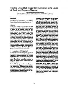
FIGURE 4.1. What Nyquist sampling really means: the smallest feature should be at least 4 pixels wide. In (A), a yellow beam scans over two red point features. Because the “resolution” of the micrograph is defined, by the Abbe/Rayleigh criterion, as the distance from the center to the edge of the beam while Nyquist sampling says that pixels should be one half this size, pixels are one quarter of the beam diameter. From this, it follows that, at the end of each line, the beam will move down the raster only 25% of its diameter (i.e., it will scan over each feature at least four times). In (B) we see how such a signal will be displayed as a “blocky” blob on the screen, about 4 pixels in diameter. Because our eyes are designed to concentrate on the edges of each pixel, the screen representation doesn’t look like an Airy disk (and would look even worse were we to add the normal amount of Poisson noise). We can get an “accurate” impression of the image of a point object only if we resample the 4 ¥ 4 array into a much larger array and apportion the detected signal among these smaller, less distinct, pixels to form an image that looks like the circular blob on the lower right.

An image of a preparation of circular nuclei 7 mm in diameter has spacings of all possible orientations that are equal to the diameter of the nuclei in micrometers. The inverse of this diameter, in features/mm, would be the spatial frequency of the nuclei (in this case, about 150/mm). The intensity of the CTF at zero spatial frequency is a measure of the average brightness of the entire image. The CTF graphs the image contrast assuming that the object itself has 100% contrast (i.e., that it is composed of alternating black and white bars having a variety of different periodicities; as few biological specimens have contrast this high, contrast in microscope images will be correspondingly lower). Because of the limitations imposed by diffraction, the contrast of the widest bars (spatial frequency near zero) will be almost 100% while bars that are closer together (i.e., have a spatial frequency nearer the diffraction limit) will be recorded with lower contrast in the image.

FIGURE 4.2. A properly sampled 2D image. When your image is recorded with Nyquist-sized pixels then the smallest features will be 4 to 5 pixels across. (This figure kindly provided by Dr. Alan Hibbs of BioCon, Melbourne, Australia.)

100% Rayleigh or Abbe resolution

The pixels as they appear in red channel of the display CRT

Digitally enlarged view (8x), showing individual image pixels.

Contrast

seen as pixels

or, as seen after re-oversampling, then smoothing

25%

0 0

R/4

R/2

R Spatial frequency

FIGURE 4.3. Contrast transfer function (CTF). This graph relates how the contrast of a feature in the image is inversely related to its size. Smaller “spacings” (see boxes below graph) have higher “spatial frequency” and will appear in the image with much lower contrast than they had in the object. Although the Rayleigh/Abbe resolution is conventionally set at the point where the CTF has dropped to 25%, even features that are twice this large (i.e., have one half the spatial frequency, R/2) are still represented in the image with only about half of their original contrast.

Points, Pixels, and Gray Levels: Digitizing Image Data • Chapter 4

From Figure 4.3, one can see that the Rayleigh-criterion resolution is not really a hard-and-fast resolution limit but merely the spatial frequency at which the CTF of the optical system has dropped to about 25%. In general, features twice as big as the Rayleigh limit (i.e., R/2, half the spatial frequency) will be transmitted with a bit less than twice this contrast (i.e., ~50%), and so on for progressively larger features (although the image contrast can never be more than 100%). One of the reasons that the CTF is such a useful guide to optical performance is that it emphasizes the performance for imaging small features. If we assume for a moment that we are using a high numerical aperture (NA) objective (NA 1.4) producing a Rayleigh resolution (R, in a microscope, this is often called the Abbe limit) of ~0.25 mm, then the part of the graph to the left of the R/4 marking describes the way that the optical system will transmit all the features larger than 1.0 mm (or R/4). All of the plot to the right of the R/4 mark refers to its transmission of features smaller than 1.0 mm. This is the part of the plot where problems are likely to occur. In addition, it reminds us that diffraction affects the appearance of features that are larger than the Abbe limit. In the end, resolution can only be defined in terms of contrast. It is NOT the case that everything works perfectly up to the Abbe limit and then nothing works at all. The reason that the CTF is particularly useful in microscopy is that, if everything goes right (i.e., proper illumination, optically uniform specimen, no lens aberrations), its shape is entirely determined by the process of diffraction. If this is true, then the curve is directly analogous to what we can see in the back-focal plane (BFP) of the objective lens. You may recall that, when illuminated by axial illumination, large features (which have low spatial frequencies) diffract light near the axis while smaller features diffract light at larger angles. If you imagine that the left axis of the CTF plot (zero spatial frequency) is located at the exact center of the BFP, then the sloping part of the CFT curve can be thought of as representing a radial plot of the light intensity passing through the rest of the BFP.2 Light passing near the axis has been diffracted by large features. As many diffraction orders from these features will be accepted by the NA of the objective, they will be represented in the image with high contrast (Fig. 4.4).3 Light out at the edge of the BFP consists of high-order diffraction from large features plus low-order diffraction from smaller features. The smallest features visible at this NA will diffract light at an angle that is almost equal to the NA of the objective, as defined by the outer border of the BFP. As only one diffraction order from these features will be accepted by the objective, the features that diffract at this angle will be represented in the image with low contrast. As a result, one can “see” important aspects of the CTF, simply by viewing the BFP, for example, using a phase telescope or Bertrand lens. For example, when using a phase lens for fluorescent imaging, the phase ring present in the BFP of the objective partially obscures (50%–90% opacity) and shifts the phase of any rays passing through it. Therefore, features in the object that are

61

the correct size to diffract at the angles obscured by the ring will be less well represented in the image data recorded. Finally, the CTF is useful because it is universal. Assuming that you normalize the spatial frequency axis of the CTF plot in Figure 4.3 for the NA and l in use (i.e., the spatial frequency under the 25% contrast point on the curve should be the reciprocal of the Abbe resolution), it is a reasonable approximation of the CTF of any diffraction-limited optical system. As such it defines the best we can hope for in terms of direct imaging (i.e., without non-linear image processing such as deconvolution to be discussed later, or the use of clever tricks like STED as discussed in Chapter 31, this volume). The CTF can be used to characterize the performance of every part of the imaging system: not only the optical system but also the image detector (film or video camera), the image storage system (film or digital storage), the system used to display or make hardcopy of the stored result, even the performance of your eyes/glasses! The performance of the entire imaging chain is merely the product of the CTF curves defining all the individual processes. Because the CTF always drops at higher spatial frequencies, the CTF of an image having passed two processes will always be lower than that for either process by itself (Fig. 4.5). In other words, small features that have low contrast become even less apparent as they pass through each successive stage from structures in the object to an image on the retina of the viewer. As can be seen from Figure 4.5, the steps with the lowest CTF are usually the objective and the video camera. A digital CCD camera (i.e., a CCD camera in which each square pixel reads out directly into a specific memory location) would produce better results than the video-rate television camera/digitizer combination shown in Figure 4.5 because the latter digitizes the data twice, a process that can reduce the contrast of fine, vertical lines that are sampled in the horizontal direction by a factor of 2. The performance of all of the steps past the ocular can be “improved” by

2

It is uncommon to image using only axial illumination, at least in part because filling the condenser BFP increases the number of diffraction orders that can pass through the objective, thereby doubling the resolution. It is assumed here only for illustrative purposes. 3 Strictly speaking, the following analysis is only accurate for axial illumination. However, even for the convergent illumination used to get the highest resolution in transmission imaging, the general point is correct: light rays carrying information about smaller features are more likely to be represented by rays that pass near the edges of the back-focal plane.

FIGURE 4.4. Relationship between the CTF and the position in the back-focal plane of the objective lens that axial light will diffract from features of different spatial frequencies.

Chapter 4 • J.B. Pawley

CTF of each, individual stage

use rasters of 512 ¥ 512 or 1024 ¥ 1024 pixels, although other dimensions are not uncommon. In scientific imaging, it is advisable to avoid digitizing schemes involving pixels that do not represent square subunits of the image plane (for example, those produced by digitizing each line from a television image into only 512 pixels rather than 640 pixels) as there is little support for displaying or printing such images directly.

contrast

62

spatial frequency

Cumulative CTF to this stage

Stages of microscopy

objective

occular

video camera

digitizer

hardcopy

FIGURE 4.5. The CTF of each component in the microscope system affects the final result. Every optical component and digital process can be characterized by a CTF. The effects of a series of steps can be determined by multiplying together the CTFs of all the steps.

working at higher magnification: if the pattern of light presented to the camera (or eye) contains larger features, their contrast will be reduced less by imperfections in the camera (or eye) itself. However, this approach also has limitations. Working at higher magnification requires either a larger image sensor or a smaller field of view. Much of the remainder of this chapter is concerned with making the most appropriate choice of “magnification,” although the discussion is usually in terms of “How large should a pixel be, referred to the object?” Once the information is digitally encoded, further CTF degradation can be minimized as long as certain rules are obeyed (as discussed below and in Chapter 48, this volume). The lessons so far are

• No matter how high the contrast of the optical process defin•

ing a feature in the object, smaller features are always depicted in the final image with less contrast than larger features. Features that have low intrinsic contrast in the object will have even lower contrast in the image.

On the other hand, remember that Figure 4.3 shows the best for which we can hope. It is not at all hard to end up with system performance that is substantially (~50%) worse than that described by Figure 4.3. This means that while one can no longer see the smallest features, one now might just as well use larger pixels. In this chapter, we will assume that Figure 4.3 really does describe optical system performance, and go on to consider the other factors important to ensure that image data is digitally recorded in an optimal manner.

DIGITIZATION AND PIXELS Image digitization refers to the process whereby an apparently continuous analog image is recorded as discrete intensity values at equally spaced locations on an xy-grid over the image field. This grid is called a raster. Typically the image area is divided into an array of rows and columns in much the same way as a television image. In North and South America and Japan, the television image is composed of 483 lines covering a rectangular area having proportions that are 3 units high by 4 units wide. If each line in such an image is divided into about 640 equal picture elements or pixels, then each pixel will be square if you discard three lines and record a raster of 640 ¥ 480 pixels. Newer computer-based CCD image digitization systems do not rely on any broadcast television standard, and are more likely to

Digitization of Images The actual process by which the signal from the image detector is converted into the intensity values stored in the computer memory for each pixel depends on the type of microscope involved. CCD cameras: Typically, a widefield or disk-scanning confocal microscope uses a camera incorporating a CCD image sensor. Although we will not describe in detail the operation of these sensors (see Chapter 12 and Appendix 3, this volume), the camera operates by reading out a voltage proportional to the number of photons absorbed within a small square area of the sensor surface during the exposure time. As long as the intensity value readout is stored directly into the computer, this small area on the CCD defines the pixel size for the remainder of the imaging system.4 As far as the user is concerned, the most important parameters involved in attaching the CCD to the microscope are the NA of the objective, the wavelength, and the total magnification up to the surface of the sensor. Together these parameters determine both the proper size of a pixel referred to the plane imaged in the specimen, and also the optimal pixel size for the CCD. For example, if a CCD camera with 8 ¥ 8 mm pixels is coupled to a microscope with a 40 ¥ 1.3 NA objective via a 1¥ coupling tube, each sensor pixel will cover 8/40 = 0.2 mm. The same camera and coupling will produce “0.08 mm pixels” when used with a 100¥ objective, but the number of photons striking each pixel during a given exposure time will now be 2.5 ¥ 2.5 = 6.25¥ less because signal intensity goes down with the square of the magnification. Photomultiplier tubes (PMTs): On a laser confocal microscope, signal photons strike the photocathode of a PMT where some small fraction of them each produce a single photoelectron (PE). These PE are then amplified about a million times by charge multiplication. The signal current emerging from the PMT is digitized under the control of a pixel clock which also controls how the scanning mirrors sweep over a rectangular raster on the specimen. This clock divides the time taken to scan one line into the appropriate number of intervals, so that each time interval represents a square area of the image (i.e., each time interval represents the same distance along the scan line as the spacing between adjacent lines). As the PMT signal is digitized for each interval, or pixel, the pixel value represents the signal intensity of a small square area of the final image. Because the shape of the raster in a laser confocal microscope is defined by the size of the electronic signals sent to the scan mirrors (Fig. 4.6) rather than by the fixed array of electrodes on the surface of the CCD, there is much more flexibility in terms of the size and shape of the rasters that can be scanned.

4

This is not true if the CCD is read out to form an analog “composite video” signal which is then redigitized into the computer. Such uncorrelated redigitization can reduce the effective horizontal resolution of the data by almost a factor of 2 and should be avoided. Likewise, one should be careful when “resizing” images using image processing programs because, unless it is done in integer multiples, this process also involves resampling, a process that reduces image contrast.

Points, Pixels, and Gray Levels: Digitizing Image Data • Chapter 4

63

FIGURE 4.6. Mirror scan angle and magnification. The galvanometer mirror scans the laser beam across the focus plane of the objective by effectively changing the angle at which the laser beam passes through the back-focal point of the objective lens. A larger deflection of the mirror scans the light over a longer line on the specimen (B). As the data from this longer line are finally displayed on the same sized computer monitor, the effect is to lower the overall magnification of the image. If the number of pixels digitized along each line remains constant, a longer line on the specimen implies larger pixels.

A

In particular, a combination of the magnification of the objective and the zoom magnification on the scan control panel defines the dimensions of the raster at the object plane in the specimen. If more current is sent to the scanning mirrors (low zoom magnification), they will drive the scanning beam over a larger area of the specimen and, assuming a fixed raster size (e.g., 512 ¥ 512 pixels), this means that each pixel will now represent a larger area of the specimen (Fig. 4.7, darkest square). Conversely, higher zoom magnification will send smaller currents to the scan mirrors. This will make the raster scan over a smaller area on the specimen, and make the area represented by a single pixel proportionally smaller (Fig. 4.7, lightest square). As a result, and unlike the CCD case, pixel size is under continuous control as the user changes raster shape/size and zoom magnification settings. However, your control panel should constantly display the current pixel dimensions.

Zoom 4x, 512 × 512

Zoom 2x, 512 × 512 Zoom 1x 512 × 512

FIGURE 4.7. Relationship between zoom setting and area scanned on the specimen. A higher zoom magnification setting scans the beam over a smaller area of the sample. As each pixel now represents a smaller area on the specimen, we say that the pixels are “smaller.” The important thing is to adjust the zoom magnification so that the pixel size is about 50% of the Abbe resolution for the NA and wavelength in use.

B

HOW BIG SHOULD A PIXEL BE? SAMPLING AND QUANTUM NOISE Clearly, it is not possible to represent features spaced, say, 1 mm apart if the pixel dimensions are 2 ¥ 2 mm. Having smaller pixels will increase the chance that small features of the specimen are adequately sampled. However, having smaller pixels also has disadvantages. It means either imaging a smaller area of the specimen or using a larger raster size [1024 ¥ 1024 rather than 512 ¥ 512; Fig. 4.8(A)]. If you choose a larger raster, you must store and analyze more data. You must also either collect fewer signal photons from each pixel [Fig. 4.8(B)] or take longer to scan the larger raster. Longer counts require you to expose the specimen to more light [Fig. 4.8(C)], a process that may be deleterious, especially to living specimens. Settling for less signal in each pixel is also not without problems. The signal that is being counted is not continuous but is composed of photons, sometimes quite small numbers of photons. In fact, it is not uncommon for the signal from a single pixel in the bright area of a fluorescent confocal specimen to represent the detection of only 9 to 16 photons. As the detection of a photon is a quantum mechanical event, there is an intrinsic uncertainty in the number actually detected on any given trial. This uncertainty is referred to as Poisson, or statistical, noise and is equal to the square root of the number of events (photons) detected. Therefore, reading 16 photons really means detecting 16 ± 4 events.5 Like diffraction, Poisson noise is a rigid physical limitation. The only way to reduce the relative uncertainty that it causes is to count more events. If we increase the zoom magnification by a factor of 2, there will be 4¥ as many pixels covering any given scanned area of a two-dimensional (2D) specimen. If, at the same time, we also reduce the laser power by a factor of 4, the same total amount of signal/mm2 will emerge from the reduced area now being scanned, producing the same bleaching or other photo damage but the average signal level in each bright pixel will now be not 16 photons, but only 4 ± 2 photons. The uncertainty of each measurement is now 50%. In other words, when photons are scarce, one seldom wants to use pixels smaller than are absolutely necessary to record the information in the image. It is simply a case of “winning on the swings what you lose on the roundabouts.” Either scenario has advantages and dis5

That is, 67% of a series of measurements of this intensity would be in the range of 12 to 20 photons and 33% of such measurements will be outside even this range. In other words, if you detect 10 photons you really have very little idea about what the signal intensity really “should have been.”

64

Chapter 4 • J.B. Pawley FIGURE 4.8. Relationship between raster size, pixel size, and “light dose.” (A) If a microscope scanning at a zoom setting of 1 is switched from a 512 ¥ 512 raster to one of 1024 ¥ 1024 pixels, the dimensions of each pixel on the specimen will drop by 50%. (B) If the same amount of signal is split between more pixels, the signal level from each one goes down (and the Poisson noise goes up), but if the beam scans more slowly or is made more intense so that the same amount of signal is still collected from each pixel, (C), then the amount of damage/pixel increases. There is no free lunch!

512 × 512

1024 × 1024

A

B 16

4

1

photons/pix

16 photons/pix

C 16

64

256

total photons

advantages. Surely there must be a “best” strategy for setting the zoom correctly to produce the best pixel size. Fortunately there is!

THE NYQUIST CRITERION It was not until 1929 that Harry Nyquist, who worked for the telegraph company, gave much thought to the optimal strategy for digitally sampling an analog signal (Nyquist, 1928). When such sampling first became technically possible, the signal in question was electronic, perhaps the audio signal of a radio program. The process envisioned, as diagramed in Figure 4.9, requires six components: a pre-amplifier feeding the signal to the analog-todigital converter (ADC), a digital memory system for storing the digital data from the ADC, a digital-to-analog converter (DAC) that reassembles the digital information into a continuous analog signal that can be passed to the output amplifier, and, finally, a clock to synchronize the whole process. The clock determines the time interval between samples (i.e., the sampling frequency, in samples/s). The information content of any electronic signal is limited by the electronic bandwidth of the amplifier used to transmit it.6 In 6

Think of this as the frequency response of your stereo system. Good high frequency response will let you hear your music more accurately. The frequency response of your stereo is usually plotted in decibels (a measure of relative power) on the y-axis against the log of the frequency on the x-axis. Note the similarities to Figure 4.1.

1949, Claude Shannon was able to prove Nyquist’s theorem and show that, if the interval between the intensity measurements is less than half the period of the highest frequency in the signal, it will then be possible to faithfully reconstruct the original signal from the digital values recorded (Shannon, 1949). The Shannon sampling frequency, which is the inverse of the Shannon sampling interval, is also known as the Nyquist frequency, especially in the imaging community. It is often forgotten that there is a second part of the Shannon/Nyquist theorem: the part about reconstructing the original data. The theorem states that the output “amplifier” through which you play back the reconstructed signal from the DAC must have the same bandwidth as the pre-amplifier that originally fed the signal to the ADC. This is an important condition, one that is often not satisfied in current confocal microscopes unless their images are deconvolved before presentation (as will be discussed later). Attempting to apply Nyquist sampling to 2D or threedimensional (3D) images gives rise to the question: How do we measure the “bandwidth” of the “amplifiers” when faced with the problem of digitizing 2D or 3D microscopical image data? Electronic bandwidth is not a simple concept. The frequency response of any real amplifier does not remain flat until some frequency and then go abruptly to zero at any higher frequency. Rather, limitations imposed by the components of which the circuit is made cause its power response to decrease gradually as the frequency increases, usually dropping to one half or one quarter the original output power as the frequency goes up each octave above

Points, Pixels, and Gray Levels: Digitizing Image Data • Chapter 4 FIGURE 4.9. The components needed to digitize and reconstruct an analog signal. The “post-amp” is essential to remove the “single-pixel noise” that is added to the original analog signal by Poisson statistics. Because real, Nyquist-sampled data can never have features smaller than 4 pixels across, single-pixel noise can be removed by limiting the bandwidth of the post-amplifier. In microscopy, this limiting function is implemented by either Gaussian filtering or deconvolving the raw 3D data.

Original signal

PreAmp

Digitized signal

Analog to digital converter (ADC): digitizes signal into 0s and 1s

Digital memory: stores signal intensity at times defined by clock

Reconstructed signal

Digital to analog converter (DAC): makes analog signal from 0s, 1s

PostAmp

Digitizing Clock

Digitized signal

Original NOISY signal

65

A Reconstructed signal

B

some “cut-off frequency.”7 As in optical systems, higher electronic frequencies are still transmitted, but at lower intensity. In electronics, the convention is to define the bandwidth by the frequency at which the power response drops to 50% of the linear response, a frequency called the “3 dB point.” This defines the bandwidth Shannon used. In optical terms, we usually think of the image being useful until it drops to about 25% of its peak contrast (i.e., the Abbe criterion noted above), although this too is an arbitrary choice. If we think of an analog electronic signal as a one-dimensional image, it is not hard to think of an image as a 2D (or 3D) version. Except that image data varies in space rather than time, the rest of the analysis applies. The “bandwidth” of an image must be somehow related to its “sharpness,” and this is related to the highest spatial frequencies it contains. Now if we were applying this analysis to the CCD sensor used in a consumer snapshot camera, we would have a problem. Although the “world” out there may be composed of objects of every size, we really have little knowledge of the CTF of the lens, let alone whether or not it is focused correctly or whether you are capable of holding it motionless during the exposure period. As a result, we really don’t know the bandwidth of the data and consequently we don’t know whether or not the pixels are small enough to meet the Nyquist criterion. “More is better” is the slogan that sells. Fortunately, this is not the case in microscopy. Here we do know that, at the very least, diffraction limits the maximum sharpness of the data that can be recorded, and that the “spatial frequency response” of the microscope can be defined by a suitably calibrated version of Figure 4.3. Therefore, the convention is to choose the size of the pixel to be equal to one half of the Abbe criterion resolution of the optical system. There are some caveats. The structural features of a 1D image can only vary in that dimension. The structural features of a 2D image can vary in more than two possible directions. Although signals defining features such as vertical or horizontal lines, vary

7

As in music, an octave represents a factor of 2 in signal frequency.

in only the x- or y-directions, respectively, what about a set of lines oriented at 45° to these axes? It would seem that sampling points along a 45° line would be spaced 1.41¥ as far apart as sampling points along features that vary along the x- or y-axes. Pixels just small enough to sample a given small spacing when it is oriented vertically or horizontally would be 1.41¥ too big to sample this same structure were it to be oriented at 45°. However, this analysis neglects the fact that all image “features” extend in 2D. As a result, lines running at 45° will also be sampled by other pixels in the array and if we count all the pixels that sample the blurred features along a line at 45°, one finds that the sampling interval isn’t 1.41¥ larger but in fact only 0.707 as large as the sampling interval in the x- or y-directions (Fig. 4.10). Clearly we want to be able to see structures oriented in any direction. To be on the safe side, it may be better to use pixels ~2.8¥ smaller than the finest spacing you expect to record in your image.8

Estimating the Expected Resolution of an Image Assuming that the shape of the CTF curve describing the optics of the microscope depends only on the NA and the wavelength, it is also a plot of power level versus the logarithm of the frequency, just like the frequency response curve of a stereo. Although the CTF defines the best that one can hope for, it does not guarantee it. Performance can be worse, and if, in fact, it is worse, does it make sense to use smaller pixels than we need? Let us take some concrete examples. The calculation of the Abbe criterion resolution assumes that two point objects of similar intensity are represented in the image as Airy disks, spaced so that the peak of each is located over the first dark ring of the other. If we sum the light intensity of these two Airy disks, there will be a valley between the two peaks in the summed image. At the exact mathematical bottom of this valley, the intensity is

8

A similar line of argument could be used to suggest that one use even smaller pixels when sampling 3D data because the diagonal of a cube is 1.732x longer than its side. However, we will soon see that, as the z-resolution of the confocal microscope is always at least 3x lower than the xy-resolution, ignoring this factor does not cause any problem in practice.

66

Chapter 4 • J.B. Pawley

0. 71

x

d 25%

1. 41

x

Rayeigh resolution, d, and Nyquist digitizing FIGURE 4.11. Nyquist sampling of an image of two points separated by the Rayleigh resolution.

y x

x

FIGURE 4.10. Spatial frequency and geometry. The 3 ¥ 3 array of squares represents a small raster and the dots in the center of each represent the sampling points. Although one might be tempted to think that these sampling points would be too far apart along the diagonal to be able to properly sample any signal that just meets the Nyquist sampling criterion when oriented either horizontally or vertically, this is not so because the sampling points of the adjacent diagonal rows of pixels actually sample at 0.71 of the x- or y-raster pitch.

about 25% lower than the intensity of either peak. This is the basis of the idea that 25% contrast is equal to the Abbe criterion resolution (Fig. 4.11). Under these circumstances, the smallest resolvable spacing is defined as the distance between the center of an Airy disk and the center of its first dark ring. To be properly sampled, pixels should be less than one half this distance in size.9 Suppose that, along a line joining centers of the images of the two points, one pixel just happens to be centered on the brightest part of one Airy disk. The adjacent pixel would then be centered over the valley between the peaks and the third pixel will be over the second Airy peak. If we sample the brightness at the center of these three pixels, the digital data will reflect the trough in intensity between them. On the other hand, if the “valley pixel” has a value proportional not to the intensity at the exact center of the pixel but to the average intensity over the whole pixel,10 the value stored for the center pixel will be much more than 75% of the peak intensity:

9

Or perhaps a bit less if we use the 2.3 or 2.8 samples/resolvable element (resel) suggested above. For simplicity, I will stick to 2 samples/resel in this discussion, because, as discussed below, in the case of the fluorescent images of most interest, lack of signal usually prevents one from realizing Abbe criterion resolution and consequently the “actual” resolution is lower than Abbe and using somewhat fewer/larger pixels is appropriate. 10 In microscopy terms, the CCD samples the average value of a pixel while the ADC sampling the PMT signal in most single-beam confocals acts more as the center-sampling device.

that is, the contrast recorded between the three pixels will now be much lower than 25% (Fig. 4.12). If the two features that produced the two Airy disk images are not of equal brightness (surely the more likely occurrence) then the contrast along a line joining the peaks will again be much less than 25%. Worse still, what if the peaks are uncooperative and are not squarely centered on two pixels, nicely spaced on either side of the central, darker pixel? If the value recorded at each pixel is the average of the intensity across the pixel, the contrast along a line between the features can be substantially reduced or even eliminated (Fig. 4.13). Now it is fair to say that while these considerations are problems, to some extent, they only represent a serious problem if we ignore the second part of the Nyquist sampling theorem, the part having to do with reconstruction. If the image is properly reconstructed (deconvolved), in most cases, information from adjoining pixels (those in the rows in front or behind the printed page in Fig. 4.13) will allow one to smooth the image to form a good estimate of the structure of the original object as is discussed later in the chapter.11 Deconvolving or filtering the image data eliminates high spatial frequencies. Effectively, such filtering causes the signal to overshoot the contrast present in the digital signal. This process substantially reverses the apparent reduction in contrast that occurs on digitization.

11

Periodic structures having a size near the resolution limit also present sampling problems. Suppose that the object is a sinusoidally varying structure with a period equal to the Abbe spacing. If the two samples required by Nyquist coincide with the plus and minus excursions of the sine wave, then we will have some measure of its magnitude and the position of its zerocrossing [Fig. 4.5(B)]. However, if the two samples happen to be taken as the sine wave crosses its origin, all the sampled values will be zero and hence can contain no information about the sine wave [Fig. 4.5(C)]. This apparent exception to Nyquist sampling success is not actually an exception in terms of the original application of the theorem: information theory. According to information theory, a sine wave contains no information beyond its frequency and magnitude. As long as you have slightly more than two samples/period, the sampling intervals will “beat” with the data to create a sort of moiré effect, from which one can estimate the magnitude and period of the sinewave object. All this does not change the fact that an image of a periodic object must be at least 2x over-sampled if it is to be recorded with reasonable fidelity [Fig. 4.5(A)]. This is particularly important when imaging the regular patterns found on resolution test targets.

Points, Pixels, and Gray Levels: Digitizing Image Data • Chapter 4 FIGURE 4.12. Two methods of sampling: at the center point and as the average value.

67

Nyquist digitizing of two point objects at Abbe separation.

12%

25%

A

Center sample

B

Average sample

Nyquist digitizing of two point objects at Abbe separation with center sampling.

25%

FIGURE 4.13. How can this possibly work? “Lucky” and “unlucky” Nyquist sampling of the image of two points separated by one Rayleigh resolution.

“lucky”

On the other hand, this reduction in contrast is entirely relevant if one tries to assess raw digital image data from a Nyquistsampled confocal microscope directly from the cathode-ray tube (CRT) or liquid-crystal display (LCD) screen or when viewing unprocessed data as a hardcopy from a digital printer. There is another problem that even proper reconstruction will not solve. Recall the example above in which a “bright” signal (perhaps the peak of an Airy disk?) was only 16 ± 4 photons. Clearly the ±4 represents a 25% average error, that is the same order of uncertainty as the maximum expected contrast we hope to see between the peaks (Fig. 4.14). In other words, even though diffraction theory says that we should record a lower signal in the

“unlucky,” no dip

A

B

pixel between two peaks of equal intensity, at these low signal levels, Poisson statistics says that, about 30% of the time, the intervening pixel will actually be measured as brighter than at least one of the two peaks. [As each peak pixel is subject to its own independent statistical variations, in a given image, it is unlikely that all 3 pixels (or 9 pixels if we consider the 2D image) will be recorded as the same brightness.] Artifactual “features” such as those diagramed in Figure 4.14(B) and produced by “single-pixel” Poisson noise, will be removed if the dataset is deconvolved or even 3D-Gaussian smoothed as discussed below.

Abbe spacing FIGURE 4.14. The effect of Poisson noise. While a Nyquist-sampled signal of Rayleigh-separated features seems to work well when the signal is composed of many photons and has little noise (A), when the number of photons counted drops by a factor of 100, and the signal-to-noise ratio (S/N) drops by a factor of 10, then random variations in the signal can play havoc with the data (B) allowing “single-pixel” noise features to masquerade as very small features.

500

5

Many counts

A

Few counts

B

68

Chapter 4 • J.B. Pawley

The Story So Far

Under-Sampling?

Once we know the size of the smallest data we hope to record, we can adjust the zoom magnification on a confocal microscope or the CCD camera coupling tube magnification on a widefield microscope to make the pixels the right size. But is Figure 4.3 really a good way to estimate this maximum spatial frequency?

In some cases, the useful resolution of the image is set by nonoptical limits. An example might be a fluorescence image of a cell containing a dye that changes its properties in response to the concentration of certain ions. If the diffusion of ions and dye molecules precludes the existence of small-scale variations in the fluorescence signal from such a cell (i.e., no small features), there is no need to divide the data into small pixels. Measuring each of fewer, larger pixels for a longer time may give more accurate results, especially when the expected changes in ion concentration produce only small changes in the fluorescent properties of the dye used (i.e., a low-contrast image) or when two noisy images must be ratioed to obtain the final result. In such specimens, high spatial resolution is impossible because of diffusion, while high intensity resolution is required to make small changes visible. In this case, it is particularly important to spatially filter the raw digital data before attempting to display or ratio the data (see Chapter 42, this volume).

REALITY CHECK? Are we kidding ourselves in thinking we will be able to see individual point features separated by Abbe criterion resolution when viewing faint, fluorescent specimens? In fact, under these conditions, we may be lucky to separate features that are even twice this far apart and we now recognize that we could record such data using pixels that were twice as big and 4¥ less numerous (in a 2D image; 8¥ fewer in a 3D image). On the other hand, our human ability to “see” (recognize?) extended features, such as fibers or membranes, is enhanced by the ability of our mind to extract structural information from noisy data. We do this “magic” by integrating our visual analysis over many more pixels (100¥?). While viewing noisy, extended objects doesn’t improve the quality of the data, it allows the mind the illusion of averaging out the statistical noise over more pixels because each is an independent measurement. In this case, Nyquist/Abbe sampling may be more worthwhile after all.

Is Over-Sampling Ever Wise? Yes! When viewing a specimen that is not damaged by interacting with light, over-sampling can improve visibility by recording more data and hence reducing the effect of Poisson noise. Videoenhanced contrast microscopy has been utilized to image isolated features much smaller than the Abbe limit. When imaging structures such as isolated microtubules, one often employs “empty magnification,” sampling much more finely than is required by Nyquist. This is effective because such structures produce only a very small amount of image contrast. As a simplified example, assume that the signal from the feature is only 1% greater than that from the gray background. Turning the light signal into an electronic signal permits one to adjust the contrast arbitrarily. However, if the electronic signal is too noisy, the result will just be more contrasty noise. To detect a 1% difference using photons, we must ensure that the contrast produced by Poisson noise variations in the background gray are less than that between the background and the feature. At the minimum, this involves counting at least 10,000 photons/pixel because the Poisson noise is 10, 000 and 100/10,000 = 1%. One could produce an even more easily interpretable image if the intensity of the feature differs from the background by more than one standard deviation. Recording 100,000 photons/pixel would make the 1% signal become 3¥ more than the Poisson noise. As most image sensors saturate (become non-linear) when exposed to more than 100,000 photons/pixel, the only way to “see” such a low contrast feature is to make many different measurements (i.e., use more pixels). A single pixel might be bright because of statistics but it is less likely that four adjacent pixels will all be recorded as bright. Using more pixels produces even greater visibility by further separating the signal representing the feature from that representing the background.12

DIGITIZING TRADE-OFFS We have now discussed how most of the relevant factors: pixel size, optical resolution, and photon signal strength all interact. The best choice will almost always depend primarily on the robustness of your sample: Assuming careful adjustment of the optics, more counted photons will always give a better estimate of the distribution of fluorescent molecules within the specimen. You must decide when the need for better spatial or intensity resolution justifies increasing the signal level and when it cannot be tolerated because to do so would reduce the “biological reliability” of the data (i.e., kill or injure the cells, see Chapters 38 and 39, this volume). Data with higher spatial resolution may not be useful if they represent structural features of a cell that is dead or dying.

NYQUIST RECONSTRUCTION: “DECONVOLUTION LITE” Elsewhere in this volume the technique for recording 3D data sets of both point objects and fluorescent specimens using a widefield microscope and a CCD camera and then computer-processing the resulting data to produce 3D images much like those produced by the confocal microscope are discussed in detail (Chapters 23, 24, and 25). The most advanced form of this processing is called iterative, constrained 3D deconvolution and uses the image of the point object to determine the 3D point-spread function (PSF) for the imaging system. Here, I will discuss only one part of this process, a process that can be thought of as filtering or smoothing.

12

It is important to state here that I am not talking about limitations in the image that could be overcome by resetting the “contrast” and “brightness” of the image display system in order to make any image contrast more visible to the observer. These are assumed to be set in the best possible manner for the individual concerned. The limitation on visibility discussed here relates solely to the fact that the data in the recorded image is insufficiently precise for any observer (or even a computer!) to determine the presence or absence of the structure. For more about visibility and the Rose criterion, see Chapters 2 and 8, this volume.

Points, Pixels, and Gray Levels: Digitizing Image Data • Chapter 4

As noted above, sampling the analog data to produce the digital record was only half of the process. The second part involves “passing the reconstructed signal through an amplifier having the same bandwidth as that from which the original data was received.” To see why this is necessary it may help if we imagine a reconstruction of the digital data as being sort of a bar graph, in which each bar represents the intensity value stored for this pixel [Fig. 4.15(A)]. Clearly a “signal” represented by the boxy contour line going along the tops of the bars will generally change much more abruptly than the original data. As a result, it is not a faithful reconstruction of the original signal. How can it be made more similar? In terms of Fourier optics a “square-wave object,” such as a bar, can be thought of as being composed of the sum of a number of sine-wave objects, each having a periodicity that is an integer-multiple (harmonic) of the square wave frequency. The first sine term in this series converts each “square” of the square wave into a rounded curve. As subsequent terms are added, they add the “ears” to the hump that make the sum resemble the original boxy square wave ever more accurately (Fig. 4.16). If we apply this logic to the top line of our bar graph, we can think of it as the sum of a lot of sine waves. If we leave out the higher harmonic terms before reconstructing the original line, the boxy corners will be rounded. Passing the boxy reconstruction through an amplifier of limited bandwidth prevents the higher order terms (higher frequencies) in the sine-wave series from being included in the reconstructed signal [Fig. 4.15(C)]. This is important when viewing a digital image because our eye/brain system is designed to emphasize the sharp edges that define the boundary of each pixel on the liquid-crystal display (LCD) screen and this is more likely to happen when a single noisy pixel stands out from a darker background. The same thing is true when we reconstruct an image from digital data. However, in the case of fluorescence or other lowintensity data, there is an additional complication. The Nyquist theorem assumes that the signal digitized is continuous, that is, that

A

B

69

original square wave

order 1 and 3

first 3 terms order 1 red order 3 green order 5 blue

order 1 through 5

order 1 through 23

FIGURE 4.16. Fourier analysis. The Fourier theorem says that any periodic structure (such as the “square-wave” in the top left) can be represented as the sum of a number of sine waves, each of which is harmonic of the frequency of the structure. Think of these frequencies as the spatial frequencies introduced in Figure 4.2. As more components are added to the sum, the result looks more and more like the original. The same thing happens in microscopy, where using a lens with a higher NA allows more “terms” that are carrying high-frequency information (and therefore diffract at higher angles) to contribute to the image.

determining the intensity to be stored for each pixel does not involve measuring small numbers of quantum-mechanical events. A continuous signal is not capable of changing by a large amount from one pixel to the next because the pre-amplifier bandwidth was too narrow to permit such a rapid change. In the microscopic case, the Abbe bandwidth limits the amount of change possible between adjacent Nyquist pixels. However, in the confocal, Poisson noise can effectively sneak past the “preamp”13 and get digitized as part of the signal. As a result, such abrupt changes can be recorded. Consider the following example: Suppose we record the image of a bright point object on a black background using Nyquist sampling. A one-dimensional (1D) transect across the center of this feature might include 5 pixels. If sampled many times, the average recorded intensities in the central pixels might represent 10 photons, 8 in the pixels on either sides, and 3 for the two pixels next farther out. Had we recorded these averaged values, we would only have to worry about the “boxy corners” artifact noted above. However, if we only record a single set of values, Poisson noise introduces another factor. On any particular sampling of this line of data, we will generally not get the average values but something else. Were we to record not 3, 8, 10, 8, 3 but 2, 7, 13, 10, 4, the resulting reconstruction would now be very different. In particular, the center of the feature would have moved right and it would now appear narrower. The transients caused by the statistical nature of the signal have made a proper reconstruction more difficult. In fact, one would be correct in saying that, as the accuracy of the values stored in the computer are always limited by the statistics involved in counting quantum mechanical events, we can never know their “true” intensity of any pixel and our efforts

C FIGURE 4.15. How “limiting the bandwidth of the output amplifier” smooths off the rough corners (B) and improves the reconstruction (C).

13

This is possible because, in this case, it is the microscope optics that limits the bandwidth rather than an electronic pre-amplifier.

70

Chapter 4 • J.B. Pawley

to make a reconstruction of the object are doomed to be only approximate. While this dismal analysis is correct, we would like at least to make this approximation as accurate as possible. We can do this by applying the second Nyquist constraint: treating the data stored in the image memory to make sure that they do not contain spatial frequencies that are higher than the optical system could have transmitted. Although the best way to do this is to subject the 3D data set to iterative 3D deconvolution, much benefit can be gained by applying a simple 2D or 3D Gaussian smoothing filter. The effect of such a filter is to make the intensity of every pixel depend to some extent on the intensity of 63 or 124 neighboring voxels (depending on whether a 4 ¥ 4 ¥ 4 or a 5 ¥ 5 ¥ 5 smoothing kernel is used). This filtering effect averages out much of the statistical noise, reducing it by an amount proportional to the number of voxels in the convolution kernel. If we apply a smoothing filter that simply suppresses “impossible” spatial frequencies (i.e., those higher than the optical system is capable of producing), the contrast of small features that owe their (apparent) existence solely to the presence of quantum noise in the data will be greatly reduced. It is important to note that applying such a filter will reduce the apparent contrast of the image data. Digital look-up tables can be used to increase the apparent contrast on the viewing screen and the resulting images will be just as contrasty and will show less statistical noise than the raw data. MORAL: Your image is not suitable for viewing until it has been at least filtered to remove features that are smaller than the PSF, or, thought of the other way, to remove data having spatial frequencies beyond the maximum bandwidth of the optical system in use.

Some Special Cases In classic sampling theory, the time (or space) taken to measure or sample the intensity in each pixel is very small compared to the inter-pixel sampling interval. Although this condition is met for the ADCs used in commercial confocal microscopes,14 it is not met for the CCD camera, where it is common for the sensitive area of 1 pixel to be almost equal to the area it covers on the silicon surface. Clearly, this means that the space taken to sample the light flux is almost the same as the pixel size. The system works well enough as long as we stick to Nyquist sampling of a signal of known bandwidth (4–5 pixels/blob). In fact, some CCD manufacturers have gone even further and made an effort to increase the effective spatial resolution of a CCD by making a series of four or nine exposures, in which for each member of the series the sensor is offset from the previous one by one half or one third of a pixel in x and y, respectively.15 While reasonable results can be obtained in this way, problems can develop when it is applied to color imaging systems that employ a color pattern mask on each pixel (Fig. 4.17). Even in the confocal microscope, problems can occur because the zoom magnification control creates a variable relationship between the optical bandwidth of the signal and the electronic bandwidth which is set by the “time-constant” of the pre-amplifier just before the ADC. Not only that, but the optical bandwidth creates blurring in 2D while the pre-amplifier time constant only

14 15

Common values might be pixel period = 1 ms, sampling interval = 3 ns. For example, the Zeiss Axiocam.

Oversampling vs. “Duplicate and Smooth”

1.5/ 1300

1.5/ 1300 Triple Pixels use Photoshop “blur more”

Oversampled

.5/ 3900

.5/ 1300 Triple Pixels use Photoshop “blur more”

1.5/ 3900

FIGURE 4.17. Wiggling the chip to increase the resolution. A number of CCD cameras increase their effective spatial resolution by adding together the information from a set of four (or nine) images, each of which is collected with the CCD displaced horizontally by one half (or one third) of a pixel, first in x, then in y, compared to the other members of the set. The image in the top left was made at a tube magnification of 1.5¥ with the camera readout normally, while that below it was made with 3¥ less optical magnification and 3¥ more “resolution” by moving the chip. Both look quite similar when they have been upsampled and then blurred in Photoshop except that the “wiggled” result has a color caste caused by the fact that the color mask filters on the chip have a “pitch” that is twice the nominal pixel spacing. The up-sampled and blurred picture on the right is analogous to the round, red feature in Figure 4.1.

limits the signal bandwidth in the fast scan direction (usually horizontal). If the zoom is set to under-sample high-contrast optical data, then very large pixel-to-pixel variations are possible and the bandwidth should be wide. The reverse is true for over-sampling. In response to this problem, some commercial instruments estimate the optical resolution from the NA of the objective and the wavelength of the laser and then use this information to set the pre-amplifier to the optimal time constant (bandwidth) on the basis of the zoom setting. When such a system is functioning properly, the “apparent noisiness” of the signal recorded from a bright but relatively featureless object will become less as the zoom is increased: the signal/pixel remains the same but the longer time constants effectively averages this noisy signal over more pixels in the horizontal direction. Starting with the MRC-600, all Bio-Rad scanners used fullintegration digitizers. These were composed of three separate sections. At any instant, one is integrating the total DC signal current from the PMT during a pixel, the second is being read out, and the third is being set back to zero. This system effectively emulates the image digitizing system of the CCD. This approach works well for under-sampled data and was a great improvement on earlier systems that used a time constant that was fixed at (pixel time/4) and therefore let a lot of high-frequency noise through to the ADC. If you don’t want to worry about any of this, stick to Nyquist!

Points, Pixels, and Gray Levels: Digitizing Image Data • Chapter 4

GRAY LEVELS, “NOISE,” AND PHOTODETECTOR PERFORMANCE When an image is digitized it must be quantized in intensity as well as in location. The term gray level is the general term referring to the intensity of a particular pixel in the image. Beyond this general definition, things become more complicated. What kind of a measure? Linear? Logarithmic? What is a gray level? Let us begin at the beginning with a discussion of how these matters were handled by the first reliable method for recording image intensity: photography.

Optical Density Early work on the quantification of image intensity was related to the performance of photographic materials. Developed photographic emulsions are darker where they have been exposed to more light. However, this darkening process is not linear because the individual grains of silver halide that make up the emulsion only become developable after absorbing, not one, but two light photons within a short space of time (~1s).16 As a result, at low exposures the number of grains exposed is proportional to the square of the light intensity, a term we will use here to represent the number of photons per unit area per unit time at the detector. The photometric response of photographic emulsions is quantified in terms of so-called HD curves. These plot the log of the light intensity (H) against the log of the darkening (D). Figure 4.18 shows the important features of such a curve. The darkening is measured as a ratio compared to a totally clear film, using logarithmic optical density (OD) units: OD = 0 implies no darkening and all the light is transmitted; OD = 1 means that the emulsion transmits 10% of the incident light; OD = 2 implies that it trans-

5 Log optical density, (D)

4

Same emulsion w/longer development higher contrast Saturation

3

71

mits 1% of the incident light, etc. The use of a log/log scale allows one to describe the HD response over 4 to 5 orders of magnitude on a single plot. However, it also obscures much of the quantitative complexity of the plot and parts of it that seem “linear” would not seem so on a linear plot. Because there is always some background exposure of the emulsion, D is never “zero” but starts at the “fog” level. Small exposures produce almost no additional darkening because few grains receive two hits. Eventually, however, the log of darkening seems to become proportional to the log of exposure and the response curve enters its “linear” region. At high intensity, the response saturates for two reasons: as there are only a finite number of grains in each pixel, one cannot do more than develop all of them. In addition, as more grains are developed, they are more likely to be “behind” other developed grains and so each new grain contributes relatively less to the darkening of the emulsion. The presence of a background or noise-level signal and some sort of saturation effect at high exposure is not unique to photographic emulsions, but characterizes all types of photodetectors. The response of a given emulsion will depend on the development conditions (type and concentration of developer, time, temperature) as well as the exposure level (light intensity ¥ exposure time). The “linear” part of the curve becomes steeper (higher contrast) and starts at a lower exposure level if the development time or temperature is increased. As the best photographic negatives are recorded using exposures representing H values below the center of the linear portion of the H–D curve, the transition region from the fog level to the linear region (called the “Toe” response) is of prime importance to the final result. In this region, the density is roughly proportional to the exposure squared. Of course, the photographic paper used to print the final result also has a photographic emulsion. Although print development conditions are more standardized, printing papers can be purchased in different contrasts. In principle, one might suppose that the ideal situation would be for the paper to have an H–D response that just complemented that of the negative. The resulting print would represent a close approximation of the intensity values of the various parts of the image originally passing through the camera lens. In practice, a perfect match of these two square-law curves is very hard to achieve but this sort of compensation still occurs to some extent. For example, every camera lens transmits more light/unit area (and hence produces more darkening of the negative) in the center of the field than at the periphery. However, as this is also true of the optical system used to print the negative, the two non-linearities partially cancel out because the denser center of the negative serves as a sort of local neutral density filter.

“Linear” region

2

The Zone System: Quantified Photography 1 Fog level “Toe” region 0 Log light exposure, (H)

Ansel Adams is justly famous not only for the beautiful images he recorded of nature but also for inventing The Zone System for quantifying photographic exposures and the response of various different emulsions. Each zone represents a brightness in the image being recorded that differs in intensity from neighboring zones by a factor of 2. Adams believed that a good print could transmit information over a range of seven zones17 and that it was important to match

FIGURE 4.18. Photographic H–D curve. 17 16

The response of photographic emulsions exposed to X rays, electrons, or other ionizing particles is quite linear.

That is, that the brightest part of the print would reflect about (2)6 = 64 times more than the darkest. This was a bit optimistic as a black print emulsion still reflects ~2%–3% and white only ~97%, a ratio of only about 1 : 30.

72

Chapter 4 • J.B. Pawley

the range of brightness in the scene (which might be either more or less than seven zones) to the 64 : 1 range of brightness levels that could be seen in the print. This could be done by making a judicious choice of emulsion, exposure, and development conditions. While it is not appropriate here to go into all the details of this process, two aspects of this system deserve mention:

• The •

size of each inter-zone intensity steps relates to its neighbor logarithmically,18 much like the eye/brain system (see below). The system is non-linear like the square-law response of a photographic emulsion exposed to light.19

Although this logarithmic response served well in photography, modern scientific imaging tends to prefer image recording systems with a linear response.

Linearity: Do We Need It? There is obvious appeal to the idea that the intensity value detected in a given pixel should be linearly related to both the numerical value stored in the image memory and to the brightness of the same pixel when the image is finally displayed. It seems that this should be easy: most electronic photodetectors and ADCs are linear. It is also logical: how else could one represent what has been measured? Although linearity does indeed have these advantages, there are some practical complications when applying it to electronic imaging, especially when viewing the sort of image data often encountered in fluoresecence microscopy. These complications have two sources: 1. Non-linearity is inherent in all the common methods whereby one can view digital image data: computer displays and grayscale or color hardcopy. In addition, there is the problem of how, or even if, one should try to account for the fact that the retinal/brain response of the eye is more logarithmic than linear. 2. Because of Poisson statistics, intensity values representing only a small number of photons are inherently imprecise; displaying as different tones, intensity steps that are smaller than this imprecision is pointless and can even be misleading. Worse still, the absolute imprecision is not constant but increases with the square-root of the intensity: the errors are greatest in the brightest parts of the image, “where the dye is.”

The Goal We start with the idea that the over-riding purpose of microscopy is to create in the mind of the observer the best possible estimate of the spatial distribution of the light intensities representing the structural features of the specimen. The question then arises as to whether or not one should bias the digitization or display processes away from “linearity” to compensate for the inherent statistical and physiological factors. We will try to answer this question with a (very!) quick review of some relevant aspects of human vision.

18

The increment in darkening present between zones 6 and 7 represents the effect of recording 32 times more “additional photons/area” than the increment between zones 1 and 2. 19 The steps in the brighter parts of the final image represent a larger increment of exposure than in the darker parts.

Problems Posed by Non-Linearity of the Visual System and Image Display Devices Studies of the photometric response of the eye to light concentrate on the just noticeable difference (JND). It has been found that most people can recognize a feature that differs in brightness from its background by a fixed fraction of this background light intensity level, for example, 10%. Although there are some limitations on this response,20 it can easily be seen to be inherently logarithmic. In addition, the number of “gray-levels” that a human eye can see is fixed by the size of the JND and the dynamic range of the image it is viewing. Suppose that the background has 10 units of intensity, then if the feature is to be visible it will have to have either >9 or