2008 IEEE/RSJ International Conference on Intelligent Robots and Systems Acropolis Convention Center Nice, France, Sept, 22-26, 2008
Policy Gradient Based Reinforcement Learning for Real Autonomous Underwater Cable Tracking Andres El-Fakdi and Marc Carreras Abstract— This paper proposes a field application of a highlevel Reinforcement Learning (RL) control system for solving the action selection problem of an autonomous robot in cable tracking task. The learning system is characterized by using a Direct Policy Search method for learning the internal state/action mapping. Policy only algorithms may suffer from long convergence times when dealing with real robotics. In order to speed up the process, the learning phase has been carried out in a simulated environment and, in a second step, the policy has been transferred and tested successfully on a real robot. Future steps plan to continue the learning process on-line while on the real robot while performing the mentioned task. We demonstrate its feasibility with real experiments on the underwater robot ICT IN EU AU V .
I. INTRODUCTION Reinforcement Learning (RL) is a widely used methodology in robot learning [1]. In RL, an agent tries to maximize a scalar evaluation obtained as a result of its interaction with the environment. The goal of a RL system is to find an optimal policy to map the state of the environment to an action which in turn will maximize the accumulated future rewards. The agent interacts with a new, undiscovered environment selecting actions computed as the best for each state, receiving a numerical reward for every decision. Obtained rewards are used to teach the agent so the robot learns which action to take at each state, achieving an optimal or sub-optimal policy (state-action mapping). The dominant approach over the last decade has been to apply reinforcement learning using the value function approach. Although value function methodologies have worked well in many applications, they have several limitations. The considerable amount of computational requirements that increase time consumption and the lack of generalization among continuous variables represent the two main disadvantages of ”value” RL algorithms. Over the past few years, studies have shown that approximating a policy can be easier than working with value functions, and better results can be obtained [2] [3]. Informally, it is intuitively simpler to determine how to act instead of value of acting [4]. So, rather than approximating a value function, new methodologies approximate a policy using an independent function approximator with its own parameters, trying to maximize the future expected reward. Only a few but promising practical applications of policy gradient algorithms have appeared, this paper emphasizes the work presented in [5], A. El-Fakdi and M. Carreras are with Computer Vision and Robotics Group (VICOROB), Institute of Informatics and Applications, University of Girona, 17074 Girona, Spain
[email protected],
[email protected]
978-1-4244-2058-2/08/$25.00 ©2008 IEEE.
where an autonomous helicopter learns to fly using an offline model-based policy search method. Also important is the work presented in [6] where a simple “biologically motivated” policy gradient method is used to teach a robot in a weightlifting task. More recent is the work done in [7] where a simplified policy gradient algorithm is implemented to optimize the gait of Sony’s AIBO quadrupedal robot. All these recent applications share a common drawback, gradient estimators used in these algorithms may have a large variance [8][9] what means that policy gradient methods learn much more slower than RL algorithms using a value function [2] and they can converge to local optima of the expected reward [10], making them less suitable for on-line learning in real applications. In order to decrease convergence times and avoid local optimas, newest applications combine policy gradient algorithms with other methodologies, it is worth to mention the work done in [11] and [12], where a biped robot is trained to walk by means of a “hybrid” RL algorithm that combines policy search with value function methods. A good proposal for speeding up gradient methods may be offering the agent an initial policy. Example policies can direct the learner to explore the promising part of search space which contains the goal states, specially important when dealing with large state-spaces whose exploration may be infeasible. Also, local maxima dead ends can be avoided with example techniques [13]. The idea of providing highlevel information and then use machine learning to improve the policy has been successfully used in [14] where a mobile robot learns to perform a corridor following task with the supply of example trajectories. In [15] the agent learns a reward function from demonstration and a task model by attempting to perform the task. Finally, cite the work done in [16] concerning an outdoor mobile robot that learns to avoid collisions by observing a human driver operate the vehicle. This paper proposes a reinforcement learning application where the underwater vehicle ICT IN EU AU V carries out a visual based cable tracking task using a direct gradient algorithm to represent the policy. In order to reduce the learning time, an initial example policy is first computed by means of computer simulation where a model of the vehicle simulates the cable following task. Once the simulated results are accurate enough, in a second phase, the policy is transferred to the vehicle and executed in a real test. A third step will be mentioned as a future work, where the learning procedure continues on-line while the robot performs the task, with the objective of improving the initial
3635
Authorized licensed use limited to: UNIVERSITAT DE GIRONA. Downloaded on May 8, 2009 at 07:10 from IEEE Xplore. Restrictions apply.
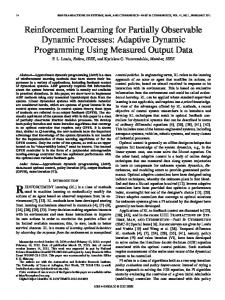
Fig. 1.
Learning phases.
example policy as a result of the interaction with the real environment. This paper is structured as follows. In Section II the learning procedure and the policy gradient algorithm are detailed. Section III describes all the elements that affect our problem: the underwater robot, the vision system, the simulated model and the controller. Details and results of the simulation process and the real test are given in Section IV and finally, conclusions and the future work to be done are included in Section V.
policy that converges to an optimal by computing approximations of the gradient of the averaged reward from a single path of a controlled POMDP. The convergence of the method is proven with probability 1, and one of the most attractive features is that it can be implemented online. In previous work [18], the same algorithm was used in a simulation task achieving good results. The procedure is summarized in Algorithm 1. The algorithm works as follows: having initialized the parameters vector θ0 , the initial state i0 and the eligibility trace z0 = 0, the learning procedure will be iterated T times. At every iteration, the parameters’ eligibility zt will be updated according to the policy gradient approximation. The discount factor β ∈ [0, 1) increases or decreases the agent’s memory of past actions. The immediate reward received r(it+1 ), and the learning rate α allows us to finally compute the new vector of parameters θt+1 . The current policy is directly modified by the new parameters becoming a new policy to be followed by the next iteration, getting closer to a final policy that represents a correct solution of the problem. Algorithm 1: Baxter and Bartlett’s OLPOMDP algorithm 1. Initialize: T >0 Initial parameter values θ0 ∈ RK Initial state i0 2. Set z0 = 0 (z0 ∈ RK ) 3. f or t = 0 to T do: (a) Observe state yt (b) Generate control action ut according to current policy µ(θ, yt ) (c) Observe the reward obtained r(it+1 ) ∇µ (θ,y ) (d) Set zt+1 = βzt + µ ut(θ,y t) t ut (e) Set θt+1 = θt + αt r(it+1 )zt+1 4. end f or
II. LEARNING PROCEDURES The introduction of prior knowledge in a gradient descent methodology can dramatically decrease the convergence time of the algorithm. This advantage is even more important when dealing with real systems, where timing is a key factor. Such learning systems divide its procedure into two phases or steps as shown in Fig. 1. In the first phase of learning (see Fig. 1(a)) the robot is being controlled by a supply policy while performing the task; during this phase, the agent extracts all useful information. In a second step, once it is considered that the agent has enough knowledge to build a “secure” policy, it takes control of the robot and the learning process continues, see Fig. 1(b). The proposal presented here takes advantage of learning by simulation as an initial startup for the learner. The objective is to transfer an initial policy, learned in a simulated environment, to a real robot and test the behavior of the learned policy in real conditions. First, the learning task will be performed in simulation with the aim of a model of the robot. Once the learning process is considered to be finished, the policy will be transferred to ICT IN EU AU V in order to test it in the real world. In a future task, the learning procedure will switch to a second phase, continuing to improve the policy while in real conditions. The Baxter and Bartlett approach [17] is the gradient descent method selected to carry out the simulated learning corresponding to phase one. The next subsection gives details about the algorithm. A. The gradient descent algorithm The Baxter and Bartlett’s algorithm is a policy search methodology with the aim of obtaining a parameterized
The algorithm is designed to work on-line. The function approximator adopted to define our policy is an artificial neural network (ANN) whose weights represent the policy parameters to be updated at every iteration step (see Fig. 2). As input, the network receives an observation of the state and, as output, a soft-max distribution evaluates each possible future state exponentiating the real-valued ANN outputs {o1 , ..., on }, being n the number of neurons of the output layer [4]. After applying the soft-max function, the outputs of the neural network give a weighting ξj ∈ (0, 1) to each of the possible control actions. The probability of the ith control action is then given by: exp(oi ) P ri = Pn a=1 exp(oa )
(1)
where n is the number of neurons at the output layer. Actions have been labeled with the associated control action and chosen at random from this probability distribution, driving the learner to a new state with its associated reward. Once the action has been selected, the error at the output layer is used to compute the local gradients of the rest of the network. The whole expression is implemented similarly
3636
Authorized licensed use limited to: UNIVERSITAT DE GIRONA. Downloaded on May 8, 2009 at 07:10 from IEEE Xplore. Restrictions apply.
to error back propagation [19]. The old network parameters are updated following expression 3.(e) of Algorithm 1: θt+1 = θt + αr(it+1 )zt+1
(2)
The vector of parameters θt represents the network weights to be updated, r(it+1 ) is the reward given to the learner at every time step, zt+1 describes the estimated gradients mentioned before and, at last, we have α as the learning rate of the algorithm. III. CASE TO STUDY: CABLE TRACKING This section is going to describe the different elements that take place into our problem: first, a brief description of the underwater robot ICT IN EU AU V and its model used in simulation is given. The section will also present the problem of underwater cable tracking and, finally, a description of the neural-network controller designed for both, the simulation and the real phases is detailed. A. ICT IN EU AU V
o1 State Input
on
Fig. 2.
Soft-Max
The underwater vehicle ICT IN EU AU V was originally designed to compete in the SAUC-E competition that took place in London during the summer of 2006 [20]. Since then, the robot has been used as a research platform for different underwater inspection projects which include dams, harbors, shallow waters and cable/pipeline inspection. The main design principle of ICT IN EU AU V was to adopt a cheap structure simple to maintain and upgrade. For these reasons, the robot has been designed as an open frame vehicle. With a weight of 52 Kg, the robot has a complete sensor suite including an imaging sonar, a DVL, a compass, a pressure gauge, a temperature sensor, a DGPS unit and two cameras: a color one facing forward direction and a B/W camera with downward orientation. Hardware and batteries are enclosed into two cylindrical hulls designed to withstand pressures of 11 atmospheres. The weight is mainly located at the bottom of the vehicle, ensuring the stability in both pitch and roll degrees of freedom. Its five thrusters will allow ICT IN EU AU V to be operated in the remaining degrees of freedom (surge, sway, heave and yaw) achieving maximum speeds of 3 knots (see Fig. 3).
Schema of the ANN architecture adopted.
ξ1
Fig. 3.
The autonomous underwater vehicle ICT IN EU AU V .
The mathematical model of ICT IN EU AU V used during the simulated learning phase has been obtained by means of parameter identification methods [21]. The whole model has been uncoupled and reduced to emulate a robot with only two degrees of freedom (DOF), X movement and rotation respect Z axis. B. The Cable Tracking Vision System The downward-looking B/W camera installed on ICT IN EU AU V will be used for the vision algorithm to track the cable. It provides a large underwater field of view (about 57◦ in width by 43◦ in height). This kind of sensor will not provide us with absolute localization information but will give us relative data about position and orientation of the cable with respect to our vehicle: if we are too close/far or if we should move to the left/right in order to center the object in our image. The vision-based algorithm used to locate the cable was first proposed in [22] and later improved in [23]. It exploits the fact that artificial objects present in natural environments usually have distinguishing features; in the case of the cable, given its rigidity and shape, strong alignments can be expected near its sides. The algorithm will evaluate the polar coordinates ρ (orthogonal distance from the origin of the camera coordinate frame) and Θ (angle between ρ and X axis of the camera coordinate frame) of the straight line corresponding to the detected cable in the image plane (see Fig. 4). Once the cable has been located and the polar coordinates of the corresponding line obtained, as the cable is not a thin line but a large rectangle, we will also compute the cartesian coordinates (xg ,yg ) (see Fig. 4) of the cable’s centroid with respect to the image plane by means of (3). ρ = xcos(Θ) + ysin(Θ)
(3)
ξn where x and y correspond to the position of any point of the line in the image plane. The computed parameters Θ, xg and yg together with its derivatives will conform the input of the neural-network controller (see Fig. 5). For the simulated phase, a downward-looking camera model has been used to emulate the vision system of the vehicle.
3637
Authorized licensed use limited to: UNIVERSITAT DE GIRONA. Downloaded on May 8, 2009 at 07:10 from IEEE Xplore. Restrictions apply.
C. The neural-network controller A one-hidden-layer neural-network with 6 input nodes, 3 hidden nodes and 5 output nodes was used to generate a stochastic policy. As can be seen in Fig. 5 the inputs to the network correspond to the normalized state vector comδxg δyg puted in the previous section s = {θ, xg , yg , δθ δt , δt , δt }. Each hidden and output layer has the usual additional bias term. The activation function used for the neurons of the hidden layer is the hyperbolic tangent type, while the output layer nodes are linear. The five output neurons represent the possible five control actions (see Fig. 6). The discrete action set A = {a1 , a2 , a3 , a4 , a5 } has been considered where A1 = (Surge, Y aw),A2 = (Surge, −Y aw),A3 = (−Surge, Y aw),A4 = (−Surge, −Y aw),A5 = (Surge, 0). Each action corresponds to a combination of a constant scalar value of Surge force (X movement) and Y aw force (rotation respect Z axis). As explained in Section II-A, the outputs have been exponentiated and normalized to produce a probability distribution. Control actions are selected at random from this distribution. IV. RESULTS A. 1srt phase: Simulated Learning The model of the underwater robot ICT IN EU AU V navigates a two dimensional world at 1 meter height above the seafloor. The simulated cable is placed at the bottom in a fixed circular position. The controller has been trained in an episodic task. An episode ends either every 15 seconds (150 iterations) or when the robot misses the cable in the image plane, whatever comes first. When the episode ends, the robot
Fig. 4.
Fig. 5.
The ANN used by the controller.
position is reset to a random position and orientation around the cable’s location, assuring any location of the cable within the image plane at the beginning of each episode. According to the values of the state parameters {θ, xg , yg }, a scalar immediate reward is given each iteration step. Three values were used: -10, -1 and 0. In order to maintain the cable centered in the image plane, the positive reward r = 0 is given when the position of the centroid (xg , yg ) is around the center of the image (xg ± 0.15, yg ± 0.15) and the angle θ is close to 90◦ (90◦ ± 15◦ ), a r = −1 is given in any other location within the image plane. The reward value of -10 is given when the vehicles misses the target and the episode ends. The number of episodes to be done has been set to 2000. For every episode, the total amount of reward perceived is calculated. Figure 7 represents the performance of the neuralnetwork robot controller as a function of the number of episodes when trained using Baxter and Bartlett’s algorithm on the controller detailed in Section III-C. The experiment has been repeated in 100 independent runs, and the results here presented are a mean over these runs. The learning rate
Coordinates of the target cable with respect ICT IN EU AU V .
Fig. 6.
ICT IN EU AU V discrete action set.
3638
Authorized licensed use limited to: UNIVERSITAT DE GIRONA. Downloaded on May 8, 2009 at 07:10 from IEEE Xplore. Restrictions apply.
Total R per Trial (mean of 100 rep.)
in Fig. 10 where the detected cable is shown while the vehicle performs a test inside the pool. Fig. 11 represents real measured trajectories of the θ angle while the vehicle performs different attempts to center the cable in the image. Finally, a short video is also provided where the vehicle uses the simulated policy to perform a real autonomous underwater cable tracking task.
0 -20
Mean Total R per Trial
-40 -60 -80 -100 -120
V. CONCLUSIONS AND FUTURE WORK
-140 -160
learning rate 0.001 discount factor 0.98
-180 -200 0
500
1000
1500
2000
Number of Trials
Fig. 7. Performance of the neural-network robot controller as a function of the number of episodes. Performance estimates were generated by simulating 2000 episodes. Process repeated in 100 independent runs. The results are a mean of these runs. Fixed α = 0.001, and β = 0.98.
was set to α = 0.001 and the discount factor β = 0.98. In Figure 8 we can observe a state/action mapping of a trained δxg δyg controller, yg and the state derivatives δθ δt , δt , δt have been fixed in order to represent a comprehensive graph. Figure 9 represents the trajectory of a trained robot controller. State-Action Mapping Representation, Centroid Y and derivatives fixed 4
5
3.5 4.3
3 3.6
350
This paper proposes a field application of a high-level Reinforcement Learning (RL) control system for solving the action selection problem of an autonomous robot in cable tracking task. The learning system is characterized by using a direct policy search algorithm for robot control based on Baxter and Bartlett’s direct-gradient algorithm. The policy is represented by a neural network whose weights are the policy parameters. In order to speed up the process, the learning phase has been carried out in a simulated environment and then transferred and tested successfully on the real robot ICT IN EU AU V . Results of this work show a good performance of the learned policy. Convergence times of the simulation process were not too long if we take into account the reduced dimensions of the ANN used in the simulation. Although it is not a hard task to learn in simulation, continuing the learning autonomously in a real situation represents a challenge due to the nature of underwater environments. Future steps are focused on improving the initial policy by means of on-line learning processes and comparing the results obtained with human pilots tracking trajectories.
2.5 3 300 250
-1.5 -1.5 200
2 2.3
-1 -0.5
150 0
1.5 1.6
100 0.5
Centroid X Position (Pixels)
50
1 0
Thetaangle angle (Radians) (Radiants) Theta
1
1
1.5
Fig. 8. Centroid X - Theta mapping of a trained robot controller. The rest of the state variables have been fixed. Colorbar on the right represents the actions taken.
B. 2nd phase: Learned policy transfer. Real test Once the learning process is considered to be finished, the weights of the trained ANN representing the policy are transferred to ICT IN EU AU V and its performance tested in a real environment. The robot’s controller is the same one used in simulation. The experimental setup can be seen
Fig. 9. Behavior of a trained robot controller, results of the simulated cable tracking task after learning period is completed.
3639
Authorized licensed use limited to: UNIVERSITAT DE GIRONA. Downloaded on May 8, 2009 at 07:10 from IEEE Xplore. Restrictions apply.
Fig. 10. ICT IN EU AU V in the test pool. Small bottom-right image: Detected cable.
VI. ACKNOWLEDGMENTS This work has been financed by the Spanish Government Comission MCYT, project number DPI2005-09001C03-01, also partially funded by the MOMARNET EU project MRTN-CT-2004-505026 and the European Research Training Network on Key Technologies for Intervention Autonomous Underwater Vehicles FREESUBNET, contract number MRTN-CT-2006-036186. R EFERENCES [1] R. Sutton and A. Barto, Reinforcement Learning, an introduction. MIT Press, 1998. [2] R. Sutton, D. McAllester, S. Singh, and Y. Mansour, “Policy gradient methods for reinforcement learning with function approximation,” Advances in Neural Information Processing Systems, vol. 12, pp. 1057–1063, 2000. [3] C. Anderson, “Approximating a policy can be easier than approximating a value function,” University of Colorado State,” Computer Science Technical Report, 2000.
Real Variation of the Theta angle while attempting to center the cable 1.6
1.5
Theta angle (Radiants)
1.4
1.3
1.2
1.1
1
0.9
0.8
0
20
40
60
80
100
120
140
160
180
[4] D. A. Aberdeen, “Policy-gradient algorithms for partially observable markov decision processes,” Ph.D. dissertation, Australian National University, April 2003. [5] J. Bagnell and J. Schneider, “Autonomous helicopter control using reinforcement learning policy search methods,” in Proceedings of the IEEE International Conference on Robotics and Automation, Korea, 2001. [6] M. Rosenstein and A. Barto, “Robot weightlifting by direct policy search,” in Proceedings of the International Joint Conference on Artificial Intelligence, 2001. [7] N. Kohl and P. Stone, “Policy gradient reinforcement learning for fast quadrupedal locomotion,” in IEEE International Conference on Robotics and Automation (ICRA), 2004. [8] P. Marbach and J. N. Tsitsiklis, “Gradient-based optimization of Markov reward processes: Practical variants,” Center for Communications Systems Research, University of Cambridge, Tech. Rep., March 2000. [9] V. Konda and J. Tsitsiklis, “On actor-critic algorithms,” SIAM Journal on Control and Optimization, vol. 42, number 4, pp. 1143–1166, 2003. [10] N. Meuleau, L. Peshkin, and K. Kim, “Exploration in gradient based reinforcement learning,” Massachusetts Institute of Technology, AI Memo 2001-003, Tech. Rep., April 2001. [11] R. Tedrake, T. W. Zhang, and H. S. Seung, “Stochastic policy gradient reinforcement learning on a simple 3D biped,” in IEEE/RSJ International Conference on Intelligent Robots and Systems IROS’04, Sendai, Japan, September 28 - October 2 2004. [12] T. Matsubara, J. Morimoto, J. Nakanishi, M. Sato, and K. Doya, “Learning sensory feedback to CPG with policy gradient for biped locomotion,” in Proceedings of the International Conference on Robotics and Automation ICRA, Barcelona, Spain, April 2005. [13] L. Lin, “Self-improving reactive agents based on reinforcement learning, planning and teaching.” Machine Learning, vol. 8(3/4), pp. 293– 321, 1992. [14] W. Smart, “Making reinforcement learning work on real robots,” Ph.D. dissertation, Department of Computer Science at Brown University, Rhode Island, May 2002. [15] C. Atkenson, A. Moore, and S. Schaal, “Locally weighted learning,” Artificial Intelligence Review, vol. 11, pp. 11–73, 1997. [16] B. Hammer, S. Singh, and S. Scherer, “Learning obstacle avoidance parameters from operator behavior,” Journal of Field Robotics, Special Issue on Machine Learning Based Robotics in Unstructured Environments, vol. 23 (11/12), December 2006. [17] J. Baxter and P. Bartlett, “Direct gradient-based reinforcement learning: I. gradient estimation algorithms,” Australian National University, Tech. Rep., 1999. [18] A. El-Fakdi, M. Carreras, and P. Ridao, “Towards direct policy search reinforcement learning for robot control,” in IEEE/RSJ International Conference on Intelligent Robots and Systems, 2006. [19] S. Haykin, Neural Networks, a comprehensive foundation, 2nd ed. Prentice Hall, 1999. [20] D. Ribas, N. Palomeras, P. Ridao, M. Carreras, and E. Hernandez, “Ictineu auv wins the first sauc-e competition,” in IEEE International Conference on Robotics and Automation, 2007. [21] P. Ridao, A. Tiano, A. El-Fakdi, M. Carreras, and A. Zirilli, “On the identification of non-linear models of unmanned underwater vehicles,” Control Engineering Practice, vol. 12, pp. 1483–1499, 2004. [22] A. Ortiz, M. Simo, and G. Oliver, “A vision system for an underwater cable tracker,” International Journal of Machine Vision and Applications, vol. 13 (3), pp. 129–140, 2002. [23] J. Antich and A. Ortiz, “Underwater cable tracking by visual feedback,” in First Iberian Conference on Pattern recognition and Image Analysis (IbPRIA, LNCS 2652), Port d’Andratx, Spain, 2003.
Number of Iterations
Fig. 11. Real measured trajectories of the θ angle of the image plane while attempting to center the cable.
3640
Authorized licensed use limited to: UNIVERSITAT DE GIRONA. Downloaded on May 8, 2009 at 07:10 from IEEE Xplore. Restrictions apply.