Reinforcement learning based dual-control ... - Semantic Scholar

IEEE TRANSACTIONS ON NEURAL NETWORKS, VOL. 19, NO. 8, AUGUST 2008

1369

Reinforcement-Learning-Based Dual-Control Methodology for Complex Nonlinear Discrete-Time Systems With Application to Spark Engine EGR Operation Peter Shih, Brian C. Kaul, S. Jagannathan, Senior Member, IEEE, and James A. Drallmeier

Abstract—A novel reinforcement-learning-based dual-control methodology adaptive neural network (NN) controller is developed to deliver a desired tracking performance for a class of complex feedback nonlinear discrete-time systems, which consists of a second-order nonlinear discrete-time system in nonstrict feedback form and an affine nonlinear discrete-time system, in the presence of bounded and unknown disturbances. For example, the exhaust gas recirculation (EGR) operation of a spark ignition (SI) engine is modeled by using such a complex nonlinear discrete-time system. A dual-controller approach is undertaken where primary adaptive critic NN controller is designed for the nonstrict feedback nonlinear discrete-time system whereas the secondary one for the affine nonlinear discrete-time system but the controllers together offer the desired performance. The primary adaptive critic NN controller includes an NN observer for estimating the states and output, an NN critic, and two action NNs for generating virtual control and actual control inputs for the nonstrict feedback nonlinear discrete-time system, whereas an additional critic NN and an action NN are included for the affine nonlinear discrete-time system by assuming the state availability. All NN weights adapt online towards minimization of a certain performance index, utilizing gradient–descent-based rule. Using Lyapunov theory, the uniformly ultimate boundedness (UUB) of the closed-loop tracking error, weight estimates, and observer estimates are shown. The adaptive critic NN controller performance is evaluated on an SI engine operating with high EGR levels where the controller objective is to reduce cyclic dispersion in heat release while minimizing fuel intake. Simulation and experimental results indicate that engine out emissions drop significantly at 20% EGR due to reduction in dispersion in heat release thus verifying the dual-control approach.

Index Terms—Adaptive critic design, near-optimal control, nonstrict feedback nonlinear discrete-time system, output feedback control, separation principle.

Manuscript received February 21, 2007; revised September 3, 2007 and December 29, 2007; accepted February 6, 2008. First published July 15, 2008; last published August 6, 2008 (projected). This work was supported by the National Science Foundation under Grants ECCS#0327877, and ECCS#0621924 and by the Intelligent Systems Center. P. Shih and S. Jagannathan are with the Department of Electrical and Computer Engineering, University of Science and Technology (formerly University of Missouri-Rolla), Rolla, MO 65409 USA (e-mail: [email protected]). B. C. Kaul and J. A. Drallmeier are with the Department of Mechanical and Aerospace Engineering, University of Science and Technology (formerly University of Missouri-Rolla), Rolla, MO 65409 USA. Color versions of one or more of the figures in this paper are available online at http://ieeexplore.ieee.org. Digital Object Identifier 10.1109/TNN.2008.2000452

I. INTRODUCTION

A

DAPTIVE control using neural network (NN) in general is now well understood for affine nonlinear discrete-time systems. Additionally, backstepping control of nonlinear discrete-time systems in strict feedback form in particular has been addressed in the literature [1]–[3]. The strict feedback nonlinear discrete-time system is expressed as [1] (1) (2) where

is the state,

is the control input, , and . For strict feedback nonlinear systems [1], the nonlinearities and depend only upon , . However, for a nonstrict feedback nonlinear system, i.e., and depend on both and where , there were no control design schemes available until recently [11]. Since available [1]–[3] methods when applied to a second-order nonlinear nonstrict feedback discrete-time systems will result in a noncausal controller (current control input depends on the future system states), control design for nonstrict feedback systems should be handled carefully [11]. On the other hand, though stable NN controllers [1]–[3], [10]–[13] are designed for nonlinear discrete-time systems, these control designs fail to render optimality since tracking error was utilized as the performance measure. By contrast, the reinforcement-learning-based adaptive critic NN approach [4] has emerged as a promising tool to develop optimal (or suboptimal) NN controllers due to its potential to find approximate solutions to dynamic programming, where a strategic utility function, which is considered as the long-term system performance measure, can be optimized. Optimal NN controllers using reinforcement learning are considered as the third generation NN controllers and they are currently being pursued by many researchers [4]–[9], [15], [19], [21]. In supervised learning, an explicit signal is provided by the teacher to guide the learning process whereas in the case of reinforcement learning, the role of the teacher is more evaluative than instructional in nature. The critic NN monitors the system states and approximates the strategic utility function, and provides a better training signal to the action NN, which generates the near-optimal control action to the nonlinear system.

1045-9227/$25.00 © 2008 IEEE Authorized licensed use limited to: University of Missouri. Downloaded on December 18, 2008 at 11:59 from IEEE Xplore. Restrictions apply.

1370


There are many variants of adaptive critic NN controller architectures [4]–[9] using state feedback even though few results [6]–[9], [19] address the controller convergence. However, adaptive critic NN controller results were not available for the nonlinear discrete-time systems in nonstrict feedback form until recently [22]. By contrast, in [18], a novel NN controller using tracking error as the performance measure is introduced for nonlinear discrete-time systems in nonstrict feedback form. To the best of our knowledge, no known results are available for near-optimal control of complex nonlinear discrete-time systems using reinforcement learning such as the ones introduced in this paper. In this paper, a novel adaptive critic NN-based feedback controller is developed to control a class of complex nonlinear discrete-time systems, which consists of a coupled nonstrict feedback plus an affine system, with bounded and unknown disturbances. A dual-control approach is undertaken where a primary adaptive critic NN controller is designed for nonlinear discrete-time systems in nonstrict feedback form and a secondary controller for the affine nonlinear discrete-time systems so that both controllers work together guaranteeing performance and stability. For the case of a nonlinear discrete-time system in nonstrict feedback form, an adaptive NN backstepping is utilized for the controller design with two action NNs being used to generate the virtual and actual control inputs, respectively. The weights of the two action NNs are tuned by the critic NN signal to minimize the strategic utility function and their outputs. The critic NN approximates certain strategic utility function a variant of standard Bellman equation. The NN observer estimates the system states and output and the estimates are subsequently used in the controller. The proposed controller is model-free since the dynamics of the nonlinear discrete-time systems are not known beforehand. All the NN weights are tuned online. On the other hand, for the affine nonlinear discrete-time system, a separate critic and action NNs are utilized. The critic NN approximates the standard Bellmann equation and tunes the action NN so that the action NN generates a near-optimal signal to control the affine nonlinear discrete-time system. Both controllers work together and render guaranteed performance and closed-loop stability. The main contributions of this paper can be summarized as follows. 1) The adaptive critic NN approach is extended to a complex nonlinear discrete-time system where a dual-control approach is undertaken while guaranteeing stability and performance. 2) Optimization of a long-term performance index is undertaken in contrast with traditional adaptive NN schemes [1], [2] where no optimization is performed. 3) Demonstration of the boundedness of the overall system is shown even in the presence of NN approximation errors and bounded unknown disturbances unlike in the existing adaptive critic design (ACD) works [7]–[9] where the convergence is presented under ideal circumstances. Stability proof is inferred even with an NN observer by relaxing the separation principle via novel weight-updating rules and by selecting the Lyapunov function consisting of the system

estimation errors, tracking, and the NN weight estimation errors. A single critic NN is utilized to tune two action NNs. 4) A well-defined controller is presented by overcoming the problem of certain nonlinear function estimates becoming zero since a single NN is used to approximate both nonlinear functions and compared to [10]. 5) The NN weights are tuned online instead of offline [5]. is bounded away 6) The assumption that from zero and its sign is known a priori is relaxed in contrast with [2]. The proposed primary controller is applied to control the spark ignition (SI) engine dynamics operating with high exhaust gas recirculation (EGR) levels, a practical complex nonlinear discrete-time system. The primary controller allows the engine, which is a nonstrict feedback nonlinear discrete-time system to operate in high EGR mode with fuel intake as the control input, where an inert gas displaces the stoichiometric ratio of fuel to air. The inert gas system is modeled as an affine nonlinear discrete-time system, and therefore, a separate secondary controller is designed. Both controllers enable the engine to operate in higher EGR mode compared to the uncontrolled case by reducing heat release dispersion while minimizing fuel intake. Consequently, the engine exhibits improved emissions and fuel efficiency compared to the uncontrolled case. Other controller designs can run an SI engine in lean mode [11]; however, engine catalysts cannot function efficiently with the lean exhaust chemistry. EGR, on the other hand, allows for the efficient operation of standard three-way catalysts. Not only does it reduce precatalyst emissions, but it can improve fuel efficiency by reducing throttling losses. Therefore, the applicability of high EGR usage in the automotive engines is greater. Dilution with EGR also has wide practical applicability in diesel engines and in SI engines without three-way catalysts. II. COMPLEX NONLINEAR DISCRETE-TIME SYSTEMS Consider the complex nonlinear discrete-time system, given in the following form:

(3) (4) (5) (6) , , are states, and where are system inputs, and , , and are unknown but bounded disturbances. Bounds on the dis, , and turbances are given by where , , and are unknown positive scalars. It is important to note that the output is a nonlinear function of states in contrast with available literature [12], [13] where the output is a linear function of the states. Finally, the output is considered measurable whereas the first two states

Authorized licensed use limited to: University of Missouri. Downloaded on December 18, 2008 at 11:59 from IEEE Xplore. Restrictions apply.

SHIH et al.: REINFORCEMENT-LEARNING-BASED DUAL-CONTROL METHODOLOGY

and are considered not available while is assumed to be available for convenience. For the systems (3) and (4), not only should the systems’ actual output converge to their target value, but the states should also converge to their respective desired values for the proposed application of engine control. The controller development is presented separately for the two systems as the objectives are different even though the two controllers are designed for the same complex system. The first part uses (3), (4), and (6) to develop the primary controller. The second part uses (5) to develop the secondary controller. Stability for both systems is demonstrated together. The SI engine control with high levels is represented by (3)–(6), and therefore, the class of systems is of interest. One cannot directly apply the controller design from nonstrict feedback nonlinear discrete-time systems [11], [18] since the first system contains the third state unlike a typical nonstrict feedback system. Therefore, a dual approach is the best choice.

1371

represents the hidden layer activation control input, is the number of nodes in the hidden layer, and function, is the approximation error. For simplicity, the two equations can be represented as (12) and (13) Rewrite (11) using (12) and (13) to obtain (14) The states and are not measurable; therefore, is not available either. Using the estimated and measured , and , respecstates and the output, tively, instead of , , and , the proposed observer is given as

III. PRIMARY CONTROLLER To overcome the immeasurable states and , an , observer is used. It utilizes the current heat release output, and states to estimate the future output and . The design of the observer, which follows steps similar to [22] is discussed next. A. Observer Design For the observer design, the nominal values of the uncertainties are required since the nonlinearities as well as the input–output relationship is considered unknown. The nominal values of the unknown uncertainties can be obtained by a variety of ways. One of the ways is to apply Taylor series expansion without ignoring the higher order terms. Consider (3) and (4). We expand the individual nonlinear functions using Taylor series expansion into linear and higher order terms (7) (8)

(15) is the where and are the esinput vector using estimated states, timated future and the current output, is the actual weight matrix, is the estimated control input, is the hidden layer activation function, is the observer gain, and is the heat release estimation error defined as (16) It is demonstrated in [14] that, if the hidden layer weights are chosen initially at random and kept constant, and the number of hidden layer nodes is sufficiently large, then the approximacan be made arbitrarily small so that the tion error holds for all since the bound activation function forms a basis to the nonlinear function that the NN approximates. Now we choose, at our convenience, the observer structure as a function of output estimation errors and known quantities as

(9) (10) where the first term in (7)–(10) are known nominal values and the second term are unknown higher order terms. The entire expansion for the terms in (7)–(10) is not necessary since it is not required for the controller design. Moreover, the higher order terms are not ignored. A two-layer feedforward NN with semirecurrent architecture and novel weight tuning are utilized to construct the output as (11)

(17) (18) and are design constants. where Define the state estimation and output errors as (19) (20) Combining (17)–(20), to obtain the estimation and output error dynamics as

is the where and are the future and current network input, and denote the ideal output and outputs, constant hidden layer weight matrices, respectively, is the Authorized licensed use limited to: University of Missouri. Downloaded on December 18, 2008 at 11:59 from IEEE Xplore. Restrictions apply.

(21) (22)

1372


and

B. Reinforcement Learning and Optimization

choose the weight tuning of the observer as

The purpose of the critic NN is to approximate the long-term performance index (or strategic utility function) of the nonlinear system through online weight adaptation. The critic signal estimates the future performance and tunes the two action NNs. The tuning will ultimately minimize the strategic utility function itself and the action NN outputs or control inputs to the system so that closed-loop stability is inferred. is given by The utility function

(23)

(24) where and are design constants. It will be shown in Section III-D that by using the above weight tuning, the separation principle is relaxed and the closed-loop signals will be bounded. Next, we present the theorem, where it is demonstrated that the state estimation and output estimation errors along with observer NN weight estimation errors are bounded. The following mild assumptions are required. Assumption 1: The unknown smooth functions and are upper bounded within the compact set as and . Remark: This assumption is a direct consequence of functions over the compact sets. This assumption is required for the NN universal approximation result to hold. Theorem 1 (Observer Stability): Consider the system given by (3), (4), and (6), and the disturbance bounded by and where and are known positive scalars. Let the observer NN weight tuning be given by (24). The and , output estimation errors state estimation errors , and NN weight estimate of the observer are uniformly ultimate boundedness (UUB), with the bounds specifically given by (B.11), with the controller design parameters selected as (25)

if otherwise

(30)

is a user-defined threshold. The utility function where represents the current performance index. In other words, and refer to good and unsatisfactory tracking performance at the th time step, respectively. The long-term is defined as strategic utility function

(31) , , is the discount factor and is the where is viewed here as the long system horizon index. The term performance measure for the controller since it is the sum of all future system performance indices. Equation (31) can also after be expressed as simple manipulation, which is similar to the standard Bellman equation. C. Critic NN Design We utilize the universal approximation property of NN to define the critic NN output and rewrite as

(26)

(32)

(27)

where is the critic signal, is the tunable weight matrix, represents the constant input weight matrix selected initially at random, is the activation function vector in the hidden is the number of the nodes in the hidden layer, and layer, is the input vector. We define the prediction error as

(28) (29) is the NN adaptation gain and , , , and are the where observer design parameters. Proof: Follow steps similar to [22]. See Appendix B for the proof. Remark 1: In Theorem 1, state and output estimation errors and the NN weights of the observer are shown to be bounded. One can then design a controller by applying separation principle if the system under consideration is linear. Unfortunately, separation principle does not hold for nonlinear systems. Therefore, in Section III-D, the boundedness of the closed-loop system is demonstrated where the observer and controller signals are proven to be bounded without using separation principle. Next we discuss the design of the adaptive critic NN controller for the primary system and demonstrate that if the closed-loop system is bounded then the control inputs will be bounded.

(33) where the subscript “ ” stands for the “critic.” We use a quadratic objective function to minimize (34) The weight-update rule for the critic NN is based upon gradient adaptation, which is given by the general formula (35) where


(36)


or

(37) where

is the NN adaptation gain.

D. Action NN Design In this section, the design of the virtual control input is discussed. Before we proceed, the following mild assumption is needed. Then, the system of nonlinear equations is rewritten. is Assumption 2: The unknown smooth function and within the bounded away from zero for all , compact set . In other words, , and , where and . is positive Without loss of generality, we will assume that in this paper. First, we simplify by rewriting the state equations with the following: (38)

1373

chosen initially at random and kept constant, and the number of hidden layer nodes is sufficiently large, then the approximation can be made arbitrarily small so that the bound error holds for all in a compact set, since the activation function vector forms a basis to the nonlinear function that the NN approximates. Rewriting (43) using (44), the virtual control signal can be rewritten as (45) Replacing actual with estimated states, (45) becomes

(46) where using estimated states, and Define

is the input vector . (47)

Equation (42) can be rewritten using (47) as

Systems (3) and (4) can be rewritten as (39) (40) 1) Virtual Control Input Design: Our goal is to stabilize the around a specified target point by consystem output aptrolling the input. The secondary objective is to make proach the desired trajectory . At the same time, all signals in systems (3) and (4) must be UUB, all weights must be bounded, and a performance index must be minimized. Define the tracking error as

(48) Combine (46) into (48), then (44) to get

(41) where is the desired trajectory. Using (39), (41) can be expressed as the following:

(42) By viewing as a virtual control input, a desired virtual control signal can be designed as (49)

(43) where

is a gain constant. Since is an unknown function, in (43) cannot be implemented in practice. We invoke the universal approximation property of NN to estimate this unknown function

where (50) and (51)

(44) where

is the input vector, and are the ideal and constant input is the activation function weight matrices, is the number of the nodes in the vector in the hidden layer, is the functional estimation error. It hidden layer, and is demonstrated in [14] that, if the hidden layer weights are

Let us define (52) is defined in (32), and the where the error for the first action NN,


subscript represents . The desired

1374


strategic utility function is “0” to indicate perfect tracking at all steps. Thus, (52) becomes

weights constant and adapt the output weights only. We also replace actual with estimated states to design the control input as

(53) (60) The objective function to be minimized by the first action NN is given by (54)

where , is the input vector. Rewriting (47) and substituting (58)–(60), we get

The weight-update rule for the action NN is also a gradientbased adaptation, which is defined as (55) where (56) (57) with is the NN adaptation gain. 2) Actual Control Design: Choose the following desired control input:

(61) where (62)

(58) is noncausal since it depends upon future value Note that . We solve this problem by using a semirecurrent of NN since it can be a one-step predictor. The term depends on state , virtual control input , desired tra, and system errors and . By taking jectory can the independent variables as the input to an NN, be approximated during control input selection. Consequently, in this paper, a feedforward NN with properly chosen weight tuning law rendering a semirecurrent or dynamic NN can be used to predict the future value. Alternatively, the value can be obtained by employing a filter [15]. The first layer of the second NN using the system errors, state estimates, and past as inputs generates , which in turn is value used by the second layer to generate a suitable control input. The results in the simulation section show that the overall controller performance is satisfactory. On the other hand, one can use a single-layer dynamic NN to generate the future value of , which can be utilized as an input to a third control NN to generate a suitable control input. Here, these two single-layer NNs are combined into a single-multilayer NN. Define input as , then can be approximated as

(59) and denote the constant ideal where is the acoutput and hidden layer weight matrices, tivation function vector, is the number of hidden-layer nodes, is the estimation error. Again, we hold the input and

and (63) Equations (49) and (61) represent the closed-loop error dynamics. Next we derive the weight-update law. Define (64) is the error and the subscript stands for where the second action NN. Following the similar design, choose a quadratic objective function to minimize (65) Define a gradient-based adaptation where the general form is given by (66) (67) or in other words (68) The proposed controller structure is shown in Fig. 1. Next, in Theorem 2, it is demonstrated that the closed-loop system is UUB. Before we proceed, the following assumptions are needed. Assumption 3 (Bounded Ideal Weights): Let , , , and be the unknown output layer target weights for the observer,



1375

Fig. 1. Combined primary and secondary controller structure.

critic, and two action NNs, and assume that they are bounded above so that

(75) (76)

(69)

(77)

where , , and represent the bounds on the unknown target weights, and where the Frobenius norm [15] is used. Fact 1: The activation functions are bounded above by known positive values so that

(78) (79) (80)

(70)

(81)

, , , where are the upper bounds. and Theorem 2 (Output Feedback Controller Stability): Consider the system given by (3) and (4) and the disturbance bounds and to be known constants. Let the observer, critic, virtual control, and control input NN weight tuning be given by (24), (37), (57), and (68), respectively. Let the virtual control input and control input be given by (46) and (60). The estimation erand and weight estimates rors and tracking errors , , , and are UUB, with the controller design parameters selected as

where , , , and are NN adaptation gains, , , , , , and are controller gains, and is employed to define the strategic utility function. Proof: Follow steps similar to [22]. Proof is presented in Appendix B with Theorem 4. Remark 2: A well-defined controller is developed in this paper since a single NN is utilized to approximate two nonlinear functions even though a second-order nonlinear nonstrict feedback discrete-time system is considered as the primary system. The causal problem encountered in the proposed work is due to the nonstrict feedback issue whereas the causal nature encountered in [23] is due to the th-order strict feedback system. In [23], it was shown how a suitable coordinate transformation can be utilized to overcome the causal problem. Similar approach can be found for the proposed nonstrict feedback nonlinear discrete-time system as well. However, extension to an th-order system is outside the scope of this work.

(71) (72) (73) (74)


1376


Remark 3: Generally, the separation principle used for linear systems does not hold for nonlinear systems, and hence it is relaxed in this paper for the controller design since the Lyapunov function is a quadratic function of system errors and weight estimation errors of the observer and controller NNs. Remark 4: It is important to note that in this theorem persistency of excitation condition (PE) condition for the NN observer and NN controller and the linearity in the parameters assumption are not needed, in contrast with standard work in the discrete-time adaptive control, since the first difference does not require the PE condition to prove the boundedness of the weights. Even though the input to the hidden-layer weight matrix is not updated and only the hidden- to the output-layer weight matrix is tuned, the NN method relaxes the linear in the unknown parameter assumption. Additionally, the certainty equivalence principle is not used. Remark 5: The NN weight tuning proposed in (24), (37), (57), and (68) renders a semirecurrent NN due to the proposed weight tuning law even though a feedforward NN is utilized. Here the NN outputs are not fed as delayed inputs to the network whereas the outputs of each layer are fed as delayed inputs to the same layer. This semirecurrent NN architecture renders a dynamic NN, which is capable of predicting the state one step ahead. Remark 6: The need for an exact model of the nonlinear discrete-time in many existing ACD approaches [5], [6] is relaxed in our work. The action NNs will learn the unknown system dynamics through the feedback signals from the closed loop so that it can generate a near-optimal control input. The proposed actor–critic architecture will render a model-free approach. Remark 7: It is important to note that the output-layer weights of the action and critic NN can be initialized at zero or random. This means that no explicit offline training phase is necessary and the updating of the NNs is performed in an online manner. This is in contrast with many ACD designs where some a priori training is needed. Additionally, the proposed methodology does not require stop/reset strategy utilized by certain adaptive critic schemes [6]. Remark 8: Compared to other adaptive critic or reinforcement learning schemes [5], [6], the proposed approach ensures closed-loop stability using the Lyapunov approach even though gradient-based adaptation is employed. Remark 9: It is only possible to show the boundedness of all the closed-loop signals by using an extension of Lyapunov stability [15] due to the presence of approximation errors and bounded disturbances consistent with the literature. Consequently, a near-optimal solution can be demonstrated by using the update laws of the critic and action NNs. Remark 10: Equations (71)–(80) relate to the selection of adaptation gains whereas (81) provides how the discount factor can be chosen in order to ensure stability and convergence. Such a relationship does not exist in the past adaptive critic literature where the discount factor and adaptation gains are selected by trail and error procedure. Remark 11: With the proposed approach, the learning can be performed simultaneously both in the critic and action NNs in contrast with some of the available schemes where the learning is first accomplished by the critic NN and then by the action NN.

Corollary 1: The proposed adaptive critic NN controller and the weight-updating rules with parameter selection based on (71)–(81) cause the state to approach the desired virtual control input . Proof: Combining (45) and (46), the difference between and is given by (82) is the first action NN weight estimation where error and is defined in (50). Since both and are bounded, is bounded near . In is bounded, i.e., the state Theorem 1, we show that is bounded to the virtual control signal . Thus, the state is bounded to the desired virtual control signal . IV. SECONDARY CONTROLLER DESIGN To simplify the controller development, the third equation can be simplified as (83) where . This equation can be represented as a standard affine nonlinear discrete-time system. The controller design for this system is different than the nonstrict feedback nonlinear discrete-time system given by (1) and (2). Therefore, the design of a novel reinforcement controller is introduced here by assuming that the third state is measurable. For maintaining dilution to a desired level, the third equation as the control input and inert gas will be employed with EGR as an additional state. It is important to notice that the residual gas fraction is not known in advance though upper bounded is known. The objective of the secondary controller is to force the to approach its target value error between the actual state . Define (84) A. Critic NN Design Let the long-term cost function be defined as (85) where (86) with and are positive definite matrices and is the discount selected by the designer. factor within the range of Invoke the universal approximation property of NN to estimate (85) as (87) is the estimation error. Replace the states with where estimated states (88) where and denote the ideal output and is the activation constant hidden-layer weights, is the number of hidden-layer nodes. function vector, and



Again, we hold the input weights constant and adapt the output as the weights only. Take input vector. Define the prediction error as

1377

Define the control input cost function

(99)

(89)

where is the desired long-term cost function and is equal to zero. Define a quadratic error to minimize

where

(100) (90)

Utilizing a gradient–decent minimization strategy

Using a quadratic minimizing function (91) Using a standard gradient-based adaptation method, the weight update is given by

(92)

The disturbance and the approximation errors are taken as zero for the sake of weight tuning. Then, action NN weight tuning for the secondary controller can be expressed as

The control design is described next. B. Action NN Design

(101)

The tracking error is defined as

(93) is the target bounded trajectory. Define the desired where control signal as (94) where is a design parameter. Using the universal approximation property of NN and the approximate states (95) and denote the ideal output- and where is the acticonstant hidden-layer weight matrices, is the number of hidden layer nodes, vation function vector, is the input vector. and Again, we hold the input weights constant and adapt the output weights only. Rewrite (93) as

(96) where (97) and (98)

The structure of the combined primary and secondary controller is shown in Fig. 1. Next the stability of the closed-loop system of the secondary controller is demonstrated. Before we proceed, the following mild assumptions are stated. and be the unknown output-layer Assumption 4: Let target weights for the action and critic NNs, respectively, and and assume that they are bounded such that where and represent the bounds on the ideal weights. Fact 2: The activation functions for the action and critic NNs of the secondary controller are bounded by known positive and , where values, such that denote the upper bound for the activation functions. is Assumption 5: The unknown smooth function within the bounded away from zero for all , compact set . In other words, , where and . Without loss of generality, we will assume is positive in this paper. Additionally, the NN approxthat and are bounded above in imation errors the compact set by and [15]. Remark 12: The tracking and weight estimation errors will be expressed as a function of NN approximation errors and bounded disturbances. Even if the Assumption 5 is assumed, unless the NN weight tuning is properly selected, the entire system will not be stable. in (97) is Fact 2: With the Assumption 4, the term by bounded over the compact set .


1378


Theorem 3 (Secondary Controller Stability): Consider the to secondary system given by (5) and the disturbance bound be known constants. Let the virtual and control input NN weight tuning be given by (92) and (101), respectively. Let the control and weight esinput be given by (95); the tracking error and are UUB with the controller design timates parameters selected as

(109) (110) (111)

(102) (103)

(112) (113) (114) (115)

(104) where and are NN adaptation gains and is the controller gain. Proof: Proof is combined with Theorem 4. Remark 13: Theorem 3 demonstrates the UUB of the secondary controller for the closed-loop system. The primary and secondary controller designs introduced here are analogous to dual-controller design approach in the literature [20]. Theorem 4 (Overall System Boundedness): Consider the , system given by (3)–(6) and the disturbance bounds , and to be known constants. Let the observer, critic, virtual control, and control input NN weight tuning be given by (24), (37), (57), and (68), respectively, for the primary adaptive controller whereas virtual and control input NN weight tuning be given by (92) and (101), respectively. Let the virtual control input and control input for the primary and secondary controllers be given by (46), (60), and (95), respectively, then the estimation and tracking errors and weight estimates , , , , , and are UUB with the bounds given in (B.35) provided the design parameters are selected as (71)–(81) and (102)–(104). Proof: See Appendix B. V. RESULTS AND ANALYSIS EGR operation of an SI engine allows lower emissions and improved fuel efficiency. However, EGR operation destabilizes the engine due to the cyclic dispersion of heat release. The adaptive critic NN controller is designed to stabilize the SI engine operating at EGR conditions.

, , and represent total mass of air, fuel, where is the heat and inert gas, respectively, of the engine and release at th time instant. The value of combustion efficiency is denoted by , which is bounded by with maximum combustion efficiency being unity. Residual gas fraction is bounded by , which is typically unknown. and are unknown but bounded disturbances bounded by and with and being unknown positive scalars. The terms , , and are equivalence ratio system parameters. The terms , , , and are the mass of water, oxygen, nitrogen, and carbon dioxide, respectively, whereas , , , , and are design constants, and constants associated with their respective chemicals. Equations (105) and (106) represent the second-order nonstrict feedback nonlinear discrete-time systems whereas (107) can be controlled by the secondary controller. In this paper, for convenience, we assume that the secondary controller provides a bounded value to the primary system by setting the EGR at discrete levels. We set it to a constant that will simplify the controller implementation, as the third state is considered to be a fixed value. Note that this deterministic model accounts for stochastic effects by randomly fluctuating parameters such as injected air-fuel ratio or residual fraction. Other complex processes like temperature variation, turbulence, and fuel vaporization are not modeled but are assumed to add additional noise to the engine output. To implement the observer, replace the following from the Daw model into the general case:

A. Daw Engine Model SI engine dynamics can be expressed according to the Daw model as a class of nonlinear systems in a nonstrict feedback form [16]. At high EGR levels, the engine can be expressed as a combination of nonstrict feedback nonlinear discrete-time systems plus affine nonlinear discrete-time system given by [17]

(116) and

(105) (106) (117) (107) (108)

, because they are Note that we omitted the residuals in not available. The error introduced by this is accounted for in



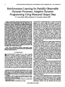
Fig. 2. Uncontrolled and controlled heat release return map at 13% EGR. Heat release at k

the air estimation error. To implement the controller, replace the and : following in place of

(118) To calculate the nominal values in (117), we run the engine at different EGR levels in an uncontrolled manner at the stoichiometric fuel to air ratio. That will give us the nominal fuel, air, , , and . From those, comand equivalence ratio— bustion efficiency is calculated. B. Simulation Results in conjunction The controller is easily simulated in with the Daw model. The learning rates for the observer (71), critic (72), virtual control input (73), and control input (74) networks and for the secondary controller are , and , respectaken as are selected as tively. The gains , , , , , , and , and . The system constants , , and are chosen as , and . The critic are and for both controllers for all constants and EGR levels. All NNs use 20 hidden neurons with hyperbolic tangent sigmoid activation functions in the hidden layer. The simulation parameters selected were as follows. An equivalence ratio of one was maintained with stochastic varifor iso-octane, residual gas fraction ation of 1%, , mass of nominal new air , mass of , the standard deviation of mass of nominal new fuel , cylinder volume in moles to match new fuel is , the experimental constraint, molecular weight of fuel , , , and molecular weight of air . EGR was assumed to be maximum combustion efficiency . an inert mixture with a molecular weight of The last two system variables, disturbances and stochastic effects, are modeled as follows. First, we assume a Gaussian distribution governs the two effects. We may inject disturbances to and , but a the two states in (105) and (106) due to simpler method is to perturb the equivalence ratio (109). This simplification is sufficient because the states are not measurable; therefore, the disturbances are increasingly complex and

1379

+ 1 instance is plotted against heat release at k instance.

immeasurable. Stochastic effects alter the output, and through the combustion efficiency (110) and finally the output (108), this single perturbation effectively models the last two system variables. The final model uses a Gaussian distribution noise injected into (109) centered around the target equivalence ratio . The resulting simulation output matches and deviation of to the output observed from the Ricardo engine. All simulations ran for uncontrolled 5000 cycles first, and then 5000 controlled cycles. Fig. 2 shows two heat release return maps, one controlled and the other uncontrolled, for the set point at 13% EGR. Each figure shows the next time step versus the current time step heat release. Points centered along the 45 line represent heat release values that are equal to the next step heat release. Note the clustering of the points around the mean heat release of 850 J. The square represents the target heat release. At this set point, the heat release dispersion starts to affect the engine performance, indicated by the stray points away from the central cluster. There are no complete misfires, but the heat release variation can be clearly seen. Fig. 3 shows the time series of the heat release and control input at the same EGR level. The controller activates after several thousand cycles, indicated by the fluctuation of the control output. The controller converges quickly and to a stable operation point. The presence of spikes in the control output indicates a decline in heat release such as a misfire, translating into additional fuel control to counteract. Figs. 4 and 5 depict another set point at 19% EGR. Similar features appear compared to the previous EGR level, except with higher frequency and amplitude of dispersion. Improvements shown reflect the assertion of the control action. In order to quantify the performance of the controller, we compare the coefficient of variation (COV), which is the standard deviation normalized by dividing the mean of the heat release. As the COV decreases, the standard deviation decreases, which indicates that the engine heat release is more stable compared to higher COV. The controller performs better, and the return map consequently should approach the target value. Table I tabulates all of the data from the simulation. The COV of each set point decreased drastically (shown with a negative sign) as the controller operated. The performance exceeded the improvement due to the slight increase in the mean fuel input. Next, we show that experimental data supports the simulation data.


1380


Fig. 3. Heat release versus iteration number at 13% EGR. Controller turns on at k = 4000. Note the almost instant learning convergence of the controller.

Fig. 4. Uncontrolled and controlled heat release return map at 19% EGR.

Fig. 5. Heat release and control input at 19% EGR.

C. Experimental Results Using Ricardo Engine The experimental results are collected from a Ricardo hydra engine with a modern four-valve Ford Zetek head. It contains a single cylinder running at 1000 r/min with shaft encoders to signal each crank angle degree and start of cycle. There are 720 per engine cycle. In the cylinder, a piezoelectric pressure transducer records pressure every crank angle degree. Combustion is considered

to take place between 345 and 490 , for a total of 145 pressure measurements. The cylinder pressure is integrated along with volume during the 17.7-ms calculation window. All communications are completed at this time. The output of our controller controls the fuel input. This is controlled by a transistor–transistor logic (TTL) signal to a fuel injector driver circuit. All signals communicate through a custom interface board using a microcontroller. The board interfaces with the PC



Fig. 6. Uncontrolled and controlled heat release return map at EGR

= 18%. Heat release at k + 1 instance is plotted against heat release at k instance.

Fig. 7. Uncontrolled and controlled heat release return map at EGR

= 18%. Heat release at k + 1 instance is plotted against heat release at k instance.

through a parallel port and with the engine hardware through an analog signal. All constants given in the simulation section are used in the experiment. The first operation for an engine run is to measure the air flow and nominal fuel. The desired EGR set point equation is given by

EGR

(119)

where is the mass of inert gas introduced at each cycle, which is nitrogen in the lab and exhaust gas in production applications and and are mass of fuel and mass of air, respectively. These values are loaded into the controller. Ambient pressure is used to reference the in-cylinder pressures when the exhaust valve is fully open and subtracted from the combustion pressure measurements. Uncontrolled and controlled data were collected at EGR percentages of 18, 20, and 23. The uncontrolled engine

1381

ran for 5000 cycles and then the controller is turned on for another 5000 cycles. Steady state was ensured prior to data collection by measuring stable exhaust temperatures. Fig. 6 shows two heat release return maps, one controlled and the other uncontrolled, for the 18% EGR set point. The target heat release is at 870 J. At this EGR level, cyclic dispersion can clearly be seen, indicated by deviation of the points away from the main cluster on the 45 line. Fig. 7 shows the time series of the heat release and control input for the same set point. Define the state and output tracking errors as

(120) where and are state 1 and state 2 tracking errors, respectively. Fig. 8 shows the controller state tracking errors at a set point of 18% EGR. The range represents tracking error in percentage over and under the desired state trajectories. State 1 tracking error is considerably better than state 2 tracking. The second state tracks within 0.5%; therefore, both are performing


1382


Fig. 8. State tracking errors.

TABLE I COV AND FUEL DATA FOR EACH OF THE FOUR SET POINTS

the target point. It is difficult to determine success on cycles with no misfire, because no heat release plots are available for uncontrolled case during the same cycles when the controller is operating for comparison. Overall, the controller performs to general expectation. Table II shows the improved COV when the controller is in operation compared to an uncontrolled engine along with the corresponding change in nominal fuel. At all EGR set points except 23%, the increase in fuel input is well within the tolerance of the equipment. On average, the COV decreases significantly by 25% compared to the uncontrolled case. For the 23% EGR, the drop is around 12%. The COV and fuel change data indicate an improved performance compared to the previous controller where a simple tracking error is utilized without any optimization criteria [18]. The average drop in COV was 17% between uncontrolled and controlled cases, compared to 25% for the current controller. Although this seems to indicate an increase in performance, we must also consider the increase in average fuel input in conjunction. The previous controller increased the average fuel to 2.4%, which is well beyond the detection error and significant in the engine application. This controller, however, averages less than 1%, safely below the detection error. The controller fuel increases negligibly while performing better than the previous controller due to the incorporation of the performance index. Therefore, this controller outperforms other NN controller and at the same time exerts less impact on the fuel.

VI. CONCLUSION well. The spikes indicate unsuccessful tracking. Consequently, the observer and controller converged together to the desired states and estimated states, generating a stable error system. Fig. 9 shows the return map of the heat release for 20% EGR. Note that as the equivalence ratio decreases, the return map spreads out and dispersion increases. Fig. 10 is the corresponding heat release and control time series. Misfires increase in frequency, as shown by the negative heat release spikes due to heat transfer from the cylinder to the environment without internal generation of useful work by combustion. Fig. 11 shows the increasing difficulty of the observer and controller to generate a low state tracking error compared to the previous case. As the engine operates in higher EGR modes, overall dispersion increases, thus degrading observer performance. Although the performance is reduced, the tracking error is well within satisfactory performance. Fig. 12 illustrates a detailed view of 70 controlled cycles at 20% EGR. The controller generates decreasing control during cycles when the heat release is steady, indicated by cycles between 4805 and 4818 and between 4822 and 4836. However, during misfires or extreme dispersion in heat release, the controller attempts to compensate for the drop in heat release by pushing the control up, indicated by cycles 4819, 4847, etc. The controller compensates after a one cycle delay in the positive direction and attempts to recover the engine heat release towards

The controller presented successfully controlled an SI engine to reduce cyclic dispersion under higher EGR conditions. The system is modeled as a combination of nonstrict feedback nonlinear discrete-time system and affine nonlinear discretetime system. It converged upon a near-optimal solution through the use of a long-term strategic utility function even though the exact dynamics are not known beforehand. It was shown through simulation that the controller is stable under a variety of set points. In experimental results, the COV was reduced when the controller was turned on. At the same time, the average fuel input did not change significantly; therefore, the improvements are solely due to the effects of the controller. The output is stable, as predicted by the Lyapunov proof. There was also a significant reduction in unburned hydrocarbon between controlled and uncontrolled cases.

APPENDIX A Tables III and IV present the improvement in emissions for several equivalence ratios. The improvement is better than what we have seen before [18] using another controller. NO is reduced by around 2%–7.4% from uncontrolled scenario. However CO remains unchanged, whereas O decreases by about 20%, as well as unburned hydrocarbons (uHC) decreasing with control nominally due to reduced cyclic dispersion.



1383

Fig. 9. Uncontrolled and controlled heat release return map at 20% EGR.

Fig. 10. Heat release and control input at 20% EGR.

APPENDIX B Proof of Theorem 1: Define the Lyapunov function

(B.1) where , , are auxiliary constants. Take the first term, take the first difference, and substitute (24)

(B.2)


1384


Take the second term and substitute (21) to get

(B.5) Take the third term in (B.1) and substitute (22), assuming , to get bounded input

(B.6) Take the fourth and final term in (B.1) and substitute (23) to obtain

(B.7)

Fig. 11. State tracking errors.

Combine (B.2)–(B.7) and simplify to get the first difference of the Lyapunov function

(B.8) where

is defined as

(B.9) Select Fig. 12. Detailed view of 70 controlled cycles at 20% EGR.

(B.10) TABLE II COV AND FUEL DATA FOR EACH OF THE THREE SET POINTS

as long as (25)–(29) and the fol-

This implies lowing hold:

or or Invoke the Cauchy–Schwarz inequality, defined as or (B.3) and simplify to get

(B.11)

(B.4)

According to a standard Lyapunov extension theorem [15], this demonstrates that the estimation errors, the output error, and the NN observer weight estimation errors are .



1385

TABLE III EMISSIONS DATA FOR SELECT EGR SET POINTS

TABLE IV UNBURNED HYDROCARBON EMISSION DATA

Proof of Theorem 4: Define the Lyapunov function

The Lyapunov function (B.13) obviates the need for the CE condition. Take the first term from (B.12) and the first difference using (49) to get

(B.12) , , are auxiliary constants; the NN where weights estimation errors , , , and are defined in (24), (37), (57), and (68), by subtracting , on both sides; their respective ideal weights , and are defined in the observation errors (21) and (22), respectively; the system errors and are defined in (49) and (61), respectively; and , , are NN adaptation gains

(B.14) Invoke the Cauchy–Schwarz inequality defined as

(B.15) Simplify to get

(B.13) where , , are auxiliary constants; the NN weights estimation errors and are defined in (101) and (92), by subtracting their respective ideal , on both sides; the system error weights , is defined in (96); and , , are NN adaptation gains. Authorized licensed use limited to: University of Missouri. Downloaded on December 18, 2008 at 11:59 from IEEE Xplore. Restrictions apply.

(B.16)

1386


Take the second term from (B.12), substitute (61), invoke the Cauchy–Schwarz inequality, and simplify

Take the ninth term from (B.12), substitute (22), invoke the Cauchy–Schwarz inequality, and simplify

(B.17) (B.24) Take the third term, substitute (B.12), Cauchy–Schwarz inequality, and simplify

invoke

the

Take the tenth term from (B.12), substitute (23), invoke the Cauchy–Schwarz inequality, and simplify

(B.18)

(B.25)

Take the fourth term from (B.12), substitute (37), invoke the Cauchy–Schwarz inequality, and simplify

Take the first term in the summation from (B.13) and replace (96)

(B.26) (B.19) Take the fifth term from (B.12), substitute (57), invoke the Cauchy–Schwarz inequality, and simplify

Take the second term in the summation from (B.13) and replace (101)

(B.20) Take the sixth term from (B.12), substitute (68), invoke the Cauchy–Schwarz inequality, and simplify

(B.27) Define the following: (B.21) Take the seventh term from (B.12), set (B.28) (B.22)

Rewrite (B.27) using (B.28)

Take the eighth term from (B.12), substitute (21), invoke the Cauchy–Schwarz inequality, and simplify

(B.23) Authorized licensed use limited to: University of Missouri. Downloaded on December 18, 2008 at 11:59 from IEEE Xplore. Restrictions apply.

(B.29)


Take the third term from (B.13) from the summation and replace (92)

1387

where

(B.30) Take the fourth and final term from (B.13) from the summation and replace (B.31) (B.33) Combine (B.16)–(B.31) and simplify to get the first difference of the Lyapunov function

Select

(B.34) as long as (71)–(81) and (102)–(104) This implies hold and any one of the following holds:

(B.35)

REFERENCES (B.32)

[1] M. Krstic, I. Kanellakopoulos, and P. Kokotovic, Nonlinear and Adaptive Control Design. New York: Wiley, 1995.


1388


[2] S. Jagannathan, “Control of a class of nonlinear systems using multilayered neural networks,” IEEE Trans. Neural Netw., vol. 12, no. 5, pp. 1113–1120, Sep. 2001. [3] F. C. Chen and H. K. Khalil, “Adaptive control of a class of nonlinear discrete-time systems using neural networks,” IEEE Trans. Autom. Control, vol. 40, no. 5, pp. 791–801, May 1995. [4] J. Si, in NSF Workshop on Learning and Approximate Dynamic Programming, Playacar, Mexico, 2002. [5] P. J. Werbos, Neurocontrol and Supervised Learning: An Overview and Evaluation. New York: Van Nostrand Reinhold, 1992. [6] J. J. Murray, C. Cox, G. G. Lendaris, and R. Saeks, “Adaptive dynamic programming,” IEEE Trans. Syst. Man Cybern. C, Appl. Rev., vol. 32, no. 2, pp. 140–153, May 2002. [7] D. P. Bertsekas and J. N. Tsitsiklis, Neuro-Dynamic Programming. Balmont, MA: Athena Scientific, 1996. [8] J. Si and Y. T. Wang, “On-line learning control by association and reinforcement,” IEEE Trans. Neural Netw., vol. 12, no. 2, pp. 264–276, Mar. 2001. [9] X. Lin and S. N. Balakrishnan, “Convergence analysis of adaptive critic based optimal control,” in Proc. Amer. Control Conf., 2000, vol. 12, pp. 264–276. [10] F. L. Lewis, S. Jagannathan, and A. Yesilderek, Neural Network Control of Robot Manipulators and Nonlinear Systems. London, U.K.: Taylor & Francis, 1999. [11] J. Vance, P. He, S. Jagannathan, and J. Drallmeier, “Neural networkbased output feedback controller for lean operation of spark ignition engine,” in Amer. Control Conf., Portland, OR, 2006, pp. 8–13. [12] N. Hovakimyan, F. Nardi, A. Calise, and N. Kim, “Adaptive output feedback control of uncertain nonlinear systems using single-hiddenlayer neural networks,” IEEE Trans. Neural Netw., vol. 13, no. 6, pp. 1420–1431, Nov. 2002. [13] A. N. Atassi and H. K. Khalil, “A separation principle for the stabilization of a class of nonlinear systems,” IEEE Trans. Autom. Control, vol. 44, no. 9, pp. 1672–1687, Sep. 2003. [14] B. Igelruk and Y. H. Pao, “Stochastic choice of basis functions in adaptive function approximation and the functional-link net,” IEEE Trans. Neural Netw., vol. 6, no. 6, pp. 1320–1329, Nov. 1995. [15] S. Jagannathan, Neural Network Control of Nonlinear Discrete-Time Systems. London, U.K.: Taylor & Francis, 2006. [16] C. S. Daw, C. E. A. Finney, M. B. Kennel, and F. T. Connolly, “Observing and modeling nonlinear dynamics in an internal combustion engine,” Phys. Rev. E, Stat. Phys. Plasmas Fluids Relat. Interdiscip. Top., vol. 57, pp. 2811–2819, 1998. [17] R. W. Sutton and J. A. Drallmeier, “Development of nonlinear cyclic dispersion in spark ignition engines under the influence of high levels of EGR,” in Proc. Central States Section Combustion Inst., Indianapolis, IN, 2000, pp. 175–180. [18] J. B. Vance, A. Singh, B. Kaul, S. Jagannathan, and J. Drallmeier, “Neural network controller development and implementation for spark ignition engines with high EGR levels,” IEEE Tans. Neural Netw., vol. 18, no. 4, pp. 1083–1100, Jul. 2007. [19] P. He and S. Jagannathan, “Reinforcement-based neuro-output feedback control of discrete-time systems with input constraints,” IEEE Trans. Syst. Man Cybern. B, Cybern., vol. 35, no. 1, pp. 150–154, Feb. 2005. [20] E. Yang, Y. Masuko, and T. Mita, “Dual-controller approach to threedimensional autonomous formation control,” J. Guid. Control Dyn., vol. 27, no. 3, May–Jun. 2004. [21] K. S. Hwang and H. J. Chao, “Adaptive reinforcement learning system for linearization control,” IEEE Trans. Ind. Electron., vol. 47, no. 5, pp. 1185–1188, Oct. 2000. [22] P. Shih, B. Kaul, S. Jagannathan, and J. Drallmeier, “Near optimal output feedback control of nonlinear discrete-time systems in nonstrict feedback form with application to spark ignition engines,” in Proc. IEEE Int. Joint Conf. Neural Netw., 2007, pp. 396–401. [23] S. S. Ge, G. Y. Li, and T. H. Lee, “Adaptive NN control for a class of strict-feedback discrete-time nonlinear systems,” Automatica, vol. 39, pp. 807–819, 2003.

Peter Shih was born in Taiwan R.O.C on August 5, 1980. He received the B.S. degree in biomedical engineering from Washington University in St. Louis, St. Louis, MO, in 2002 and the M.S. degree in computer engineering from University of Missouri—Rolla, Rolla, in May 2007. Currently, he is a Software Engineer in Maryland.

Brian C. Kaul was born on December 9, 1978 in St. Louis County, MO. He received the B.S. (summa cum laude), M.S., and Ph.D. degrees in mechanical engineering from University of Missouri—Rolla, Rolla, in 2001, 2003, and 2008, respectively.

S. Jagannathan (S’89–M’89–SM’99) received the B.S. degree in electrical engineering from College of Engineering, Guindy at Anna University, Madras, India, in 1987, the M.S. degree in electrical engineering from the University of Saskatchewan, Saskatoon, SK, Canada, in 1989, and the Ph.D. degree in electrical engineering from the University of Texas, San Antonio, in 1994. From 1986 to 1987, he was a Junior Engineer at Engineers India Limited, New Delhi, India; from 1990 to 1991, a Research Associate and Instructor at the University of Manitoba, Winnipeg, MB, Canada; and from 1994 to 1998, a Consultant at Systems and Controls Research Division, Caterpillar Inc., Peoria, IL. From 1998 to 2001, he was at the University of Texas, San Antonio, and since September 2001, he has been at the University of Missouri—Rolla, Rolla, where he is currently a Rutledge-Emerson Distinguished Professor and Site Director for the National Science Foundation (NSF) Industry/University Cooperative Research Center on Intelligent Maintenance Systems. He has coauthored more than 190 refereed conference and juried journal articles and several book chapters and three books entitled Neural Network Control of Robot Manipulators and Nonlinear Systems, (London, U.K.: Taylor & Francis, 1999), Discrete-Time Neural Network Control of Nonlinear Discrete-Time Systems (Boca Raton, FL: CRC Press, 2006), and Wireless Ad Hoc and Sensor Networks: Performance, Protocols and Control (Boca Raton, FL: CRC Press, 2007). He holds 17 patents with several pending. His research interests include adaptive and neural network control, computer/communication/sensor networks, prognostics, and autonomous systems/robotics.

James A. Drallmeier received the Ph.D. degree in mechanical engineering from the University of Illinois at Urbana-Champaign, Urbana, in 1989. He then joined the faculty of the University of Missouri—Rolla, Rolla, where he is currently Professor of Mechanical Engineering. He operates the Spray Dynamics and Internal Combustion Engine Laboratories. His research interests lie in the fields of combustion, laser-based measurement systems, and internal combustion engines. Current research includes studying two-phase flows, particularly sprays and thin shear-driven films, and the dynamics of highly strained, dilute, intermittent combustion. He has been involved in developing and using laser-based diagnostic techniques for measuring spray and thin film dynamics over the past two decades. Additionally, he has been active in studying fuel systems and mixture preparation for advanced engine designs.
