May 25, 2011 - Martin Albrecht1. Pooya Farshim2. Jean-Charles Faug`ere1. Ludovic Perret1. 1 SALSA Project - INRIA, UPMC, Univ Paris 06. 2 Information ...
PollyCracker Revisited Martin Albrecht1
Pooya Farshim2 Jean-Charles Faug`ere1 Ludovic Perret1
1 SALSA Project - INRIA, UPMC, Univ Paris 06 2 Information Security Group, Royal Holloway, University of London
25. May 2011
Outline
Motivation Gr¨ obner Basics Gr¨ obner Basis and Ideal Membership Problems Symmetric PollyCracker Symmetric to Asymmetric Conversion Noisy Variants
Outline
Motivation Gr¨ obner Basics Gr¨ obner Basis and Ideal Membership Problems Symmetric PollyCracker Symmetric to Asymmetric Conversion Noisy Variants
Homomorphic Encryption I
I
From an algebraic perspective, homomorphic encryption can be seen as the ability to evaluate multivariate (Boolean) polynomials over ciphertexts.
I
Hence, an instantiation of homomorphic encryption over the ring of multivariate polynomials itself is perhaps the most natural.
Homomorphic Encryption II
I
Let I ⊂ P = F[x0 , . . . , xn−1 ] be some ideal and denote by Encode() an injective function, with inverse Decode(), that maps bits to elements in the quotient ring P/I.
I
Assume that Decode(Encode(m0 ) ◦ Encode(m1 )) = m0 ◦ m1 for ◦ ∈ {+, ·}.
I
We can encrypt a message m as c = f + Encode(m) for f ∈ I.
I
Decryption is performed by computing remainders modulo I.
Homomorphic Encryption III I
This construction is somewhat homomorphic c0 + c1
c0 · c1
=
f0 + Encode(m0 ) + f1 + Encode(m1 )
=
f + Encode(m0 ) + Encode(m1 ) for some f ∈ I.
=
(f0 + Encode(m0 )) · (f1 + Encode(m1 ))
=
f0 · f1 + f0 · Encode(m1 ) + f1 · Encode(m0 ) +Encode(m0 ) · Encode(m1 )
= f + Encode(m0 ) · Encode(m1 ) for some f ∈ I.
I
This construction is Polly Cracker.
Homomorphic Encryption IV
I
However, our confidence in Polly Cracker-style schemes has been shaken as almost all such proposals are broken.
I
It is a long standing open research challenge to propose a secure Polly Cracker-style encryption scheme,
I
. . . even better if we can make it somewhat homomorphic. Boo Barkee, Deh Cac Can, Julia Ecks, Theo Moriarty, and R. F. Ree. Why you cannot even hope to use Gr¨ obner bases in Public Key Cryptography: An open letter to a scientist who failed and a challenge to those who have not yet failed. Journal of Symbolic Computations, 18(6):497–501, 1994.
Outline
Motivation Gr¨ obner Basics Gr¨ obner Basis and Ideal Membership Problems Symmetric PollyCracker Symmetric to Asymmetric Conversion Noisy Variants
Notation I
I
P = F[x0 , . . . , xn−1 ] with some ordering on monomials.
I
P≤b elements in P of degree at most b.
I
LM(f ) is the leading monomial appearing in f ∈ P.
I
LC(f ) is the coefficient corresponding to LM(f ) in f .
I
LT(f ) is LC(f )LM(f ).
Notation II
An example in F[x, y , z] with term ordering deglex: f = 3yz + 2x + 1 I
LM(f ) = yz,
I
LC(f ) = 3 and
I
LT(f ) = 3yz.
Notation III
Definition (Generated Ideal) Let f0 , . . . , fm−1 be polynomials in P. Define the set (m−1 ) X hf0 , . . . , fm−1 i := hi fi : h0 , . . . , hm−1 ∈ P . i=0
This set I is an ideal called the ideal generated by f0 , . . . , fm−1 .
Notation IV Definition (Gr¨obner Basis) Let I be an ideal of F[x0 , . . . , xn−1 ] and fix a monomial ordering. A finite subset G = {g0 , . . . , gm−1 } ⊂ I is said to be a Gr¨ obner basis of I if for any f ∈ I there exists gi ∈ G with LM(gi ) | LM(f ). For each ideal I and monomial ordering there is a unique reduced Gr¨ obner basis which can be computed in polynomial time from any Gr¨ obner basis. Gr¨ obner bases allow to compute remainders modulo I: r = f mod I = f mod G .
Characterisation of Gr¨obner bases I
Definition (S-Polynomial) The S-polynomial of f and g is defined as S(f , g ) =
xγ xγ ·f − · g. LT(f ) LT(g )
where x γ = LCM(LM(f ), LM(g )).
Characterisation of Gr¨obner bases II
Definition (t-Representation) Fix a monomial order and let F = {f0 , . . . , fm−1 } ⊂ P be an unordered set of polynomials and let t be a monomial. Given a polynomial f ∈ P, we say that f has a t-representation if f can be written in the form f = h0 f0 + · · · + hm−1 fm−1 , such that whenever hi fi 6= 0, we have hi fi ≤ t. Furthermore, we write that f −→ 0 if and only if f has an F
LM(f )-representation with respect to F .
Characterisation of Gr¨obner bases III
Theorem A basis G = {g0 , . . . , gs−1 } for an ideal I is a Gr¨ obner basis if and only if S(gi , gj ) −→ 0 G
for all i 6= j.
Outline
Motivation Gr¨ obner Basics Gr¨ obner Basis and Ideal Membership Problems Symmetric PollyCracker Symmetric to Asymmetric Conversion Noisy Variants
Generating Gr¨obner bases
1 2 3 4 5 6 7
begin for 0 ≤ i < n do for 0 ≤ j < M 0, b > 1, and that m(λ) = c · n(λ) for a constant c ≥ 1. Then the advantage of any ppt algorithm in solving the GB/IR/IM problem is negligible as function of λ.
Outline
Motivation Gr¨ obner Basics Gr¨ obner Basis and Ideal Membership Problems Symmetric PollyCracker Symmetric to Asymmetric Conversion Noisy Variants
Symmetric PollyCracker I Algo. GenP,GBGen(·),d,b (1λ ) begin P ←$ Pλ ; G ←$ GBGen(1λ , P, d); SK ← (G , P, b); PK ← (P, b); return (SK, PK); end Algo. Dec(c, SK): begin m ← c mod G ; return m; end
Algo. Enc(m, SK): begin f ←$ P≤b ; ← f − (f mod G ); c ← m+f; return c; end
Algo. Eval(c0 , . . . , ct−1 , C , PK): begin apply the Add and Mult gates of C over P; return the result; end
Figure: The noise-free symmetric Polly Cracker scheme SPC P,GBGen(·),d,b .
Security I
The m(·)-time IND-CPA security of a (homomorphic) symmetric-key encryption scheme is defined in the usual way by requiring that the advantage of any probabilistic polynomial-time adversary A h i -bcpa (λ) := 2 · Pr IND-BCPAA Advind (λ) ⇒ T −1 m(·),SKE m(·),SKE,A is negligible as a function of the security parameter λ. The difference with the usual CPA security is that the adversary can query the encryption oracle at most m(λ) times.
Security II Theorem Let A be a ppt adversary against the m-time IND-BCPA security of the scheme described in Figure 4. Then there exists a ppt adversary B against the IM problem such that for all λ ∈ N we have -bcpa im Advind m,SPC,A (λ) = 2 · AdvP,GBGen(·),d,b,m,B (λ). Conversely, let A be a ppt adversary against the IM problem. Then there exists a ppt adversary B against the m-time IND-BCPA security of the scheme described in Figure 4 such that for all λ ∈ N we have ind-bcpa Advim P,GBGen(·),d,b,m,A (λ) = Advm,SPC,B (λ).
Outline
Motivation Gr¨ obner Basics Gr¨ obner Basis and Ideal Membership Problems Symmetric PollyCracker Symmetric to Asymmetric Conversion Noisy Variants
Conversions in the Literature
I
There are a few techniques in the literature, which convert an IND-CPA symmetric additive homomorphic scheme to an IND-CPA public-key additive homomorphic scheme.
I
One such conversion is to publish N encryptions of zero f0 , . . . , fN−1 and to encrypt as X c= fs + m s∈S
where S is a subset of {0, . . . , N − 1}.
While PollyCracker is additive homomorphic and secure up to some bound, none of the proposed conversions give a secure scheme.
Impossibility Result I
Theorem (Dickenstein, Fitchas, Giusti, and Sessa) Let I = hf0 , . . . , fm−1 i be an ideal in P = F[x0 , . . . , xn−1 ], h be such that deg(h) ≤ D, and m−1 X h − (h mod I) = hi fi , i=0
where hi ∈ P and deg(hi fi ) ≤ D. Let G be the output of some Gr¨ obner basis computation algorithm up to degree D (i.e. all computations with degree greater than D are ignored and dropped). Then h mod I can be computed by polynomial reduction of h via G .
Impossibility Result II
Theorem Let I = hf0 , . . . , fm−1 i be an ideal in P = F[x0 , . . . , xn−1 ]. If there is a ppt algorithm A which samples elements from I uniformly given only (f0 , . . . , fm−1 ) ∈ I, then there exists a ppt algorithm B which computes a Gr¨ obner basis for I.
Proof. We can compute the normal forms of any f produced by A in polynomial time since we know f0 , . . . , fm−1 . If f is arbitrary in the ideal I, we know that normals forms are equivalent to Gr¨ obner basis computations. Thus, we have a polynomial time algorithm for computing Gr¨obner bases.
Outline
Motivation Gr¨ obner Basics Gr¨ obner Basis and Ideal Membership Problems Symmetric PollyCracker Symmetric to Asymmetric Conversion Noisy Variants
Discrete Gaussian
A noise distribution χ will parametrise various games below. The discrete Gaussian distribution is of particular interest to us.
Definition (Discrete Gaussian Distribution) Let α > 0 be a real number and q ∈ N. The discrete Gaussian distribution χα,q , is a Gaussian distribution rounded to the nearest integer and reduced modulo q with mean zero and standard deviation αq.
Gr¨obner Bases with Noise I proc. Initialize(1λ , P, d): begin P ← $ Pλ ; G ←$ GBGen(1λ , P, d); return (1λ , P); end
proc. Sample(): begin f ←$ P≤b ; e ←$ χ; f ← f − (f mod G ) + e; return f ; end
proc. Finalize(G 0 ): begin ˜ ← reduced GB of G ; G G˜0 ← reduced GB of G 0 ; ˜ =G ˜ 0; return G end
Figure: Game GBNP,GBGen(·),d,b,χ .
Gr¨obner Bases with Noise II
Definition (Gr¨obner Basis with Noise (GBN) Problem) The Gr¨ obner Basis with Noise Problem is defined through game GBNP,GBGen(·),d,b,χ as shown in Figure 5. The advantage of a ppt algorithm A in solving the GBN problem is h i A Advgbn (λ) := Pr GBN (λ) ⇒ T . P,GBGen(·),d,b,χ P,GBGen(·),d,b,χ,A Note that we do not impose a restriction on the number of samples any more.
Ideal Remainders with Noise I proc. Initialize(1λ , P, d): begin P ← $ Pλ ; G ←$ GBGen(1λ , P, d); return (1λ , P); end
proc. Sample(): begin f ←$ P≤b ; e ←$ χ; f ← f − (f mod G ) + e; return f ; end
proc. Challenge(): begin f ←$ P≤b ; return f ; end
proc. Finalize(r 0 ): begin return (r 0 = f mod G ); end
Figure: Game IRNP,GBGen(·),d,b,χ .
Ideal Remainders with Noise II Definition (Ideal Remainder with Noise (IRN) Problem) The Ideal Remainder with Noise Problem is defined through game IRNP,GBGen(·),d,b,χ as shown in Figure 6. The advantage of a ppt algorithm A in solving the IRN problem is h i A Advirn P,GBGen(·),d,b,χ,A (λ) := Pr IRNP,GBGen(·),d,b,χ (λ) ⇒ T − 1/C (λ).
Lemma (IRN Hard ⇔ GBN Hard) For any ppt adversary A against the IRN problem, there exists a ppt adversary B against the GBN problem such that gbn Advirn P,GBGen(·),d,b,χ,A (λ) ≤ AdvP,GBGen(·),d,b,χ,B (λ).
. . . and vice versa.
Ideal Membership with Noise (Ideal Coset) I proc. Initialize(1λ , P, d): begin P ← $ Pλ ; G ←$ GBGen(1λ , P, d); c ←$ {0, 1}; return (1λ , P); end
proc. Sample(): begin f ←$ P≤b ; e ←$ χ; f ← f − (f mod G ) + e; return f ; end
proc. Challenge(): begin f ,e ←$ P≤b , χ; if c = 0 then f ← f − (f mod G ) + e; return f ; end
proc. Finalize(c 0 ): begin return (c 0 = c); end
Figure: Game IMNP,GBGen(·),d,b,χ .
Ideal Membership with Noise (Ideal Coset) II Definition (Ideal Membership with Noise (IMN) Problem) The Ideal Membership with Noise (IMN) Problem is defined as a game, denoted IMNP,GBGen(·),d,b,χ , shown in Figure 7. The advantage of a ppt algorithm A in solving the ideal membership with noise problem is defined by h i A Advimn P,GBGen(·),d,b,χ,A (λ) := 2 · Pr IMNP,GBGen(·),d,b,χ (λ) ⇒ T − 1.
Lemma (IMN Hard ⇔ IRN Hard) For any ppt adversary A against the IMN problem, there exists a ppt adversary B against the IRN problem such that irn Advimn P,GBGen(·),d,b,χ,A (λ) ≤ AdvP,GBGen(·),d,b,χ,B (λ),
if q(λ)dimFq (P(λ)/GBGen(·)) is polynomial in λ. . . . and vice versa.
Security I Lemma (LWE Hard ⇒ GBN Hard for d = 1, b = 1) Let q be a prime number. Then for any ppt adversary A against the GBN problem with b = d = 1, there exists a ppt adversary B against the LWE problem such that lwe Advgbn P,GBGen(·),1,1,χ,A (λ) = Advn,q,χ,B (λ).
Proof. Whenever A calls its Sample oracle, B queries itsP own Sample oracle to obtain (a, b) where a = (a0 , . . . , an−1 ). It returns ai xi − b to A. When A calls its Finalize on G , since d = 1, we may assume that G is of the form [x0 − s0 , . . . , xn−1 − sn−1 ] with si ∈ Fq . Algorithm B terminates by calling its Finalize oracle on s = (s0 , . . . , sn−1 ).
Security II Lemma (GBN Hard for 2b ⇒ GBN Hard for b) For any ppt adversary A against the GBN problem at degree b with noise χα,q , there exists a ppt adversary B against the GBN problem at degree 2b with noise χ√Nα2 q,q such that gbn Advgbn P,GBGen(·),d,b,χα,q ,A (λ) = AdvP,GBGen(·),d,2b,χ√
for N =
n+b b
�
Nα2 q,q ,B
(λ)
.
Proof. Multiply samples fi , fj to get fi,j = fi · fj . To ensure sufficient randomness, sum up N such products.
Security III
Approximate GCD: I
The GBN problem for n = 1 is the approx. GCD problem over Fq [x].
I
This problem has not yet received much attention, and hence it is unclear under which parameters it is hard.
I
However, the notion of a Gr¨ obner basis can been extended to Z[x0 , . . . , xn−1 ].
I
This implies a version of the GBN problem over Z.
I
This can be seen as a direct generalisation of the approximate GCD problem in Z.
Security IV
GBN over F2 : I
For d = 1 and q = 2 we can reduce Max-3SAT instances to GBN instances by translating each clause individually to a Boolean polynomial.
I
The Gr¨ obner basis returned by an arbitrary algorithm A solving GBN using a bounded number of samples will provide a solution to the Max-3SAT problem.
I
Vice versa, we may convert a GBN problem for d = 1 to a Max-SAT problem (more precisely Partial Max-Sat) by running an ANF to CNF conversion algorithm.
Security V
Best known attack (for d = 1): I I
We reduce GBN to a larger LWE instance. � Denote by N = n+b the number of monomials up to degree b. b
I
Let M : P → FN q be a function which maps polynomials in P to N vectors in Fq by assigning the i-th component of the image vector the coefficient of the i-th monomial ∈ M≤b .
I
Reply to each Sample query by the LWE oracle by calling the GBN Sample oracle to retrieve f , compute v = M(f ) and return (a, b) with a = (vN−1 , . . . , v1 ) and b = −v0 .
I
When the LWE oracle queries its Finalize with s query the GBN Finalize with [x0 − s0 , . . . , xn−1 − sn−1 ].
Polly Cracker with Noise
I
GBN/IRN/IMN allow to construct a noisy version of our symmetric Polly Cracker scheme: SPCN .
I
SPCN is IND-CPA under the GBN assumption.
I
Using any symmetric-to-asymmetric conversion from literature this leads to a public-key Polly Cracker scheme.
I
This scheme is somewhat homomorphic and can support a fixed but arbitrary number of multiplications.
I
This also implies that Regev’s public-key scheme based on LWE is multiplicative homomorphic under some choice of parameters.
Remark We implemented a toy version of this scheme.
Thank you for your attention
Questions?