WLAN Steganography Revisited Christian Kraetzer(1), Jana Dittmann(1) and Ronny Merkel(1) (1)
Otto-von-Guericke University Magdeburg, Universitaetsplatz 2, D-39106, Magdeburg Contact email:
[email protected]
ABSTRACT Two different approaches for using a sequence of packets of the IEEE 802.11 (WLAN) protocol as cover for a steganographic communication can be found in literature: in 2003 Krzysztof Szczypiorski1 introduced a method constructing a hidden channel using deliberately corrupted WLAN packets for communication. In 2006 Kraetzer et al. introduced a WLAN steganography approach that works without generating corrupted network packets. This later approach, with its hidden storage channel scenario (SCI) and the timing channel based scenario (SCII), is reconsidered here. Fixed parameter settings limiting SCIs capabilities in the implementation (already introduced in 2006) motivated an enhancement. The new implementation of SCI increases the capacity, while at the same time improving the reliability and decreasing the detectability in comparison to the work described in 2006. The timing channel based approach SCII from 2006 is in this paper substituted by a completely new design based on the usage of WLAN Access Point addresses for the synchronisation and payload transmission. This new design now allows a comprehensive practical evaluation of the implementation and evaluations of the scheme, which was not possible with the original SCII before. The test results for both enhanced approaches are summarised and compared in terms of detectability, capacity and reliability. Keywords: WLAN steganography 1. MOTIVATION AND INTRODUCTION In 2006 Kraetzer et al.2 introduced a Python based WLAN4 steganography prototype which, using the notation of Katzenbeisser,5 employed pure steganography (i.e. a system which does not require the prior exchange of some secret information between sender and receiver). For a passive steganography approach6 two different communication scenarios were introduced. The first communication scenario (in the following referred to as SCI) was a covert storage channel3 using header embedding similar to the TCP/IP based schemes of Kundur et al.7 or Murdoch et al.8 for the construction. In this prototype the synchronisation pattern and the fields used for the embedding of the payload were fixed which allowed functioning as pure steganography. The second communication scenario in Kraetzer et al.2 (in the following referred to as SCII) was aiming at the construction of a covert timing channel3 for WLANs. Unlike other network based covert timing channels (e.g. the IP based scheme described by Cabuk et al.9) the WLAN approach has the problem that a packet send can by no means be dropped or manipulated once it is send. To overcome this obstacle Kraetzer et al.2 used a WLAN protocol function which allows a sender to re-send a packet if it has to assume that the initial sending failed (e.g. by superposing). This function re-sends WLAN packets without changes except that one flag in the header (“Retry”) is set to allow the intended receiver to drop the packed without further processing if the initial packet was received. A prototypical implementation of SCII was also presented by Kraetzer et al.2 but it had to rely on a predefined (static) synchronisation between the communication partners in the steganographic channel and nevertheless did show a very low reliability. All ideas for a dynamic synchronisation in this earlier scenario failed. In this paper the shortcomings regarding SCI and SCII as they are already described by Kraetzer et al.2 are addressed by a new implemented steganography and steganalysis tool set. The new implementation, which is in C++ instead of Python, enhances SCI, redesigns SCII and allows a more detailed evaluation of the performance of the steganographic approach in regards to detectability, capacity and reliability. Therefore the primary goal for our work is the evaluation of the performance of the new scenarios in terms of detectability, capacity and reliability. The secondary goal is the determination of the performance of the implemented self-synchronisation. Figure 1 shows the adaptation of a classic passive steganography6 scenario to WLAN steganography. The basic principle here is to use a WLAN communication between two communication partners A and B as cover for the construction of a hidden channel between two other communication partners C and D. Furthermore the existence of an attacker/steganalysist E in the scenario is assumed.
Figure 1: Basic principle for WLAN steganography as introduced by Kraetzer et al.2
This paper is structured as follows: section 2 introduces briefly the improvements for the storage channel based steganographic scenario, section 3 introduces a new design for the timing channel based steganographic scenario overcoming the problems of the previous timing channel approach. In section 4 the parameters which can be modified for the implemented scenarios are introduced, before in section 5 the test scenario is specified, which aims at evaluating the impact of the chosen parameters on the detectability, capacity and reliability of the scenarios. The results of the evaluations are presented in section 6. Section 7 concludes the paper with a summary and an indication of further work. 2. THE IMPROVED STORAGE CHANNEL BASED COMMUNICATION SCENARIO To distinguish between the old scheme for covert storage channel steganography for WLANs (SCI) presented by Kraetzer et al.2 and the new scheme the latter is referred to in the following as new scenario I (NSCI). Unlike SCI, where the prototype used pure steganography with fixed WLAN channel, synchronisation pattern and the fields used for the embedding of the payload, in NSCI the synchronisation pattern and fields for payload embedding are freely definable (the configuration has to be shared between C and D, which makes the scenario a secret key steganography approach with uses in this prototype only the key kI=konfI, which is the parameterisation file for NSCI, every possible parameterisation represents one key in the key space, but since the number of reasonable parameterisations is limited the number of practically available keys is also strongly limited – further research might be invested to improve the security of the key scheme chosen). Furthermore the WLAN channel used can either be defined by the parameterisation shared by C and D or automatically synchronised. Also the C++ implementation of NSCI allows to discard the 0.5 seconds delay between two stego packets, which had to be introduced into SCI due to the slow access time of the Python based prototype to the driver of the WLAN NIC (network interface card). Thereby the improved design of NSCI increases the maximum achievable capacity. NSCI knows the following user definable parameters: delay, synchronisation pattern, fields for embedding, scanlength, lower packet bound, upper duplicates bound, start channel, and end channel. These parameters are discussed in more detail in section 4. 2.1. SENDER IN NSCI In NSCI C, which is the sender in the hidden channel, has to perform three consecutive operations: channel selection, packet filtering and embedding. These three operations are realised in modules as shown in Figure 2. The first module invoked by C performes a channel selection in the WLAN. This channel selection module which takes its parameterisation from the configuration file konfI scans all channels Channels (maximum 13, depending on national regulations) in the range specified in the configuration file. The first channel found fulfilling the quality criteria specified in konfI (in terms of the lower bound of packets per second in the channel and the upper bound of “natural” occurrence of packets with a set “Retry” flag) is used for the hidden communication and is in the following denoted with ChanCI . After the channel selection a packet filtering is performed on the packet stream PCI in the selected channel ChanCI. An additional parameter delay is fetched from konfI in this step and indicates the (minimum) time between two
packets to be modified. The output stream of the packet filter module is denoted here as PCI‘. The filter rules are given as follows: 1. 2. 3. 4. 5. 6. 7.
Fetch the next packet Drop the packet, if it is not send on channel ChanCI Drop the packet, if it is of subtype 0 or 5 Forward the packet to the embedding module Flush the buffer Sleep for delay microseconds Goto 1.
In the filter rules packets of certain subtypes (subtype 0 and 5, which belong to network management messages) have to be excluded from usage because they lead to further duplications by the APs which can disturb the secret communication.
configuration konfI
Channels
WLAN WLAN
message m
channel ChanCI
WLAN WLAN
channel selection packet stream PCI
PCI’ packet filter
configuration konfI
PCI’’ embedding module
configuration konfI
Figure 2: Composition of the sender in NSCI
The filtered packet stream PCI‘ can now be used for embedding the hidden message m. The embedding function from SCI, in which the channel was hardcoded and where a safety margin of 0.5 seconds had to be maintained out of technical reasons, performed an header embedding into fixed header fields. For NSCI all restrictions from SCI are removed and also the header fields used for synchronisation and payload transmission in the hidden channel can be specified by the user (in the configuration file konfI). The actual embedding is done by substituting the contents of all header fields speciefied by konfI for embedding by the same amount of message bits. By the fact that the synchronisation and embedding positions can be varied by the user, the steganographic tool can be optimised for its capacity and detectability. This optimisation also has a strong influence on the reliability of the scheme, as can be seen in section 6 of this document. 2.2. RECEIVER IN NSCI The receiver D of the steganographic message m in NSCI has to ensure WLAN channel synchronicity with C in the channel selection step. Two methods are foreseen for this: either the channel ChanDI ∈ Channels is predefined as in SCI or a dynamic synchronisation of D on the channel used by C is performed. For the dynamic synchronisation D determines from konfI which bit-pattern is used for synchronisation and scans all channels Channels for the channel with the highest occurrence of synchronisation patterns. If the synchronisation is correct then ChanCI = ChanDI else ChanCI ≠ ChanDI. The configuration file konfI is therefore in NSCI the key kI used for channel synchronisation and for determination of the header fields used for payload transmission. After the WLAN channel synchronisation the receiver performs the same packet filtering operation as the embedding module (see Figure 3). The resulting filtered packet stream PDI‘ is forwarded to the detector which reads the header fields specified in konfI and composes from their contents the received message m’. Should no packet with a valid synchronisation be received for a user definable time span the channel synchronisation is reset.
configuration konfI
Channels
channel ChanDI reset
WLAN WLAN
channel selection packet stream PDI
PDI’ packet filter
configuration konfI
detector
message m’
configuration konfI
Figure 3: Composition of the receiver in NSCI
3. THE REDESIGNED TIMING CHANNEL BASED COMMUNICATION SCENARIO To distinguish between the old scheme for covert time channel steganography for WLANs (SCII) presented by Kraetzer et al.2 and the new scheme the latter is referred to in the following as new scenario II (NSCII). A complete redesign of the covert time channel steganography approach had to be performed because the assumption for a synchronisation between C and D in SCII was proven in practical tests to be difficult in practise. The original idea and assumption as described by Kraetzer et al.,2 is that C and D would see the “same” (in terms of communicating stations, send packets, packet order, etc) WLAN network if close together. If they would have been able to see the same (or at least very similar) actual status of the wireless networks C and D would have been able to construct a matrix of communication instances in the WLAN and use this as a basis for synchronisation. The problem with this approach, already identified by Kraetzer et al.,2 is the strong divergence between the WLAN networks visible and accessible to C and D, even if close together and using exactly the same hardware, as observed in our tests. Therefore the new synchronisation scheme proposed for NSCII uses a key-based (in the introduced prototype the key kII in NSCII is composed by the parameterisation file konfII and an user specified 8 bit ASCII key key (in our tests we used key=1234) – further research needs to be invested to improve the security of the key scheme chosen in respective to the theoretical overall key space size and the number of practically feasible keys (elimination of weak keys)) dynamic synchronisation scheme for the synchronisation between C and D. This synchronisation scheme is based on the assumption that, even if C and D do not observe exactly the same behaviour of the WLAN (which was required for SCII), D however receives all the packets which are duplicated by C (since D is placed in range of C) and can therefore retrieve the used APs with the help of a shared secret (chapter 3.2). In this approach the first two APs found in one channel fulfilling the quality criteria specified in konfII are selected for the secret communication. One is considered the source for packets which, if “resend” (duplicated by C with set Retry bit), represent a “1” in the steganographic channel and the second one is used as a source of packets which represent the “0”. NSCII knows the following user definable parameters: delay, error correction parameters, scanlength, lower packet bound, upper duplicates bound, start channel, and end channel. These parameters are discussed in more detail is section 4. 3.1. SENDER IN NSCII In NSCII C, which is the sender in the hidden channel, has to perform four consecutive operations: channel/AP selection, message pre-processing, packet filtering and embedding. The interaction between the modules implementing these operations is shown in Figure 4. Channel- & AP-selection: Additionally to the channel selection from NSCI here also a selection of a tuple of APs (Access Points) is performed. The configuration for the user defined parameter scanlength in the file konfII determines how long a channel in the specified range is scanned for its usefulness in NSCII. Additional to the existence of at least two active APs in the channel, the channel has to satisfy the following requirements specified in konfII: the lower bound of packets (default: 10 packets per second) for the two used APs, and upper bound of packets send by these two APs with a set “Retry” bit (depending on the intended reliability of the channel). If a channel ChanCII is found which satisfies the requirements for the lower bound of traffic and the upper bound for packets with “Retry”, it is used for the hidden communication and the tuple of AP addresses is send to the pre-processing module.
configuration konfII & key
message m
preprocessing
APs APCII
address stream ADR
Channels
channel ChanCII
WLAN WLAN
WLAN WLAN
channel- & AP-selection PCII’
packet stream PCII
PCII’’
packet filter
embedding module
configuration konfII
configuration konfII
Figure 4: Composition of the sender in NSCII
Pre-processing: Prior to the transmission in NSCII the message m has to be modified to improve the reliability by adding error correction and synchronisation information, furthermore the resulting bit-stream BCII has to be transformed into an address-stream ADR. The message m is split into blocks of 8 bit size each representing one message byte and a 12 bit synchronisation word is added to each block. This synchronisation word consists of two components: a 9 bit key-based hash value computed by the hash function hash1(APCII,key) (in the evaluated prototype as a hash function a XOR with the ASCII object key, which is a shared secret between C an D, is used; further research of course needs to be considered improving the security by the choice of a different and cryptographic secure hash functions) from the MAC addresses of the used APs and a 3 bit byte switch SCII used for error correction method 1 (ecm1). The pre-processing module of NSCII therefore transforms 8 bit of payload into 20 bit of the stream BCII under the constraint that ecm1 is switched off. If the error correction method ecm1 is enabled, each byte of the message is inserted repeatedly (d times) into BCII. Thereby the size of BCII is computed as BCII = d * 20Bit * l where d is the number of repetitions specified in konfII and l is the message length (a default value of d=5 is used in the tests performed within this work). As a last step in pre-processing the bit stream BCII is encoded into an address stream ADR by using a second key based hash function for assigning the two selected APs to the message bits “0” and “1”. This operation is performed as hash2(APCII,key) which returns as output either “0” or “1” (here also a XOR with key is used; see description of hash1(APCII,key) above), where similar to hash1(APCII,key) APCII represents the MAC addresses of the used APs and key is the shared secret between sender and receiver. All message bits are then substituted by the corresponding APaddress. Like in NSCI the sending station C applies in NSCII a packet filter to the packet stream (PCII) to generate a modified packet stream PCII‘. The rules applied in the filtering are: 1. 2. 3. 4. 5. 6. 7. 8. 9.
Fetch the next packet Drop the packet, if it is not send on channel ChanCII Drop the packet, if in the ADDRESS2 header field is not the next address in ADR Drop the packet, if it is of subtype 0 or 5 Forward the packet to the embedding module Flush the buffer Delete the first address in ADR Sleep for delay microseconds Goto 1.
Like in NSCI the delay is customised in the configuration file for the scenario (konfII). In addition to the filtering rules already used by NSCI here two additional lines are added (rules 3 and 6) which filter the addresses based on ADR and modify ADR after a packet is forwarded to the embedding module.
In NSCII the embedding module has the tasks to set in all packets in PCII‘ the “Retry” bit, to update the CRC in the WLAN header of each packet and to insert the resulting packet stream PCII‘‘ back into the WLAN network. 3.2. RECEIVER IN NSCII The receiver D of the steganographic message m in NSCII has to ensure WLAN channel synchronicity with C. As already introduced in section 2.1 for NSCI, two methods for channel synchronisation are foreseen: either the channel is predefined as in SCII or a dynamic synchronisation of D on the channel used by C is performed. Having done the WLAN channel synchronisation the receiver performs packet filtering and detection steps as shown in Figure 5.
configuration konfII & key
Channels
byte-switch SDII
APs APDII
APs APDII channel ChanDII reset
WLAN WLAN
channel- & AP-selection packet stream PDII
PDII’ packet filter
detector
configuration konfII
configuration konfII & key
message m’
Figure 5: Composition of the receiver in NSCII
Channel-, AP-selection and synchronisation: In the detection process in NSCII the WLAN is analysed. All channels are scanned for the time scanlength for the presence of APs and possible synchronisation words. The APs found in a WLAN channel are stored in a list and a second list contains all possible 2-tuples of AP addresses. Using hash2(konfII,key) to each of the AP addresses per tuple a “0” or a “1” is assigned. Both lists are updated with every received WLAN packet, which passes a primary filtering removing all packets which: are not involving an AP, have no “Retry” bit set and are of subtypes 0 and 5. From all packets which pass this primary filtering a synchronisation attempt is performed. A synchronisation attempt takes the sender address of a packet and identifies all tuples in the tuples list which contain this address. Depending on the value assigned by hash2(konfII,key) a “0” or “1” is added to the corresponding stream. After enough (12 for a synchronisation word, see section 3.1) packets are received for one of the alternate streams, the bits of the resulting bit string are compared to the output of hash1(APDII,key), where APDII is the corresponding AP tuple and the key is the shared secret between C and D. If the strings match then a positive synchronisation is performed with the APs of APDII and the status of the byte switch SDII is read from the bit-string. If no positive synchronisation could be performed the next of the alternate streams is evaluated. The channel with the most positive synchronisations is considered by D to be the channel used in the hidden communication ChanDII. If C and D are synchronised correctly then ChanCII = ChanDII. After ChanDII is chosen the module scans it for a user definable time for further synchronisation words. If no further synchronisation words can be found the channel selection process is started again. In the channel- and AP-selection module also a second error correction mechanism (ecm2) is implemented for NSCII with the goal to further improve the reliability of the scenario. It is based on a fuzzy search10 and generates optimal alignments in the matching between the first 12 bit (the length of a synchronisation word in NCSII) of one of the alternate strings described above and the output of hash1(APDII,key). Each of these alignments has a distance to the result of hash1(APDII,key). If this distance is below a threshold, the algorithm still considers the strings to match. For the tests performed here the threshold and weighting of the fuzzy search are chosen to cover error bursts up to 10 errors (this value is based on observations during preliminary tests where some packets were replayed up to 10 times by their original sender using the “Retry” mechanism).
Packet filtering: If a channel ChanDII is selected and a synchronisation is found in this channel the next eight packets (which contain the payload, see section 3.1) with a set “Retry” bit from the APs in APDII are considered to belong to the hidden channel. In contrast to the rules for the detector for NSCI in NSCII the “Retry” flag has to be set (rule 3) and the considered packets can be further reduced to the addresses in APDII (rule 4). As a further step, which is not necessary in NSCI the rule 7 below resets the channel- and AP-selection module every 8 payload bit (see section 3.1). A rule which is required for NSCI and which does not exist for NSCII is the check for the set synchronisation flags prior to the forwarding to the detector. The rules are: 1. 2. 3. 4. 5. 6. 7.
Fetch the next packet Drop the packet, if it is not send on channel ChanDII Drop the packet, if RETRY is not set Drop the packet, if the ADDRESS2 header field is not in APDII Drop the packet, if it is of subtype 0 or 5 Forward the packet to the detector If 8 packets have been received: send a RESET and wait for new ChanDII and APDII Else: Goto 1.
If the channel- and AP-selection module receives the reset command send by the packet filter after a group of 8 packets a new synchronisation word is searched for. If no synchronisation word could be found after a user specified time then the channel selection is restarted. The result of the packet filtering process is the packet stream PDII‘ (which could be described as ADR without the synchronisation). The detector maps the AP addresses in PDII‘ to the bit values “0” and “1” by using hash2(APDII,key). The output of this mapping is the bit-stream BDII, which is represented as a block 8 of bits with the corresponding byte switch SDII signalled by the channel- and AP selection module. The detector keeps the SDII from the previous block and compares it to its actual value. If they match a copy of the previous byte is received (emc1), if they differ a new byte is received. In case emc1 is enabled all received copies of one byte are compared and a majority decision is made. The received bytes are concatenated and the received message m’ is generated. 4. PARAMETERISATION OF THE SCENARIOS Table 2 shows the user definable parameters for the implementations of NSCI and NSCII. A “x” in the table indicates the relevance of the parameter for the corresponding scenario. Parameter delay (range: ≥ 0s) synchronisation pattern (range: all possible variations of IEEE 802.11 FCF fields) fields for embedding (range: all possible fields in the IEEE 802.11 header except FCF & DATA; default: DurationID) error correction parameters (range: none, ecm1 and/or ecm2 enabled; default number of repetitions for ecm2: 5) scanlength (range: ≥ 0s) lower packet bound (default: 10 packets per second) upper duplicates bound (range: ≥ 0) start channel (range: 1-13; default: 1) end channel (range: 1-13; default: 13) Table 2: Parameters and their relevance for NSCI and NSCII
NSCI x x x
NSCII x
x x x x x x
x x x x x
The parameter delay in Table 2 is the time the algorithm waits between two duplicated packets (this is considered the equivalent to the embed strength in other steganography scenarios and has a direct influence on the detectability, capacity and reliability of the introduced approaches). In synchronisation pattern the synchronisation pattern for NSCI is specified. Here the flags of the IEEE 802.11 Frame Control Field (FCF)4 (ProtocolVersion, Type, Subtype, ToDS, FromDS, MoreFrag, Retry, PowerManagement, MoreData, WEP and Order) can be identified as either necessary for synchronisation or not necessary. The parameter fields for embedding specifies which fields of the IEEE 802.11 Media Access Control (MAC) header4 are used in NSCI for the payload embedding. These fields are: Frame Control (FCF), Duration ID, Address 1, Address 2, Address 3, Sequence Control, Address 4, Data and CRC, where Frame Control is the FCF already addressed above and reserved here for synchronisation, and Data is the actual payload of the WLAN packet and therefore has to remain unchanged under any condition. Note that not all fields in the FCF and MAC can be used for the duplicated packets without negative impact to the reliability of the WLAN network, therefore the usage
of some fields has to be strictly avoided. Since the packet is not modified for NSCII the parameters synchronisation pattern and fields for embedding are not required for this scenario. The parameter error correction parameters specifies the error correction type used (two different mechanisms are implemented) and is only valid in NSCII. The five other parameters scanlength, lower packet bound, upper duplicates bound, start channel and end channel are required only for selection of the WLAN network by C and therefore for the channel synchronisation between C and D. 5. TEST SCENARIO In this section the complete test scenario consisting of the test objectives and the test set-up is introduced. 5.1. Test Objectives The primary goal for the tests is the evaluation of the performance of the introduced scenarios in terms of detectability, capacity and reliability. The secondary goal is the determination of the performance of the implemented selfsynchronisation schemes for NSCI and NSCII. In the following subsections the measurement/computation of the characteristics non-detectability (T), capacity (Cap) and reliability (R) is described. The chosen fixed message m and the used keys for the tests are described in section 5.2. 5.1.1. Detectability/non-detectability Evaluations For the evaluations of the relative non-detectability the occurrence of the modified FCF flags in the WLAN are measured, therefore it is computed for NSCI and NSCII the same way. For the computation the WLAN is scanned for the selected synchronisation pattern with the steganographic channel present (numPacketssync with stego). From this number the number of packets send by C (numPacketsC) is subtracted returning the value for numPacketssync without stego. Now the two ratios Tsync without stego and Tsync with stego are computed using the number of usable packets in the WLAN (numPacket):
Tsync _ without _ stego =
numPacketssync _ without _ stego numPackets
(1)
Tsync _ with _ stego =
numPacketssync _ with _ stego numPackets
(2)
While in NSCI different synchronisation patterns have to be considered, in NSCII only the impact of the embedding in the “Retry” bit has to be measured. The overall detectability T is then computed as: T = 1 − (Tsync _ with _ stego − Tsync _ without _ stego ) (3) If Tsync with stego = Tsync without stego, which is the case if the WLAN without and with a steganographic channel has the same occurrence of synchronisation patterns per second, T is equal to 1 which indicates a maximum value of nondetectability. When Tsync with stego > Tsync without stego the detectability T does assume values below 1. If the “natural” occurrence of packets with a valid synchronisation in a WLAN (Tsync without stego) is known or measured in advance, the expected detectability Texp for NSCI and NSCII can be estimated by C in advance using delay and equations (2) and (3). 5.1.2. Capacity Evaluations The absolute capacity Cap (in byte per second) for a channel for NSCI and NSCII is described as the product of the number of packets modified by C per second (numPacketsC) and the capacity per modified packet (CapP). For NSCI CapP can be parameterised between 2 and 32 byte. If NSCII is used without emc1 then CapP is 1/20 byte, otherwise this value is divided by the number of duplicates in emc1. The capacity for an ideal channel Capmax can be computed for values of delay ≠ 0 to provide a point of reference:
Cap = numPacketsC ⋅ Cap P
(4)
Capmax =
Cap P delay
(5)
5.1.3. Reliability Evaluations While the computation of the capacity is the same for NSCI and NSCII for the evaluation of the relative reliability two different approaches have to be defined. Both require numPacketsC which is the number of packets send by C. For the reliability of NSCI (RNSCI) the ratio between numPacketsC and the number of packets with correct synchronisation received by D (numPacketsD) is measured as:
RNSCI =
numPacketsC numPackets D
(6)
RNSCI _ exp =
numPacketsC numPacketsC + numSyncsNat
(7)
If the relative frequency of “natural” occurrence of packets with the synchronisation pattern (numSyncsNat) for a given channel is known or measured in advance, the expected reliability RNSCI_exp can be computed for this channel as shown in equation (7). In the reliability evaluations for NSCII additionally to the ratio between correctly send and received packets the fact that one data byte is signalled with a fixed sequence of duplicated packets (20 if emc1 is off) has to be taken into account. If emc1 is used, the number of packets to be duplicated for the transmission of one byte increases by the number of repetitions. Therefore the reliability of NSCII (RNSCII) is modelled as:
RNSCII =
numCorrectBytesD numPacketsC ⋅ Cap p
(8)
Where numCorrectBytesD is the number of bytes correctly received by D, numPacketsC is the number of packets send by C and CapP is the capacity per packet. 5.2. Test Set-up and Test Procedure A large number of tests for the introduced scenarios are necessary to allow for any generalisation of the results. For the evaluation of the primary goal, which is the evaluation of the performance of NSCI and NSCII in terms of detectability, capacity, and reliability, 12 different WLAN networks are considered (public networks with a large number of APs in the dept. of computer science of the Otto-von-Guericke University of Magdeburg at night (low traffic) and day (high traffic) as well as small private networks). In each network the traffic is monitored for 15 minutes without a steganographic channel present. Then 15 different tests a 20 minutes are performed for NSCI, varying the parameters delay (0, 0.1, 1, 10, and 100s) and the synchronisation pattern (“Retry”, “Retry&MoreData”, “Retry&Fragments”). For NSCII 16 tests a 20 minutes are performed for each WLAN varying delay (0, 0.1, 1, and 10s) and the error correction method used (none, ecm1, ecm2, ecm1&2). All tests for one WLAN are performed consecutively and have an overall duration of 635 minutes. The duration of the complete monitoring in all 12 considered networks is therefore 7620 minutes (127h). For the evaluation of the secondary goal, the determination of the performance of the implemented selfsynchronisation, additional tests are performed monitoring five different WLAN networks for a complete duration of 2.14h. As the message m for the transmission the string “UniversityOfMagdeburg” is chosen and transmitted repetitiously. For the key kI (kI=konfI) for NSCI a new configuration file konfI is generated for each of the parameterisations described above (thereby 15 different keys are used, one for each parameterisation). For the key kII (kII=konfII;key) for NSCII a new configuration file konfII is generated for each of the parameterisations, while the ASCII object key is kept fixed (key=“1234”; thereby 16 different keys are used, one for each parameterisation). 6. TEST RESULTS The primary goal of this work is the evaluation of the performance of the introduced scenarios in terms of detectability, capacity, and reliability. Therefore in sections 6.1 and 6.2 the results for the measurement of these three characteristics for NSCI and NSCII are presented. Section 6.3 is then focused on the secondary evaluation goal for this work, which is the evaluation of the reliablility of the channel synchronisation. 6.1. Results for manually synchronised channels - NSCI For NSCI the impact of the user parameters on the detectabiliy, capacity and reliability is measured here. The results presented are based on performance monitoring in 12 different WLANs for a complete duration of 60 hours (12*5h). 6.1.1. Detectability/Non-detectability NSCI The most crucial characteristic for a steganographic channel is always its detectability or non-detectability. The measure used in this work for the non-detectability T is defined in equation (3) and describes the impact of the generated packets on the occurrence of packets with the chosen synchronisation pattern in the channal. The results for T are given in the range [0,1], where 1 indicates perfect non-detectability (the hidden channel stays below the ratio of packets with a set synchronisation pattern) and 0 indicates a very high detectability. Table 1 shows the results for the non-detectability for the five chosen values for the user definable parameter delay.
delay Min. T Max. T Avg. T 0 0.52746182 0.99998858 0.72874826 0.1 0.70418456 0.98801615 0.83341484 1 0.9211089 0.99179343 0.96634712 10 0.99031742 1 0.99615636 100 0.9990674 0.99998177 0.99959028 Table 1: Minimum, maximum and average T for different values for delay (175 tests)
From Table 1 it can be seen that the average non-detectability increases with increasing delay between two packets. This confirms the basic assumption in steganography that by increasing the capacity (in NSCI equal to a short delay; see section 6.1.2) the non-detectability is decreased. Figure 6 compares the values for T and Texp for 35 tests in NSCI with delay=1s and shows that the results returned from the theoretical modelling are very close to the practically achieved results.
Non-Detectability
Practical Non-Detectability
Theoretical Non-Detectability
1 0.8 0.6 0.4 0.2 0 1 2 3 4 5 6 7 8 9 1011121314151617181920212223242526272829303132333435
Figure 6: T and Texp for NSCI and for delay=1s (35 tests)
Non-detectability
delay=1s 1 0.98 0.96 0.94 0.92 0.9 0
20
40
60
80
100
120
Packet rate in packets/s Figure 7: Relationship between packet rate and T in NSCI for delay=1s
When evaluating the impact of the WLAN channel activity (as packet ratio) on T, as shown in Figure 7, it can be seen that with an increasing channel activity the non-detectability also increases. The evaluation of additional parameters like the number of APs in the WLAN, the chosen synchronisation pattern or the “natural” occurrence of packets with set synchronisation pattern does show that these parameters have no impact on the non-detectability in NSCI. 6.1.2. Capacity NSCI For the evaluation of the capacity of NSCI performed here only the Duration ID field of the IEEE 802.11 header is used to keep the results comparable to the results presented by Kraetzer et al.2 in 2006. Thereby the capacity per packet is set to 2 byte. If other header fields would also be used for embedding the capacity per packet could be expanded to 32 byte per packet. To generate the results shown in Table 2 tests for five different values for delay have been performed (35 tests per setting for delay).
delay Min. capacity in B/s Max. capacity in B/s Avg. capacity in B/s CapMAX in B/s 0 19.7329888 63.6761413 35.2065953 n.d. 0.1 9.78983635 14.5391904 12.2146918 20 1 1.78294574 1.91903531 1.87503384 2 10 0.19982773 0.19982773 0.19982773 0.2 100 0.02067183 0.02067183 0.02067183 0.02 Table 2: Min, max, average capacity and CapMAX for NSCI and different values for delay (175 tests)
Figure 8 compares the capacity measured (Cap) in the tests for three different values of delay (0, 0.1 and 1s) with the theoretical capacity CapMAX as it is described by equation (5). Due to the fact that the computation of CapMAX would perform a division by zero, no theoretical value can be given for delay=0s, therefore Table 2 shows in the corresponding cell “n.d.” (not defined). The bar chart for delay=0s shows a very strong dependency on the packet ratio in the channel (in this case the packets are duplicated as soon as they arrive). The bar charts for delay=0.1s and 1s show how the impact of the packet ratio diminishes with increasing delay and thereby the values for Cap and CapMAX converge, but for this value of delay the impact of the packet ratio in the channel is still visible in the difference between Cap and CapMAX. The tests performed for delay>1s do not show any difference between Cap and CapMAX anymore.
Capacity in B/s
Pracitical capacity 80 60 40 20 0 1 2 3 4 5 6 7 8 9 1011121314151617181920212223242526272829303132333435 delay =0s
Capacity in B/s
Pracitical capacity
Theoretical capacity
60 50 40 30 20 10 0 1 2 3 4 5 6 7 8 9 1011121314151617181920212223242526272829303132333435 delay =0.1s
Capacity in B/s
Pracitical capacity
Theoretical capacity
20 10 0 1 2 3 4 5 6 7 8 9 1011121314151617181920212223242526272829303132333435
Figure 8: Practical capacity Cap and CapMAX for delay=0s, 0.1s and 1s (35 tests each)
The tests performed showed a proportionality between the capacity Cap and the two parameters delay, which is a user defined parameter, and the packet ratio in the WLAN channel, which is an inherent property of the network under consideration. The results show that the delay has generally a very strong influence on the capacity (see Figure 8) while the influence of packet ratio in the WLAN channel decreases to approximately 0 above delay=0.1s. Additional tests are performed which indicated that the number of APs, number of packets with positive synchronisation and the synchronisation pattern used have no influence on Cap. 6.1.3. Reliability NSCI The reliability as it is described in equation (6) is a linear normalised measure with the value “1” indicating a perfectly reliability and “0” indicating a 100% packet corruption in the hidden channel. Table 3 shows the results for the reliability tests performed for the five chosen values for the user definable parameter delay. delay Min. RNSCI Max. RNSCI Avg. RNSCI 0 0.49868939 1 0.94432849 0.1 0.59675827 1 0.96131057 1 0.35275491 1 0.95954931 10 0.08442504 1 0.90542905 100 0.00215169 1 0.86003472 Table 3: Minimum, maximum and average RNSCI for different values for delay (175 tests)
The values presented in Table 3 indicate an optimal reliability at a delay of 0.1s. With values above 0.1s the reliability decreases due to an increasing probability of a natural occurrence of packets with set synchronisation pattern. The results for delay=0s can be explained by fluctuations in the natural occurrence of packets with the synchronisation pattern. Figure 9 shows a comparison between RNSCI and RNSCI_exp for delay=0.1s and 1s. For delay=0.1s the tests with a RNSCI below 1 show also a strong difference between RNSCI and RNSCI_exp as it is computed by equation (7). For delay>0.1s the modelling of RNSCI_exp seems to be more appropriate (the difference between RNSCI and RNSCI_exp decreases to 0). Therefore for values for delay above 0.1s the results returned from the theoretical modelling are very close to the practically achieved results
Reliability
Practical reliability
Theoretical reliability
1 0.8 0.6 0.4 0.2 0 1 2 3 4 5 6 7 8 9 1011121314151617181920212223242526272829303132333435 delay =0.1s
Reliability
Practical reliability
Theoretical reliability
1 0.5 0 1 2 3 4 5 6 7 8 9 1011121314151617181920212223242526272829303132333435 delay =1s Figure 9: Practical reliability RNSCI and RNSCI_exp for delay=0.1s and 1s (35 tests each)
In the tests performed the “Retry” pattern shows with 1% the highest “natural” occurrence in networks without a hidden channel. The combinations “Retry/MoreFrag” with 0.62% and “Retry/MoreData” with 0.24% are less likely to occur naturaly in WLAN networks. A hidden channel using these combinations for synchronisation is therefore more
average reliability
reliable. In Figure 10 the average RNSCI for five different values for delay (0, 0.1, 1, 10 and 100s) and three different synchronisation patterns (“Retry”, “Retry/MoreData” and “Retry/MoreFrag”) is shown. The results for these tests show that the usage of “Retry/MoreData” for synchronisation leads to the most reliable results, while “Retry/MoreFrag” performs second best and “Retry” leads to the worst results. Especially in the case of the latter a strong decrease of the RNSCI with increasing delay can be noticed. Retry
Retry/MoreData
Retry/MoreFrag
1 0.5 0 0
0.1
1
10
100
delay in seconds Figure 10: Average RNSCI for five different values for delay and three different synchronisation patterns
Summarising the results for the reliability evaluation for NSCI it has to be stated that three different parameters have an influence on the reliability. These parameters are the synchronisation pattern chosen, the ratio on “natural” occurrence of the chosen synchronisation pattern and the delay. While the synchronisation pattern and delay are userdefined, the natural occurrence of the chosen pattern is a direct consequence of the choice made on the pattern. As in the case of the capacity computation for NSCI additional tests are performed here to determine whether the number of APs or the overall number of packets per second in the WLAN have any influence on RNSCI. No relationship regarding these two parameters and the reliability RNSCI could be determined by the tests performed. 6.2. Results for manually synchronised channels - NSCII For NSCII the same characteristics are evaluated as for NSCI but in the tested parameterisations strong differences are found due to the differences in design. NSCII has no need for synchronisation pattern since it works by simple duplicating selected packets. Instead a new parameter, the error correction type used (none, ecm1, emc2 or emc1&2) has to be evaluated for its impact on the characteristics. The results presented are based on performance monitoring in 12 different WLANs for a complete duration of 64 hours (see section 5.2). 6.2.1. Detectability/Non-detectability NSCII In Table 4 the test results for minimum, maximum and average non-detectability T as computed by equation (3) are shown for NSCII. With increasing delay the average and minimum T increase, while the maximum measured T remains roughly constant for all values of delay. delay Min. T Max. T Avg. T 0 0.560438275 0.997431395 0.756216965 0.1 0.682775248 0.981329438 0.859775674 1 0.925531915 0.997990101 0.964565831 10 0.990926213 0.999645822 0.995928272 Table 4: Minimum, maximum and average T for different values for delay (168 tests)
The choice of the error correction mechanism has no impact on the detectability as it is measured here. Further research might be invested into a new detectability measure, which pays respect to the fact that transmissions with emc1 or emc1&emc2 have a much longer duration (using the same capacity) and should therefore be considered more detectable. Another indication that a new detectability measure would be necessary for further evaluations is the fact that NSCI and NSCII return roughly the same average T, while by design NSCII is far less invasive than NSCI. While the tests show that the probability of “natural” occurrence of packets with set “Retry” bit and the number of APs in the WLAN have no impact on the detectability in NSCII, the overall channel activity does influence T. Figure 11 shows that an increase of the overall channel activity (in packets per second) does also increase the non-detectability for a given value of delay.
Non-detectability
delay=10s 1 0.995 0.99 0.985 0.98 0
50
100
150
200
250
300
Packet rate in packets/s Figure 11: Impact of the overall channel activity on T for NSCII (delay=10s)
6.2.2. Capacity NSCII The capacitiy Cap measured in the tests for NSCII is, due to ist design, lower than the capacity in NSCI. Table 5 and Table 6 summarise the test results for the capacity tests performed for different values of delay and compares them to the theoretical capacity CapMAX computed by equation (5). The results for the tests without error correction or with emc2 are given in Table 5. The test results for all tests including the redundant sending as error correction are summarised in Table 6. The number of times each character is redundantly send for the tests performed wit enabled emc1 is set to 5. delay Min. Cap in B/s Max. Cap in B/s Avg. Cap in B/s CapMAX in B/s 0 0.3419466 0.78036176 0.54505558 0.1 0.10594315 0.2997416 0.24691358 0.5 1 0.03875969 0.0456503 0.04392765 0.05 10 0.00430663 0.00430663 0.00430663 0.005 Table 5: Min, max, average capacity and CapMAX for NSCII for the case without error correction or with emc2 and different values for delay (84 tests) delay Min. K in B/s Max. K in B/s Avg. K in B/s KMAX in B/s 0 0.00430663 0.14900947 0.0880119 0.1 0.02670112 0.05943152 0.04897256 0.1 1 0.00861326 0.00861326 0.00861326 0.01 10 000086133 0.00086133 0.00086133 0.001 Table 6: Min, max, average capacity and CapMAX for NSCII for the case with emc1 or emc1&emc2 and different values for delay (84 tests)
As can be seen from the results in Table 5 and Table 6 the capacity in NSCII is far below the capacity in NSCI for the same value of delay (a fact easily justified by the different designs of the embedding schemes). For delay=0.1s the average capacity of NSCII is at approximately 60% of the theoretical maximum CapMAX. For larger values of delay Cap and CapMAX converge. The following parameters are also tested for their impact on Cap: the “natural” occurrence of packets with set “Retry” bit, the overall packet rate within the WLAN channel and the number of APs in the network. None of these three parameters does show any impact on Cap. The tests performed here for NSCII imply that the capacity of the scenario relies only on the user definable parameter delay and the user’s choice of error correction mechanisms (none, ecm1, emc2 or emc1&2). 6.2.3. Reliability NSCII In comparison to NSCI, where a model for the expected reliability of a channel could be found, in NSCII no such model could be generated. This is due to the fact that by sending one message byte 20 network packets are duplicated. If one of these two APs has to retransmit a packet using the “Retry” mechanism then the steganographic channel is disturbed because whether a send byte is corrupted or not depends only on the order in which D receives “duplicated” packets of two selected APs. Therefore it is not possible to determine the reliability of the hidden channel without
knowing the probability of “natural” occurences of “Retry” for packets of the two selected APs. The APs which are used for the sending are determined at runtime therefore no prediction of the reliability can be given a priori. delay Min. RNSCII Max. RNSCII Avg. RNSCII 0 0.01263823 1 0.83151915 0.1 0.0060423 1 0.85347466 1 0.1 1 0.88605391 10 0 1 0.64761905 Table 7: Minimum, maximum and average RNSCII for different values for delay (168 tests)
Reliability
Concluding the results for the measured reliabilities RNSCII presented in Table 7 it can be stated that the highest average reliability produced in the tests is found for delay=1s. For values above 1s the RNSCII drops dramatically. The tests show that a longer delay at the sender increases the chance that a “natural” occurrence of a packet with set “Retry” bit disturbs D and thereby decreases the reliability of the hidden channel. The increase in Table 7 of the reliability for delay=0 and 0.1s can be explained by strong fluctuations in the natural occurrence of packets with the synchronisation pattern.
1 0.8 0.6 0.4 0.2 0
none ecm1 ecm2 ecm1&ecm2 Minimum Maximum Average
Figure 12: NSCII impact of the error correction mechanism on RNSCII
Figure 12 shows the impact of the error correction mechanisms for all tests performed. The average reliability of NSCII is increased by applying ecm1 but in this case the capacity is decreased as described in section 6.2.2. When emc2 is applied in the tests performed, the average reliability is lower than the average without the error correction. The assumption here is that the high degree of tolerance introduced by the fuzzy search in ecm2 does result in a large number of wrong synchronisations and thereby decreases the reliability. Further research should be invested into this error correction method and possible means for improvement. While the tests indicated an indirect proportionality between the probability of “natural” occurrence of packets with set “Retry” bit and the reliability of NSCII, no impact of the number of APs in the network of the overall packet rate in the WLAN channel on RNSCII could be determined. 6.3. Reliability of the self synchronisation of the channel in NSCI and NSCII For the evaluation of the secondary goal, which is the determination of the performance of the implemented selfsynchronisation schemes for NSCI and NSCII, the performance of the self-synchronisation schemes in five different WLANs is observed for a complete duration of 2.14h. 6.3.1. NSCI In NSCI the channel synchronisation is performed by identifying the channel with the most synchronisation patterns during a timespan specified by the user parameter scanlength. The evaluation performed on the five tests for the reliability of the channel self synchronisation on NSCI indicate an average reliability of 67.5%. The cause of the low reliability is still a subject for further research. First results indicate that packets send by a sender in a WLAN on one of the 13 channels can be seen also on other channels. This cross-talk is also suspected to be the reason for an increasing overall WLAN activity if the communication on one channel increases. The user definable parameter scanlength has shown in the tests to have an impact on the reliability of the channel self synchronisation. With increasing scanlength the reliability also increases. The choice of the synchronisation pattern also has influence on the reliability of the self synchronisation. Here the strength of the impact follows the probability for the “natural” occurrence of the selected synchronisaton pattern as shown in section 6.1.3. If a pattern is chosen which is less likely to occur “naturaly” (e.g. the combination “Retry&ModreData”) the reliability of the channel self
synchronisation is higher than for other, more common, patterns. In the tests performed the parameter delay did show no influence on the reliability of the channel self synchronisation. As already in the tests for NSCI the reason for this low self synchronisation accuracy is assumed to be the cross-talk between WLAN channels. Further research schould be invested into this phenomenon. 6.3.2. NSCII The channel synchronisation for NSCII is not performed, as in NSCI, by searching for a synchronisation pattern in the packed headers. Instead the more complicated procedure described in section 3.2 has to be performed. The naïve assumption here would be, that due to the complexity of the used synchronisation mechanism, a correctly performed synchronisation should automaticaly indicate that the correct channel was found in the channel synchronisation. The evaluations for the reliability of the channel self synchronisation do show a different picture. For all WLANs where more than one AP is present a correct self synchronisation is performed in 47% of all cases. In all cases were less than 2 APs were present (about 33% of all tests) this is correctly detected and NSCII refused to send data. 7. SUMMARY The tests performed in this paper have shown that NSCI is suitable for packet rates above 10 packets per second in the used WLAN channel. At packet rates above this value and values for delay≥ 1s also the theoretical determination of the expected values for the non-detectability, capacity and reliability returns results very close to the practical achieved values. For values of delay