Feb 18, 2009 - this shape optimization problem is a polygon. ...... [3] Crouzeix M. - Une famille d'inégalités pour les ensembles convexes du plan, Annales.
Polygons as optimal shapes with convexity constraint Jimmy Lamboley∗, Arian Novruzi†
arXiv:0902.3062v1 [math.OC] 18 Feb 2009
October 2008
Abstract In this paper, we focus on the following general shape optimization problem: min{J(Ω), Ω convex, Ω ∈ Sad }, where Sad is a set of 2-dimensional admissible shapes and J : Sad → R is a shape functional. Using a specific parameterization of the set of convex domains, we derive some extremality conditions (first and second order) for this kind of problem. Moreover, we use these optimality conditions to prove that, for a large class of functionals (satisfying a concavity like property), any solution to this shape optimization problem is a polygon. Keywords: Shape optimization, convex constraint, optimality conditions.
1
Introduction
In this paper, we are mainly interested in questions related to a convexity constraint in shape optimization. We deal with the following general shape optimization problem: min{J(Ω), Ω convex, Ω ∈ Sad },
(1)
where J is a shape functional defined on a class Sad of subsets of R2 . Our goal is, on one hand, to write down explicit first and second order optimality conditions for general 2-dimensional shape optimization problems with convexity constraint and, on the other hand, to use them to exhibit a family of shape functionals for which optimal shapes are polygons. As it is well-known, dimension 2 allows to write the convexity constraint through the positivity of a linear operator with respect to the shape. More precisely, if one uses polar coordinates representation (r, θ) for the domains, namely � � 1 Ωu := (r, θ) ∈ [0, ∞) × R ; r < , (2) u(θ) where u is a positive and 2π-periodic function, then Ωu is convex ⇐⇒ u′′ + u ≥ 0. As a consequence, we look at shape optimization problems of the form u0 ∈ Fad , j(u0 ) = min{j(u) := J(Ωu ), u > 0, u′′ + u ≥ 0, u ∈ Fad }
(3)
where Fad is a set of convenient 2π-periodic admissible functions. ∗ ENS
Cachan Bretagne, IRMAR, UEB, av Robert Schuman, 35170 Bruz, France of Ottawa, Department of Mathematics and Statistics, 585 King Edward, Ottawa, ON, K1N 6N5, Canada
† University
1
A first contribution is to write down explicitly the first and second order optimality conditions on u0 for some specific choices of Fad . Then, we use these conditions to address the following question: let us consider the functional Z 2π J(Ωu ) = j(u) = G (θ, u(θ), u′ (θ)) dθ 0
where G : R × (0, +∞) × R → R is C 2 , 2π-periodic in the first variable, and j is defined on some set of functions Fad as above. Then, is it possible to write down sufficient conditions on G so that any optimal shape of (3) be a polygon? This question is motivated by two preliminary results in this direction arising from two quite different fields: • first a result by M. Crouzeix in [3], motivated by abstract operator theory: a problem of the form (3) is considered where G(θ, u, u′ ) = h(u′ /u) with h strictly concave and even, and Fad = {u regular enough ; 0 < a ≤ u ≤ b}. All optimal shapes are shown to be polygons, • then a result by T. Lachand-Robert and M.A. Peletier for a shape optimization arising in the modeling of the movement of a body inside a fluid (Newton’s problem, see [7] and references therein). Here G(θ, u, u′ ) = h1 (u) − u′2 h2 (u) and Fad = {u regular enough ; 0 < a ≤ u ≤ b}. Again, with convenient assumptions on h1 and h2 , they prove that optimal shapes are polygons. We also refer to T. Bayen [1] for results about minimizing functionals of type j with similar constraints, seen as controls. Our goal here is to generalize these two results and to find rather general sufficient conditions on G which will imply that optimal shapes are necessarily polygons. We state three results in this direction in the next section. It turns out that a main step in the proof is based on the use of the second order optimality conditions with convexity constraint. This is the main reason why we write down explicitly these conditions, which are actually interesting for themselves and which may also be useful in some other problems (see [4] for the use of the first order optimality condition on a particular problem of optimal eigenvalue with convexity constraint). They imply that optimal shapes are necessarily polygons inside the constraints (see Theorem 2.1). Next, to deal with the solution on the constraint, additional assumptions are needed on the boundary of the constraints (see Theorems 2.2 and 2.3). The sufficient conditions that we obtain on G, are rather sharp as shown through several examples and counterexamples. We state sufficient conditions on G for solutions to be polygons in the following section. Then, Section 3 is devoted to the “abstract” first and second order optimality conditions for convexity constraint. Proofs of the results in Section 2 are given in Section 4. Finally, we give examples and counterexamples in Section 5 which show how sharp our Section 2 results are.
2
Main results
Notation: T := [0, 2π). Throughout the paper, any function defined on T is considered as the restriction to T of a 2π-periodic function on R, with the same regularity. 1,∞ Let W 1,∞ (T) := {u ∈ Wloc (R) / u is 2π-periodic}. If u ∈ W 1,∞ (T), we say that u′′ + u ≥ 0 if Z 1,∞ ∀v∈W (T) with v ≥ 0, (uv − u′ v ′ ) dθ ≥ 0. (4) T
′′
In this case, u + u is a nonnegative 2π-periodic measure on R; we then denote Su = Supp(u′′ + u) the support of this measure. As explained in the introduction, using the parameterization (2), we consider all open bounded shapes (Ωu )u>0 . A simple calculus of the curvature gives: κ(Ωu ) =
u′′ + u (1 + u′2 ) 2
3/2
,
which leads to the characterization of the convexity of Ωu by the linear condition u′′ + u ≥ 0. Moreover, straight lines in ∂Ωu are parameterized by the set {u′′ + u = 0}, and corners in the boundary are seen as Dirac masses in the measure u′′ + u. We consider, as in [7, 3], the geometric constraint ∂Ωu ⊂ A(a, b) where A(a, b) := {(r, θ) / 1/b ≤ r ≤ 1/a} is a closed annulus. So we consider the problem � min j(u) := J(Ωu ), u ∈ W 1,∞ (T), u′′ + u ≥ 0, a ≤ u ≤ b , (5)
where j : W 1,∞ (T) → R, 0 < a < b are given. We are interested in sufficient conditions on j (less restrictive as possible) such that the problem (5) has for solution a polygon. We also look at the same question for the following problem with the volume constraint |Ωu | = m0 where m0 is given, namely � � Z 1 dθ (6) min j(u), u ∈ W 1,∞ (T), u′′ + u ≥ 0, m(u) := = m 0 , 2 T u2 with m0 > 0. Note that m(u) is the measure of the domain inside the curve {(1/u(θ), θ), θ ∈ T}.
R Theorem 2.1 Let G : (θ, u, p) ∈ T×R×R 7→ G(θ, u, p) ∈ R be of class C 2 and set j(u) = T G(θ, u, u′ ). Let u0 be a solution of (5) or (6) and assume that G is strongly concave in the third variable at u0 , that is to say Gpp (θ, u0 , u′0 ) < 0, ∀θ ∈ T. (7) • If u0 is a solution of (5), then Su0 ∩ I is finite, for any I = (γ1 , γ2 ) ⊂ {θ ∈ R, a < u0 (θ) < b}, and in particular Ωu0 is locally polygonal inside the annulus A(a, b), • If u0 > 0 is a solution of (6), then Su0 ∩ T is finite, and so Ωu0 is a polygon. Here Su0 denotes the support of the measure u′′0 + u0 . See sections 4.1 and 4.2 for a proof. Remark 2.1 We choose to analyze a volume constraint in (6) because this one is classical, and also to show that our approach can be adapted to nonlinear constraints. With a few adjustments, this approach can be adapted to some other constraints, regular enough in terms of u, see Proposition 3.3 and Section 4.2. Remark 2.2 The result is still true if u0 is only a local minimum of (5) or (6), since the proof only use the optimality conditions stated in Section 3. Remark 2.3 With the only assumptions of Theorem 2.1, it is not true that Ωu0 is a polygon if u0 is solution of (5). Indeed, a solution can saturate the constraint u ≥ a or u ≤ b, and in these cases, ∂Ωu0 contains an arc of circle. In some particular cases, a solution can also have an infinite number of corners. We refer to Section 5 for explicit examples. In the following results, we want to go deeper in the analysis, in order to find conditions on G for the solution of (5) to be a polygon. As mentioned in Remark 2.3, we need to avoid that ∂Ωu0 touches the boundary of A(a, b) in an arc of circle, and also an accumulation of corners of ∂Ωu0 in a neighborhood of ∂A(a, b). We treat two kinds of technical assumptions: R Theorem 2.2 Let j(u) = T G(u, u′ ) with G : (0, ∞) × R → R, and let u0 be a solution of (5). Assume that (i) G is a C 2 function and Gpp < 0 on {(u0 (θ), u′0 (θ)), θ ∈ T}, (ii) The function p 7→ G(a, p) is even and one of the followings holds (ii.1) Gu (a, 0) < 0 or (ii.2) Gu (a, 0) = 0 and Gu (u0 , u′0 )u0 + Gp (u0 , u′0 )u′0 ≤ 0, (iii) The function p 7→ G(·, p) is even and Gu ≥ 0 near (b, 0). Then Su0 is finite, i.e. Ωu0 is a polygon. 3
The proof of this theorem follows from Theorem 2.1 and Proposition 4.1. Example 2.1 We can give the following geometric example : J(Ω) = λ|Ω| − P (Ω), where | · | denotes the area, P (·) denotes the perimeter, and λ ∈ [0, +∞]. The minimization of J within convex sets whose boundary is inside the annulus A(a, b) is in general non trivial. When λ = 0, the solution is the disk of radius 1/a (see [2] for a monotony property of perimeter with convex sets). When λ = +∞, the solution is the disk of radius 1/b. We can easily check (see section 5 for more detailed examples) that j(u) = J(Ωu ) satisfies hypothesis of Theorem 2.1, so any solution is locally polygonal inside A(a, b). And from Theorem 2.2, if λ ∈ (a, b) (in order to get conditions (ii) and (iii)), any solution is a polygon. We can prove the same result as in Theorem 2.2 with a weaker condition than the uniform condition given in (i), namely when Gpp (a, p) = 0, like in [7]. R Theorem 2.3 Let j(u) = T G(u, u′ ) with G : (0, ∞) × R → R, C(b) = 2πb (see Lemma 4.1) and let u0 be a solution of (5). We assume that (i) G is a C 3 function, Gpp = 0 in {a} × [−C(b), C(b)], and Gpp < 0 in (a, b] × [−C(b), C(b)], (ii) p → G(a, p) is even, Gu (a, p) < 0 for all p ∈ [−C(b), C(b)] and pGup (a, p) = z(p)Gupp (a, p) for p ∈ (0, C(b)], with a certain function z ≥ 0, (iii) p → G(·, p) is even and Gu ≥ 0 near (b, 0). Then Su0 is finite, i.e. Ωu0 represents a polygon. The proof of this theorem follows from Propositions 4.2 and 4.3. Remark 2.4 The hypotheses in Theorem 2.2 and 2.3 are quite general. In Section 5 we give certain examples showing that if one of these hypotheses is not satisfied, then the solutions of (5), in general, are not polygons. Remark 2.5 The condition (ii.2) in Theorem 2.2 (less natural than (ii.1)) has been motivated by the problem in [3], where G(u, p) = h(p/u) with h(·) a C 2 , strictly concave, and even function. Such a G(u, p) satisfies the hypothesis of Theorem 2.2. Indeed, (a) Gpp (u, p) = h′′ (p/u)u−2 , so Gpp (u, p) < 0 and (i) is satisfied, (b) Gu (u, p)u + Gp (u, p)p = 0 and Gu (·, 0) = 0, so (ii.2) is satisfied, (c) Gu (u, p) = −h′ (p/u) up2 ≥ 0 so (iii) is satisfied. Therefore the solution is a polygon. In [3], several more precise statements about the geometric nature of solutions are proven (in this particular case). Remark 2.6 Similarly, Theorem 2.3 gives a generalization of the problem studied in [7]. Indeed, in this problem, they have G(u, p) = h1 (u) − p2 h2 (u) with h1 , h2 two C 2 functions satisfying h′1 (a) < 0, h′1 (b) > 0, h2 (a) = 0, and ∀ t > a, h2 (t) > 0 (G is not C 3 in this case, but in fact we only need the existence of Gupp , which is clear here). The function G(u, p) satisfies the hypothesis of Theorem 2.3 as p → G(u, p) is even and (a) Gpp (u, p) = −2h2 (u), so (i) is satisfied. (b) Gu (a, p) = h′1 (a) < 0 and Gup (a, p) = −2ph′2 (a), Gupp (a, p) = −2h′2 (u), so Gup (u, p) = pGupp (u, p), and therefore (ii) is satisfied. (c) Gu (u, p) = h′1 (u) − p2 h′2 (u) so Gu (b, 0) = h′1 (b) > 0. This last assumption is not specified in [7], but according to us, we need this one, see Section 5.2. In fact, it seems that the case of an accumulation of corners in the interior boundary {u0 = b} is not considered in [7] (see Proposition 4.1, case (b)). So the solution is a polygon. In [7], it is also proven that this polygon is regular in this particular case. Remark 2.7 Les us make some comments on the question of existence. For the problem (5), there always exists a solution, if for example j is continuous in H 1 (T) (see below for a definition). Indeed, the minimization set {u ∈ W 1,∞ (T) / u′′ + u ≥ 0, a ≤ u ≤ b} is strongly compact in H 1 (T). 4
About the problem (6) with a measure constraint, the question is more specific. For example, if one looks at the problem of maximization of the perimeter (for which the concavity assumptions is satisfied), with convexity and measure constraints, we are in a case of non-existence (the sequence of rectangles Ωn = (−n/2, n/2) × (−m0/2n, m0 /2n) satisfies the constraints, whereas the perimeter is going to +∞). However, existence may be proved for many further functionals. In Theorem 2.1, we avoid this issue by asking the solution to be positive (and so to represent a convex bounded set of dimension 2).
3
First and second order optimality conditions
As we noticed in Remark 2.7, the minimization set is compact. So there are very few directions to write optimality. However, we are able in this section to write general optimality conditions for our problem. Let us first introduce an abstract setting (see [6], [8]). Let U, Y be two real Banach spaces, let K be a nonempty closed convex cone in Y and let f : U → R, g : U → Y . We consider the minimization problem min{f (u), u ∈ U, g(u) ∈ K}.
(8)
We denote by U ′ (resp. Y ′ ) the Banach space of continuous linear maps from U (resp. Y ) into R (dual spaces of U, Y ), and we introduce Y+′ = {l ∈ Y ′ ; ∀ k ∈ K, l(k) ≥ 0 }. The following result is a particular case of Theorem 3.2 and 3.3 stated in [8] which will be sufficient for our purpose. Proposition 3.1 Let u0 ∈ U be a solution of the minimization problem (8). Assume f and g are twice (Fr´echet-)differentiable at u0 and that g ′ (u0 )(U ) = Y . Then, (i) there exists l ∈ Y+′ such that f ′ (u0 ) = l ◦ g ′ (u0 ) and l(g(u0 )) = 0, (ii) if F (u) := f (u) − l(g(u)), then F ′′ (u0 )(v, v) ≥ 0 for all v ∈ Tu0 where � Tu0 = v ∈ U ; f ′ (u0 )(v) = 0, g ′ (u0 )(v) ∈ Kg(u0 ) = {K + λg(u0 ); λ ∈ R} . Remark 3.1 When applying the second order optimality condition (ii), we have to check whether well-chosen v ∈ U are in Tu0 . This may be done by using (i) and the information on the linear map l. We may use instead the following: assume g(u0 + tv) ∈ K for t > 0 small, or, more generally that u0 + tv = vt + tε(t) with
lim ε(t) = 0 and g(vt ) ∈ K;
t→0,t>0
(9)
then f ′ (u0 )(v) ≥ 0 and g ′ (u0 )(v) ∈ Kg(u0 ) .
(10)
To see this, we write the two following lines: 0 ≤ t−1 [f (vt ) − f (u0 )] = f ′ (u0 )(v) + ε1 (t) where g ′ (u0 )(v) = t−1 [g(vt ) − g(u0 )] + ε2 (t) where
lim
t→0,t>0
ε1 (t) = 0,
lim ε2 (t) = 0,
t→0,t>0
and we let t tend to zero. If now, (9) is valid for all t small (t > 0 and t < 0), then v ∈ Tu0 .
�
For our purpose, we choose U = H 1 (T) the Hilbert space of functions from R into R which are in and 2π-periodic, equipped with the scalar product Z ∀u, v ∈ U, (u, v)U×U = u v + u′ v ′ .
1 Hloc (R)
T
5
Let g0 : U → U ′ be defined by ∀u, v ∈ U, g0 (u)(v) =
Z
T
u v − u′ v ′ .
For l ∈ U ′ we say l ≥ 0 in U ′ if l(v) ≥ 0 for all v ∈ U . Note that, if g0 (u) ≥ 0 in U ′ then u + u′′ , computed in the sense of distributions in R , is a 2π-periodic nonnegative measure on R, and we have Z Z v d(u + u′′ ). (11) u v − u′ v ′ = g0 (u)(v) = T
T
Note also, for further purposes, that g0 (U ) is a closed subspace of U ′ which may be described as the ”orthogonal” of the kernel of g0 (because R(g0 ) = N (g0∗ )⊥ , with g0∗ the adjoint of g0 ), namely g0 (U ) = {z ∈ U ′ ; ∀v ∈ Ker g0 , z(v) = 0} = {z ∈ U ′ ; z(cos) = z(sin) = 0}, (and cos, sin denote the usual cosine and sine functions on R). Finally, if l is a continuous linear map from g0 (U ) into R (that is l ∈ g0 (U )′ ), then, thanks to the Hilbert space structure, there exists ζ ∈ U such that ∀z ∈ g0 (U ), l(z) = hz, ζiU ′ ×U , (ζ, cos)U×U = (ζ, sin)U×U = 0.
(12)
First problem: Let j : U → R be C 2 . We set Y := g0 (U ) × U × U equipped with its canonical Hilbert space structure whose scalar product writes: ∀y = (z, u1 , u2 ), yb = (b z, u c1 , u c2 ) ∈ Y , hy, ybiY ×Y := hz, zbiU ′ ×U ′ + (u1 , c u1 )U×U + (u2 , u c2 )U×U .
And we define g : U → Y and K ⊂ Y by
g(u) = (g0 (u), u − a, b − u), K = {(z, u1 , u2 ) ∈ Y ; z ≥ 0 in U ′ , u1 , u2 ≥ 0 in U }. We look at the minimization problem (see Lemma 4.1 and Remarks 3.2 and 4.1 for details about the choice of the two functional spaces H 1 (T) and W 1,∞ (T)): min{j(u), u ∈ U, g(u) ∈ K}.
(13)
Proposition 3.2 If u0 is a solution of (13) where j : H 1 (T) → R is C 2 , then there exist ζ0 ∈ H 1 (T) nonnegative, µa , µb ∈ M+ (T) (space of nonnegative Radon measure on T) such that ζ0 = 0 on Su0 ,
Supp(µa ) ⊂ {u0 = a},
and ∀ v ∈ H 1 (T), j ′ (u0 )v = hζ0 + ζ0′′ , viU ′ ×U
Supp(µb ) ⊂ {u0 = b} Z Z + vdµa − vdµb . T
j ′′ (u0 )(v, v) ≥ 0.
(15)
T
′′ v + v ≥ λ(u′′0 + u0 ) 1 v ≥ λ(u0 − a), v ≤ Rλ(u0 − b), Moreover, ∀ v ∈ H (T) such that ∃λ ∈ R with hζ0 + ζ0′′ , viU ′ ×U + T vd(µa − µb ) = 0 we have
(14)
(16)
Remark 3.2 We choose here to work in the space H 1 (T), whereas the problem is more naturally settled in W 1,∞ (T). This choice is motivated by the fact that H 1 (T) is reflexive. If we had worked in W 1,∞ (T), we would have obtained a Lagrange multiplier in the bidual W 1,∞ (T)′′ , which is not so easy to make explicit. Nevertheless, this choice of H 1 (T) leads to this new difficulty: for G regular, the R functional j(u) = T G(θ, u, u′ ) is generally not well defined on H 1 (T), and so we cannot directly apply Proposition 3.2. We explain in Section 4.1 the adjustments that are needed to apply this one. Proof. We apply Proposition 3.1 with the notations just introduced above. The main assumption g ′ (u0 )(U ) = Y is satisfied since g ′ (u0 ) = (g0 , I, −I) where I denotes the identity. By the statement (i) there exists l = (l0 , la , lb ) ∈ Y+′ and thanks to the remarks (11), (12), there exists (ζ0 , µa , µb ) ∈ U × U ′ × U ′ such that 6
R R • ∀v ∈ U, j ′ (u0 )(v) = hζ0 + ζ0′′ , viU ′ ×U + T vdµa − T vdµb , R • µa is a nonnegative measure and T (u − a)dµa = 0 or Supp(µa ) ⊂ {u0 = a}, R • µb is a nonnegative measure and T (b − u)dµb = 0 or Supp(µb ) ⊂ {u0 = b}, R • (ζ0 , cos)U×U = (ζ0 , sin)U×U = 0, T ζ0 d(u0 + u′′0 ) = 0 and Z ∀v ∈ U with g0 (v) ≥ 0, ζ0 v − ζ0′ v ′ ≥ 0.
(17)
T
Let now v ∈ U with v+v ′′ = ψ(θ)(u0 +u′′0 ) with ψ Borel measurable and bounded. Then, g0 (kψkL∞ u0 ± v) ≥ 0 so that hζ0 , g0 (kψkL∞ u0 ± v)iU×U ′ ≥ 0. It follows that |hζ0 , g0 (v)iU×U ′ | ≤ kψkL∞ hζ0 , g0 (u0 )iU×U ′ = 0.
(18)
But this information on ζ0 is not sufficient to obtain the first property of (14), namely ζ0 (u′′0 + u0 ) ≡ 0. For this, we now show that it is possible to change ζ0 into Z0 = ζ0 + a cos +b sin so that all same ′′ propertiesR remain valid, but also 0 + u0 ) ≡ 0. R Z0 (u ′′ ′′ Since T (v+v ) cos = 0 = T (v+v ) sin, we also have (15) for Z0 in place of ζ0 . Moreover, (18) is also true for Z0 , that Ris to say: for every ψ Borel measurable and bounded such that v + v ′′ = ψ(θ)(u0 + u′′0 ) for some v ∈ U , T ψZ0 dν = 0, where we denote ν = u0 + u′′0 . Let us show that we can find a, b ∈ R so that Z0 ν ≡ 0 and Z0 ≥ 0, and the proof of Proposition 3.2 will be complete. Let us choose a, b so that Z Z sin θZ0 (θ)dν(θ), (19) cos θZ0 (θ)dν(θ) = 0 = T
T
which writes
R R � R 2 θdν(θ) = 0, R θ sin RT cos θζ0 (θ)dν(θ) + a R T cos θ dν(θ) + b T cos 2 sin θdν(θ) = 0. sin θ cos θ dν(θ) + b sin θζ (θ)dν(θ) + a 0 T T T
(20)
This is possible since CS − B 2 6= 0 where Z Z Z 2 2 cos θ sin θ dν(θ). sin θ dν(θ), B = cos θ dν(θ), S = C= T
T
T
2
Indeed, by Schwarz’ inequality, we have B ≤ CS and equality would hold only if we had cos θ = λ sin θ ν − a.e θ, for some λ ∈ R and it is not the case since ν has at least 3 distinct points in its support. Let now ϕ be a Borel measurable bounded function on T. Let ψ := ϕ + α cos +β sin where α, β ∈ R are chosen so that ψν = v + v ′′ for some v ∈ U , or equivalently � R RT cos θ[ϕ + α cos +β sin](θ)dν(θ) = 0, (21) T sin θ[ϕ + α cos +β sin](θ)dν(θ) = 0. Again, this is possible since CS − B 2 = 6 0. Next, we deduce from (19), then from (18) that Z Z ψZ0 dν = 0. ϕZ0 dν = T
T
By arbitrarity of ϕ, this implies Z0 ν ≡ 0 as expected. ThisSgives (14) and (15) with Z0 in place of ζ0 . We now prove that Z0 is nonnegative : Supp(u′′0 + u0 )c = n ωn where ωn are open intervals. Then, if ψ ≥ 0 is regular with a compact support in ωn , we can introduce v ∈ H01 (ωn ) satisfying v ′′ + v = ψ in ωn (possible since diam(ωn ) < π). We define v by 0 outside ωn . Thus v ′′ + v has Dirac mass at ∂ωn , but since Z0 vanishes at ∂ωn , we finally get, using (17): Z Z Z0 d(v ′′ + v) = 0. Z0 ψdθ = ωn
T
7
Since ψ is arbitrary, we get Z0 ≥ 0 in ωn , and then Z0 ≥ 0 in T. By the statement (ii) of Proposition 3.1, for each v ∈ U satisfying f ′ (u0 )(v) = 0, ∃λ ∈ R, g0 (v) ≥ λg0 (u0 ), v ≥ λ(u0 − a), v ≤ λ(u0 − b),
(22)
we have f ′′ (u0 )(v, v) ≥ 0 (the constraint g is linear, so g ′′ = 0). Whence Proposition 3.2, with Z0 in place of ζ0 . � Remark 3.3 In general, the positivity of ζ0 on the orthogonal of {cos, sin} does not imply that it is pointwise positive (one can write explicit examples). Remark 3.4 In the following section, the main difficulty will be to analyze the situation where the convexity constraint is almost everywhere saturated. It would be easy to prove the non-existence of an nonempty interval I ⊂ Su0 ∩ {a < u0 < b}. However, this is not sufficient to conclude that u′′0 + u0 is a sum of Dirac masses (we can look at the Lebesgue decomposition of measures to see this). That is why we have to analyze the case of infinitely many corners, or even of a diffuse singular measure (see the proof of Theorem 2.1). Another way to avoid these difficulties has been chosen by M. Crouzeix in [3] for his particular problem (see Remark 2.5): he considers the minimization problem restricted to convex polygons having at most n edges, and proves that with n large enough, any solution in this restricted class has only n0 edges where n0 is only determined by a and b. Therefore, using the density of convex polygons in convex sets, the solution for this particular problem (5) is still a polygon. Remark 3.5 Our analysis in Section 4 could easily show on some simple examples that the first order equation is not sufficient to get the results of Theorems 2.1, 2.2 or 2.3. It turns out that the second order condition is very helpful.
Second problem: Similarly, we can give the optimality conditions in the case of the measure constraint: � � Z 1 dθ min j(u), u ∈ H 1 (T), u′′ + u ≥ 0, m(u) := = m 0 , 2 T u2
(23)
Proposition 3.3 If u0 solves (23) where j : H 1 (T) → R is C 2 , then there exist ζ0 ∈ H 1 (T) nonnegative, µ ∈ R such that ζ0 = 0 on Su0 , and
1
∀ v ∈ H (T),
′
j (u0 )v = hζ0 +
Moreover, for all v ∈ H 1 (T), such that ∃λ ∈ R satisfying
(24) ζ0′′ , viU ′ ×U �
′
− µm (u0 )(v).
(25)
v ′′ + v ≥ λ(u′′0 + u0 ) , hζ0 + ζ0′′ , viU ′ ×U − µm′ (u0 )(v) = 0
we have j ′′ (u0 )(v, v) + µm′′ (u0 )(v, v) ≥ 0.
(26)
Proof. We make the same choices except for Y = g0 (U ) × R, g : U → Y, ∀u ∈ U, g(u) = (g0 (u), m(u) − m0 ), and K = {z ∈ g0 (U ), z ≥ 0 in U ′ } × {0} ⊂ Y . Here, using min(u0 ) > 0, we have � � Z v dθ ∀v ∈ U, g (u0 )(v) = (g0 (v), m (u0 )(v)) = g0 (v), − 3 T u0 ′
′
and g ′ (u0 )(U ) = g0 (U ) × R = Y . Therefore, we may apply Proposition 3.1, and similarly to the proof of Proposition 3.2, we get the result. � 8
4 4.1
Proofs Proof of Theorem 2.1, case of inclusion in A(a, b)
First of all, we have to prove that u′ is bounded by a constant C(b), for all u admissible. Lemma 4.1 ∀u ∈ H 1 (T),
h
0 ≤ u ≤ b, u′′ + u ≥ 0 =⇒ ku′ kL∞ ≤ 2πb =: C(b)
i
Proof of lemma 4.1 Since u is periodic, there exists x0 ∈ T suchRthat u′ (x0 ) ≥ 0. With x ∈ [x0 , x0 +2π] x and integrating the inequality u′′ + u ≥ 0, we get u′ (x)− u′ (x0 )+ x0 u ≥ 0 which leads to u′ (x) ≥ −2πb, true for all x ∈ R by periodicity. Similarly with x1 such that u′ (x1 ) ≤ 0 and x ∈ [x1 − 2π, x1 ], we get u′ (x) ≤ 2πb which leads to the result with C(b) = 2πb. �
Remark R 4.1 With the help of this lemma, let us explain how we can use Proposition 3.2, whereas j(u) = T G(θ, u, u′ ) is a priori not defined on H 1 (T): if η(u, p) is a C ∞ cut-off function, with 0 ≤ η ≤ 1 and such that � 1, (u, p) ∈ [a/2, 2b] × [−2C(b), 2C(b)], η= 0, otherwise, R e u, u′ )dθ, with G(θ, e u, p) := where C(b) is introduced in Lemma 4.1, then we can set e j(u) := T G(θ, η(u, p)G(θ, u, p). Easily, the new functional e j is C k in H 1 (T) if G is C k in T × R × R. Moreover, by the choice of η, any solution of the problem (5) is still solution for e j instead of j, and we can write first e and second order necessary conditions for the function e j, in terms of G. e We easily check that G still satisfy the hypothesis in Theorem 2.1, since η = 1 in a neighborhood of [a, b] × [−C(b), C(b)] (this will also be true for Theorems 2.2 and 2.3). We drop the notation e· in all what follows. Proof of Theorem 2.1, case of inclusion in A(a, b): Assume by contradiction that u0 does not satisfy the conclusion. Therefore there exists an interval I ⊂ {a < u0 < b} and θ0 an accumulation point of Su0 ∩ I. (a) Case a < u0 (θ0 ) < b. Without loss of generality we can assume θ0 = 0 and also that there exists a decreasing sequence (εn ) tending to 0 such that Su0 ∩ (0, εn ) 6= ∅. Then we follow an idea of T. LachandRobert and M.A. Peletier (see [7]). We can always find 0 < εin < εn , i = 1, . . . , 4, increasing with respect to i, such that Su0 ∩ (εin , εi+1 n ) 6= ∅, i = 1, 3. We consider vn,i solving ′′ vn,i + vn,i = χ(εi ,εi+1 (u′′0 + u0 ), n ) n
1 a
εn εin
vn,i = 0 in (0, εn )c , i = 1, 3.
Such vn,i exist since we avoid the spectrum of the Laplace operator with Dirichlet boundaryX conditions. Next, we look λn,i vn,i satisfy for λn,i , i = 1, 3 such that vn = i=1,3
1 b
Ωu0
θ0
A(a, b) Figure 1: Case (a)
vn′ (0+ ) = vn′ (ε− n ) = 0. The above derivatives exist since vn,i are regular near 0 and εn in (0, εn ). We can always find such λn,i as they satisfy two linear equations. It implies that vn′′ does not have any Dirac mass at 0 and εn . Since Su0 ∩ (εin , εi+1 n ) 6= ∅, we have vn 6= 0. From (14) and Supp(vn ) ⊂ {a < u0 < b} it follows that for such vn we have Z Z Z ′′ vn (ζ0 + ζ0 ) = vn dµa = vn dµb = 0. T
T
T
9
Using the first order Euler-Lagrange equation (15), we get j ′ (u0 )(vn ) = 0. Consequently, vn is eligible for the second order necessary condition (it is easy to check the other conditions required in Proposition 3.2). So, using (16), we get Z 2 0 ≤ j ′′ (u0 )(vn , vn ) = Guu (θ, u0 , u′0 )vn2 + 2Gup (θ, u0 , u′0 )vn vn′ + Gpp (θ, u0 , u′0 )vn′ . T
Using the concavity assumptions (7) on G, it follows that Z 0 ≤ j ′′ (u0 )(vn , vn ) ≤ Kuu vn2 + 2Kup |vn ||vn′ | − Kpp |vn′ |2 T � �� � εn εn 2 Kuu + 2 Kup − Kpp kvn′ k2L2 , ≤ π π
(27)
where, if we set R := T × [a, b] × [−C(b), C(b)], we have Kuu = sup |Guu |, R
Kup = sup |Gup |, R
Kpp = inf |Gpp (θ, u0 (θ), u′0 (θ))| > 0. T
(28)
Rε �2 R ε ′2 In order to get (27), we have used Poincar´e’s inequality ∀ v ∈ H01 (0, ε), 0 u2 ≤ πε u , with 0 not interior ε = εn . As εn tends to 0, the inequality (27) becomes impossible and proves that Su0 hasP accumulation points. It follows that u′′0 + u0 is a sum of positive Dirac masses, u′′0 + u0 = n∈N αn δθn in {a < u0 < b}. (b) Case u0 (θ0 ) = a. From (a), it follows that P near θ0 and at least from one side of it we have u′′0 + u0 = n∈N∗ αn δθn where {θn } is a sequence such that θn → θ0 , θn ∈ Su0 ∩ I and αn > 0. Without restriction, we may take θ0 = 0 and assume that θn > 0 is decreasing. For every n we consider vn ∈ H01 (θn+1 , θn−1 ) satisfying vn′′ + vn = δθn in (θn+1 , θn−1 ). In T, the measure vn′′ + vn is supported in {θn+1 , θn , θn−1 }, and since these points are in Su0 , and since u0 does not touch a in a neighborhood of [θn+1 , θn−1 ], we can choose λ ≪ 0 (depending on n) such that � ′′ vn + vn ≥ λ(u′′0 + u0 ) vn ≥ λ(u0 − a), vn ≤ λ(u0 − b).
1 a
∂Ωu0
1 b
θn θ0
Figure 2: Case (b) R Moreover, since vn is supported in {a < u0 < b}, we finally get, using (14), T vd(ζ0 + ζ0′′ + µa − µb ) = 0, and so the function vn is admissible for the second order necessary condition. Proceeding as in (a) above, we find a contradiction which proves that this case is impossible. (c) Case u0 (θ0 ) = b. This case is treated similarly to the case (b).
�
p Corollary 4.1 We have ku′0 kL∞ ≤ 2b(b − a). More generally, if u ∈ H 1 (T), 0 < α ≤ u ≤ β < ∞ and u′′ + u ≥ 0 with |{α < u < β} ∩ Supp(u′′ + u)| = 0 then p ku′ kL∞ ≤ 2β(β − α).
Proof. We have T = ∪n ωn ∪ ({α < u < β} ∩ Supp(u′′ + u)) ∪ Fα ∪ Fβ , where Fα := {u = α}, Fβ := {u = β} and ωn ⊂ {α < u < β} open interval with u′′ + u = 0 in ωn . As u′ = 0 a.e. in Fα ∪ Fβ and |{α < u < β} ∩ Supp(u′′ + u)| = 0, it’s enough to estimate u′ only in ωn . From u′′ + u = 0 in ωn we get |u′ |2 + u2 = γ 2 with α2 ≤ γ 2 ≤ β 2 . Therefore |u′ |2 = γ 2 − |u|2 ≤ 2β(β − α), which proves the statement. � Remark 4.2 In Theorem 2.1 we have to work in an open interval I of {a < u0 < b} as, at this stage, it is not true in general that Su0 ∩ {a ≤ u0 ≤ b} is finite (see Section 5). This property will be proved later with extra assumptions on G at the boundary (see the proofs of Theorems 2.2 and 2.3). 10
Remark 4.3 Assume that ω ⊂ ω ⊂ {a < u0 < b}, with ω an open connected set, and that nω = #{θn ∈ ω} ≥ 3, with n → θn increasing. Consider v ∈ H01 (θ1 , θ3 ) satisfying v ′′ + v = δθ2 . The function v is admissible for the second order necessary condition. Similarly to the case (a) we find the following estimation: Kpp θ3 − θ1 q =: C(G, a, b), ≥ π 2 +K K Kup + Kup uu pp Therefore, we get #{θn ∈ ω} ≤ 2
�
� 2π + 1, C(G, a, b)
where [·] denotes the floor function. Remark 4.4 Theorem 2.1 and its proof are valid for non integral operators: if j(u) = g(u, u′ ) with g : (u, p) ∈ W 1,∞ (T) × L∞ (T) 7→ g(u, p) ∈ R, of class C 2 and satisfying |guu (u0 , u′0 )(v, v)| ≤ Kuu kvk2L∞ , |gup (u0 , u′0 )(v, v ′ )| ≤ Kup kvkL∞ kv ′ kL2 , gpp (u0 , u′0 )(v ′ , v ′ ) ≤ −Kpp kv ′ k2L2 for some Kuu , Kup , Kpp > 0, the main argument√(27) still works (with a more precise Poincar´e inequality, valid in dimension 1, namely kukL∞ (0,ε) ≤ εku′ kL2 (0,ε) , ∀u ∈ H01 (0, ε)).
4.2
Proof of Theorem 2.1, case of volume constraint
First, we point out that as 0 < u0 ∈ H 1 (T), we may assume that there exist 0 < a < b such that a < u0 < b. Therefore, similarly to the case of inclusion in the annulus (see Remark 4.1), we introduce e and a new functional e a cut-off function to get a new G j, which is equal to j on {u ∈ H 1 (T) ; a < u < ′ b and |u | ≤ C(b)} and therefore, any solution of the problem (6) is still solution of o n (29) min e j(u), u ∈ H 1 (T), a < u < b, u′′ + u ≥ 0, m(u) = m0 . We can apply Proposition 3.3 and write first and second order necessary conditions for the function e j, e (the constraint a < u < b does not appear in the optimality condition, because these in terms of G e still satisfies the hypothesis in Theorem 2.1. constrains are not saturated). It is easy to check that G e e In the following, we denote by j, resp. G, the function j, resp. G.
Now, we assume by contradiction that u0 does not satisfy the theorem. Therefore there exits at least one accumulation point θ0 of Su0 . Without loss of generality we can assume θ0 = 0, and that there exists a decreasing sequence {εn > 0} tending to 0 such that Su0 ∩ (0, εn ) 6= ∅. Then we can always i find 0 < εin < εn , i = 1, . . . , 5, decreasing with respect to i, such that Su0 ∩ (εi+1 n , εn ) 6= ∅, i = 1, 4. We consider vn,i solving ′′ ′′ vn,i + vn,i = χ(εi+1 i (u0 + u0 ), n ,ε ) n
vn,i = 0 in (0, εn )c ,
i = 1, 4.
Next, we extend the same idea of [7] that X we used in the first part of the proof (section 4.1) as follows: λn,i vn,i satisfies we look for λn,i , i = 1, 4 such that vn = i=1,4
′ vn′ (0+ ) = vn′ (ε− n ) = m (u0 )(vn ) = 0.
Note that the derivatives at 0+ and ε− n are well defined as vn,i are regular nearby 0 and εn in the interval (0, εn ). Such a choice of λn,i is always possible as λn,iR satisfy three linear equations. Moreover, ′′ vn is not zero since Su0 ∩ (εin , εi+1 n ) 6= ∅. Using (24), we get T vn (ζ0 + ζ0 ) = 0, which implies Z vn (ζ0 + ζ0′′ ) = m′ (u0 )(vn ). 0 = j ′ (u0 )(vn ) = T
11
As vn′′ + vn ≥ λ(u′′0 + u0 ) for λ ≪ 0, it follows that vn is eligible for the second order necessary condition. Then, using (7), � Z � 3µ 2 ′ ′′ Guu (θ, u0 , u0 ) + 4 vn2 + 2Gup (θ, u0 , u′0 )vn vn′ + Gpp (θ, u0 , u′0 )vn′ 0 ≤ j (u0 )(vn , vn ) = u 0 �T Z � 3|µ| 2 ′ ≤ Kuu + 4 vn + 2Kup |vn ||vn | − Kpp |vn′ |2 a T ≤
(o(1) − Kpp )kvn′ k2L2 ,
with o(1) → 0 as n → ∞, where we have used Poincar´e’s inequality in H01 (0, εn ) (see (28) for the notation Kuu , Kup and Kpp ). As n tends to ∞, the inequality 0 ≤ j ′′ (u0 )(vn , vn ) becomes impossible and this proves the theorem. �
4.3
Proof of Theorem 2.2
If j satisfies the hypotheses of Theorem 2.2, we can apply Theorem 2.1 (see also Remark 4.1). Therefore, it remains to prove the following result: Proposition 4.1 Under the assumptions of Theorem 2.2, the sets {u0 = a} and {u0 = b} are finite. Proof. Assume by contradiction there exists θ0 an accumulation point of {(u0 − a)(u0 − b) = 0}. (a) First case : u0 (θ0 ) = a. Without loss of generality we can assume that θ0 = 0 and that there exists a sequence {εn > 0} of Su0 tending to 0, with u0 (εn ) = a and Su0 ∩ (0, εn ) 6= ∅. (a.1) First subcase: assume by contradiction that there exists a sequence θn ∈ Su0 ∩ (0, εn ) such that θn → θ0 and a < u0 (θn ) < b. As {θ, a < u0 (θ) < b} is open, there exists an open connected set ωn , θn ∈ ωn ⊂ {a < u0 < b}, diam(ωn ) → 0, u0 (∂ωn ) = a. Consider the function vn given by vn ∈ H 1 (T), PNi vn′′ + vn = u′′0 + u0 = i=1 αi δθni in ωn (where Ni is finite), vn = 0 in ωnc (from Theorem 2.1, u′′0 + u0 is a finite sum of Dirac masses in ωn ). It follows that for n large vn is admissible (again using (14), and also that u0 = a on ∂ω) for Proposition 3.2, since u′′0 + u0 has some Dirac masses in ∂ωn . Then we can apply the second order necessary condition, as in (b), Section 4.1, which leads to a contradiction, since diam(ωn ) is going to 0. 1 a
εn
1 θn−1
1 a
2 θn−1
εn Fa Fa
θn1
ωn−1
ωi−1
ωn
ωi θ0
θn θ0
Figure 3: Case (a.1)
Figure 4: Case (a.2)
(a.2) Second subcase: (0, εn ) = Fa ∪i ωi with Fa = {u0 = a} ∩ (0, εn ) relatively closed and ωi ⊂ (0, εn ) open intervals with u0 (∂ωi ) = a and u′′0 + u0 = 0 in ωi . Let vn given by vn′′ + vn = −(u′′0 + u0 )
in
(0, εn ),
vn = 0
in
(0, εn )c .
We have vn > 0 on (0, εn ): indeed, as (u0 + vn )′′ + (u0 + vn ) = 0 in (0, εn ) (so u0 + vn represents a line), u0 + vn = u0 in ∂(0, εn ) and u0 represents a convex curve, it follows that u0 < u0 + vn on (0, εn ) (vn 6≡ 0 because Su0 ∩ (0, εn ) 6= ∅). Then for n large and t ≥ 0 small the function un = u0 + tvn satisfies a ≤ un ≤ b, u′′n + un ≥ 0 (we use that u′′0 + u0 has positive Dirac masses at 0 and εn ). Therefore, we can use the first order inequality (see Remark 3.1) j ′ (u0 )(vn ) ≥ 0, which gives Z ′ 0 ≤ j (u0 )(vn ) = Gu (u0 , u′0 )vn + Gp (u0 , u′0 )vn′ . T
12
R If (ii) holds we have Fa Gu (u0 , u′0 )vn + Gp (u0 , u′0 )vn′ ≤ 0 because u0 = a and u′0 = 0 a.e. in Fa , Gu (a, 0) ≤ 0 and Gp (a, 0) = 0 (as p → Gp (a, p) is odd). So, if one of (ii) conditions holds, we have XZ Gu (u0 , u′0 )vn + Gp (u0 , u′0 )vn′ . 0 ≤ j ′ (u0 )(vn ) ≤ ωi
i
R
= G (u , u′0 )u′0 + Gp (u0 , u′0 )u′′0 = [G(u0 , u′0 )]∂ωi Note that we have ωi u 0 ′ + ′ − − + u0 (∂ ωi ) = −u0 (∂ ωi ) (where ωi = (∂ ωi , ∂ ωi )) and G(a, ·) is even. Therefore, from R R ′ ωi u0 vn ωi u0 vn ′ R R > 0, β = vn = αn,i u0 + βn,i u0 in ωi , αn,i = n,i 2 ′ 2, ωi u 0 ωi |u0 |
0,
since
we get that if (ii) holds then ′
0 ≤ j (u0 )(vn ) ≤
X
αn,i
Z
ωi
i
Gu (u0 , u′0 )u0 + Gp (u0 , u′0 )u′0 .
(30)
We now prove that vn → 0,
un → a
in W 1,∞ (T) as n → ∞,
(31)
where un = u0 in (0, εn ) and un = a in (0, εn )c . Indeed, the statement for un follows from Corollary √ 4.1 because we have kun − akL∞ → 0 as n → ∞ (from |u0 (θ) − a| ≤ εn ku′0 kL2 for θ ∈ (0, εn ) and ′′ ′′ un + un ≥ 0). Next, from (un + vn ) + (un + vn ) = 0 in (0, εn ) and un + vn = a in (0, εn )c , using again Corollary 4.1, we find out that k(un + vn ) − akW 1,∞ (T) → 0, which proves the statement for vn . Assume (ii.1) holds. We have un → a in W 1,∞ (T) as n → ∞, so Gp (u0 , u′0 ) = o(1) as n → ∞, and then Z X αn,i (Gu (a, 0)u0 + o(1)) , 0 ≤ j ′ (u0 )(vn ) ≤ ωi
i
which is impossible as n → ∞ because Gu (a, 0) < 0 and αn,i > 0. Now assume (ii.2) holds. In this case, we need a second order information: for n large we have 0
≤ =
≤
1 j(u0 + vn ) − j(u0 ) = j ′ (u0 )(vn ) + j ′′ (e un )(vn , vn ) 2 Z εn Gu (u0 , u′0 )vn + Gp (u0 , u′0 )vn′ 0 Z 1 εn Guu (e un , u e′n )vn2 + 2Gup (e un , u e′n )vn vn′ + Gpp (e un , u e′n )|vn′ |2 + 2 0 Z X αn,i Gu (u0 , u′0 )u0 + Gp (u0 , u′0 )u′0 i
+
1 2
u e′n
Z
ωi
εn 0
e pp )|vn′ |2 . (o(1) − K
Here u e0 = u0 + σn vn , = u′0 + σn vn′ with a certain σn ∈ (0, 1), and we used the estimation (30) e pp < 0. for j ′ (u0 )(vn ), which holds as it uses only the fact Gu (a, 0) ≤ 0, and Gpp (e un , u e′n ) ≤ −K e The existence of Kpp > 0 follows from hypothesis (i), continuity of Gpp at (a, 0) and the W 1,∞ (T) R convergence in (31). From (ii.2) we have ωi Gu (u0 , u′0 )u0 + Gp (u0 , u′0 )u′0 ≤ 0 and therefore we get 0 ≤ j(u0 + vn ) − j(u0 ) ≤
1 2
Z
0
εn
e pp )|v ′ |2 , (o(1) − K n
which is impossible for n large and proves that this case is cannot occur.
(b) Second case : u0 (θ0 ) = b. Without loss of generality we may assume θ0 = 0 and that there exists a sequence εn > 0 decreasing and tending to 0 such that u0 (2εn ) = b. From Theorem 2.1, it follows that (0, 2εn ) = ∪i∈Nn ωn,i ∪ {θni , i ∈ Nn } ∪ Fb with Fb = {u = b} ∩ (0, 2εn ) relatively closed, 13
Nn ⊂ N ∪ {∞}, and u′′0 + u0 = 0 in the open intervals ωn,i (see Figure 5).
εn
1
Consider the function un ∈ H (T) given by τn
c
un = u0 in (0, 2εn ) , un = b cos θ in (0, εn ), un = b cos(θ − 2εn ) in (εn , 2εn ),
2εn
θni ωni
Fb
σn 0 1 b
Let σn = sup{θ ∈ (0, εn ), u0 (θ) = un (θ)}, τn = inf{θ ∈ (εn , 2εn ), u0 (θ) = un (θ)}. We have u0 = un in (0, σn ) ∪ (τn , 2εn ). From the assumption of accumulation point, we must have σn < εn < τn . Figure 5: Case (b) Besides, we have 0 < un < u0 ,
|u′0 | < |u′n | a.e. in
(σn , τn ).
(32)
The first inequality is clear. For the other inequality we point out that 0 = u′0 < |u′n | a.e. in Fb , and |u′n |2 + u2n = b2 , |u′0 |2 + u20 = c2 in ωn,i ∩ (σn , τn ), for some c with b2 ≥ c2 . Therefore |u′n |2 − |u′0 |2 = b2 − c2 + u20 − u2n > 0
in
ωn,i ∩ (σn , τn ).
We also note that as in the case (a.2), un → b in W 1,∞ (T). As un satisfies a ≤ un ≤ b, u′′n + un ≥ 0, and p → G(u, p) is even near (b, 0) we get Z εn G(un , |u′n |) − G(u0 , |u′0 |) 0 ≤ j(un ) − j(u0 ) = 0 Z τn � � � � G(un , |u′n |) − G(un , |u′0 |) + G(un , |u′0 |) − G(u0 , |u′0 |) = σ Z τnn � � (|u′n | − |u′0 |)Gp un , |u′0 | + t(|u′n | − |u′0 |) + (un − u0 )Gu u0 + s(un − u0 ), |u′0 | dθ, = σn
with 0 < t, s < 1. But from the parity of p 7→ G(·, p) and Gpp < 0 near (b, 0), it follows that Gp (·, p) < 0 for p > 0 near (b, 0). Then from the assumption Gu ≥ 0 near (b, 0) the last inequality leads to a contradiction, so this case is impossible. �
Remark R 4.5 Theorem 2.2 can be extended to more general integral operators. More precisely, let j(u) = T G(θ, u, u′ ) for some G satisfying (i) G is a C 2 function, p 7→ G(θ, u, p) is even and Gpp (θ, u0 , u′0 ) < 0, ∀ θ ∈ T, (ii) Gθ (θ, a, p) = 0 and Gu (θ, a, 0) < 0, for all θ ∈ T, (iii) Gu (θ, u, p) ≥ 0 near (θ, b, 0), for all θ ∈ T, where u0 is a solution of problem (5). Then Su0 is finite, i.e. Ωu0 is a polygon. The proof of this results is very similar to the proof of Theorem 2.2, except for the analysis on the boundary {u0 = a}, which requires certain particular estimations.
4.4
Proof of Theorem 2.3
Conditions of Theorem 2.1 are satisfied, so it’s enough to prove: Proposition 4.2 Assume the conditions (i), (ii) of Theorem 2.3 hold. Then, for any solution u0 of (5), and for I = (γ1 , γ2 ) ⊂ {a < u0 < b}, there exists n0 ∈ N such that X u0 + u′′0 = αn δθn in I, αn > 0. 1≤n≤n0
14
Proof. The proof follows closely the one of Theorem 2.1. In fact the proof of steps (a) and (c) are identical, since we have Gpp (u0 , u′0 ) ≤ −Kpp (α) < 0 if u0 ≥ a + α, α > 0. Let us deal with the step (b), which needs a new proof. (b) Assume by contradiction that there exists θ0 an accumulation point of Su0 ∩ I with u0 (θ0 ) = a (see Figure 2). Without restriction we may P take θ0 = 0 and assume there exists a decreasing sequence {θn > 0} tending to 0 such that u′′0 + u0 = n∈N αn δθn and u0 > a in {0 < θ ≪ 1} and αn > 0. Like in [7], we consider vn ∈ H01 (T)) given by sin(θ − θn+1 ) sin(θn−1 − θn ) in (θn+1 , θn ), sin(θn − θn+1 ) sin(θn−1 − θ) in (θn , θn−1 ), 0 ≤ vn (θ) = 0, in (θn+1 , θn−1 )c .
Since u′′0 + u0 has some Dirac mass at {θn+1 , θn , θn−1 }, and u0 > a in {0 < θ ≪ 1}, the function vn is admissible for the first and second order necessary conditions of Proposition 3.2. From the first order condition we get Z 0 = Gu (u0 , u′0 )vn + Gp (u0 , u′0 )vn′ T � � Z d Gu (u0 , u′0 ) − Gp (u0 , u′0 ) vn = − [Gp (u0 , u′0 )vn ]θn + dθ T\θn Z � � Gu (u0 , u′0 ) + Gpp (u0 , u′0 )u0 − Gup (u0 , u′0 )u′0 vn , = −[Gp (u0 , u′0 )]θn vn (θn ) + T\θn
u′′0
since + u0 = 0 on (θn+1 , θn−1 ) \ {θn } ([·]θ denotes the jump at θ). We now prove the following consequence: Gu (a, u′0 (0+ )) − Gup (a, u′0 (0+ ))u′0 (0+ ) = 0.
(33)
We will prove (33) using the technique used in [7] for a particular functional G(u, p). First we point out that R (Gu (u0 , u′0 ) + Gpp (u0 , u′0 )u0 − Gup (u0 , u′0 )u′0 )vn R lim T n→∞ T vn =
[Gp (u0 , u′0 )]θn vn (θn ) R ≤ 0, n→∞ T vn
Gu (a, u′0 (0+)) − Gup (a, u′0 (0+ ))u′0 (0+ ) = lim
where we have used that fact that p → Gp (u, p) is decreasing (consequence of Gpp ≤ 0), Gpp (a, p) = 0 and [u′0 ]θn > 0. If by absurd (33) does not hold, there exists a constant c > 0 such that −
[Gp (u0 , u′0 )]θn vn (θn ) R ≥c>0 T vn
(34)
for n large. Since Gpp (a, ·) = 0 we have [Gp (u0 , u′0 )]θn
= = =
Gp (u0 (θn ), u′0 (θn+ )) − Gp (u0 (θn ), u′0 (θn− ))
e′0n ) − Gpp (u0 (0), u e′0n )) e′0n ) = [u′0 ]θn (Gpp (u0 (θn ), u [u′0 ]θn Gpp (u0 (θn ), u Z 1 Gupp (u0 (tθn ), u e′0n )u′0 (tθn )dt, θn [u′0 ]θn 0
with
u e′0n
between
u′0 (θn+ )
and
u′0 (θn− ).
We point out that
R
vn 1 τn + τn−1 (1 + o(1)) and the = P∞ θn vn (θn ) 2 j=n τj T
X τn + τn−1 P∞ = +∞, where τk = θk − θk+1 , (from an elementary lemma on series, see [7]). j=n τj n Therefore, from (34) we obtain �Z 1 � θn vn (θn ) [Gp (u0 , u′0 )]θn vn (θn ) R R = −[u′0 ]θn ≥ c. Gupp (u0 (tθn ), u e′0n )u′0 (tθn )dt − 0 T vn T vn
series
15
As
R1 0
Gupp (u0 (tθn ), u e′0n )u′0 (tθn )dt is uniformly bounded w.r.t. to n, with a summation, we get: �Z 1 � X X ∞>C [u′0 ]θn ≥ − [u′0 ]θn Gupp (u0 (tθn ), u e′0n )u′0 (tθn )dt n
n
≥ =
X n
∞.
0
R
X c τn + τn−1 vn P∞ (1 + o(1)), ≥ c T θn vn (θn ) 2 j=n τj n
The contradiction proves (33). The important corollary of (33) is u′0 (0+ ) > 0,
Gupp (a, u′0 (0+)) < 0.
(35)
Indeed, from (33) and (ii) it follows that 0 6= Gup (a, u′0 (0+ ))u′0 (0+ ) < 0. As u0 (0) ≤ u0 (θ) implies ′ + ′ + u+ 0 (0) ≥ 0, it follows that u0 (0 ) > 0 and Gup (a, u0 (0 )) < 0. Using once more (ii) gives 0 > Gu (a, u′0 (0+ )) = Gup (a, u′0 (0+ ))u′0 (0+ ) = z(a, u′0 (0+ ))Gupp (a, u′0 (0+ )), which proves (35). Using vn in the second order condition of Proposition 3.2 gives Z θn−1 Guu (u0 , u′0 )vn2 + Gup (u0 , u′0 )(vn2 )′ + Gpp (u0 , u′0 )|vn′ |2 0 ≤ θn+1
= −[Gup (u0 , u′0 )]θn vn (θn )2 Z θn−1 [Guu (u0 , u′0 ) − Guup (u0 , u′0 )u′0 + Gupp (u0 , u′0 )u0 ] vn2 + Gpp (u0 , u′0 )|vn′ |2 + θn+1
2 ∼ o(1)τn2 τn−1 +
Z
θn−1
θn+1
Gpp (u0 , u′0 )|vn′ |2 .
(36)
Since Gpp (a, 0) = 0, we need further developments allowing to use (35). Namely Z
Gpp (u0 , u′0 ) = θn−1
θn+1
Gpp (u0 , u′0 )|vn′ |2
=
Gupp (a, u′0 )u′0 (0+ )θ(1 + o(1)), Z θn−1 Gupp (a, u′0 )u′0 (0+ )θ|vn′ |2 (1 + o(1)) θn+1
= ∼
u′0 (0+ )Gupp (a, u′0 (0+ ))
Z
θn−1
θ|vn′ |2 (1 + o(1))
θn+1 ′ + ′ + 2 u0 (0 )Gupp (a, u0 (0 ))(τn2 τn−1
2 + θn+1 τn τn−1 + θn τn2 τn−1 ).
From (35), the last inequality contradicts the second order condition (36) and proves that this case is impossible. � Proposition 4.3 Under the assumptions of Theorem 2.3 the sets {u0 = a} and {u0 = b} are finite. Proof. The proof of proposition follows closely the proof of Proposition 4.1, except for the case (a.1) which needs another proof as Gpp (u, p) is not strictly negative near u = a. Note that the case (a.2) of Proposition 4.1 when using only condition (ii.1) (which is the case in this proposition) does not require Gpp < 0 (but only Gu (a, 0) < 0 and the parity of p → G(a, p)). Furthermore, the case (b) of Proposition 4.1 requires only the (even) parity of p → G(u, p), Gpp (u, p) < 0 and Gu ≤ 0 near (b, 0). (a.1) We assume by contradiction that 0 is an accumulation point of Su0 ∩ {u0 = a}, and that there 6 ∅ (see Figure exists a sequence {εn > 0} tending to 0, with u0 (εn ) = a and Su0 ∩(0, εn )∩{a < u0 < b} = 3). Then, there exists an open interval ωn ⊂ (0, εn ) ∩ {a < u0 < b}, with Su0 ∩ ωn 6= ∅ and u0 (∂ωn ) = a. From Theorem 2.1 it follows that Su0 ∩ ωn is finite. Therefore, we can denote ωn = (θn+1 , θn−1 ) and find θn ∈ (θn+1 , θn−1 ) ∩ Su0 . We then consider sin(θ − θn+1 ) sin(θn−1 − θn ) in (θn+1 , θn ), sin(θn − θn+1 ) sin(θn−1 − θ) in (θn , θn−1 ), 0 ≤ vn (θ) = 0, in (θn+1 , θn−1 )c . 16
The function vn is admissible for the first order condition, since u′′0 + u0 has some positive Dirac mass on ∂ωn . We can proceed exactly as in step (b) of Proposition 4.2 and we prove that (35) holds, so u′0 (0+ ) > 0. However, from the fact that θ0 = 0 is an accumulation point from the right, it’s easy to show that u′0 (0+ ) = 0. The contradiction proves the claim. �
5
Sharpness of conditions
The conditions of Theorem 2.2, 2.3 are optimal in the sense that there exist counterexamples with G(u, u′ ) not satisfying one of (i)-(iii) and such that the corresponding solution of (5) is not a polygon. We will provide some counterexamples for Theorems 2.2, 2.3.
5.1
Counterexamples for Theorem 2.2
Condition (i) � Set c = (a + b)/2 and consider G(u, p) = 12 (u − c)2 + p2 . Note that G satisfies (ii.1) as Gu (a, 0) = a − c < 0 and (iii) because Gu (b, 0) = b − c > 0. It does not satisfy (i) because Gpp = 1. It is obvious that the corresponding solution of (5) is not a polygon, but rather the circle {u0 = c}. Condition (ii) Consider the function G(u, p) = 12 (u2 − p2 ). Of course Gu (u, p) = u and Gpp (u, p) = −2, so G(u, p) satisfies the conditions (i) and (iii), but it does not satisfy (ii.1), neither (ii.2). The solution of (5) corresponding to this G(u, p) is the circle u0 = a. Indeed, for admissible u we have Z Z Z Z 1 a a 1 2 ′ 2 ′′ ′′ (u − |u | ) = (u + u )u ≥ (u + u ) = u ≥ πa2 = j(u0 ) j(u) = 2 T 2 T 2 T 2 T which proves that u0 ≡ a is the minimizer of j(u). 2
2 1/2
) Another counterexample is using the perimeter. Indeed, if G(u, p) = − (u +p then u2 R ′ j(u) := T G(u, u )dθ = −P (u), where P (u) is the perimeter of the domain inside the curve {(1/u(θ), θ), θ ∈ T}. Therefore, solution of (5) is u0 ≡ a, which corresponds to the circle {r = 1/a}. On the other side, G(u, p) satisfies the conditions (i) and (iii) but none of conditions (ii). Indeed,
Gu (u, 0) =
1 , u2
Gpp (u, p) = −
1 . (u2 + p2 )3/2
Condition (iii) Set G(u, p) = − 12 (u2 + p2 ). Since Gu = −u and Gpp = −2, G(u, p) satisfies (i), (ii.1), but it does not satisfy (iii). A solution of the corresponding minimization problem is u0 ≡ b. In fact, any u0 representing a convex polygon with edges tangent to the circle {u0 = b} is a solution! We can also add some piece of circle in the boundary. Indeed, first let v be a function such that 1/v represents a straight line with v ≤ b. For such v, we have v 2 + |v ′ |2 ≤ b2 , because v satisfies the equation v + v ′′ = 0, so ((v 2 ) + (v ′ )2 )′ = 0 and therefore v 2 + |v ′ |2 = k 2 . For θ0 such that v ′ (θ0 ) = 0 the value of 1/v(θ0 ) gives the distance of the origin from the line v, so we must have 1/v(θ0 ) ≥ 1/b, which proves the claim. Now, every admissible u can be approached for the H 1 (T) norm by a sequence of convex polygons un satisfying a ≤ un ≤ b. Then Z 1 (u2 + |u′n |)2 ≥ −πb2 = j(u0 ), j(u) = lim j(un ) = − lim n→∞ 2 n→∞ T n which proves that u0 ≡ b is a minimizer. This example provides some optimal shapes having an infinite number of corners inside {a < u < b} (because we can have an infinite number of edges, tangent to the circle of radius 1/b). 17
5.2
Counterexamples for Theorem 2.3
With minor modifications, the counterexamples given in (i), (ii) and (iii) above can easily be updated for Theorem 2.3. Condition (i) Let c = 12 (a + b) and G(u, p) = 21 ((u − c)2 + (u − a)2 p2 ). The function G satisfies the (ii), (iii) of Theorem 2.3. Indeed, (ii) : (iii) :
Gu (a, p) = a − c < 0,
pGup (a, p) = 0, Gupp (a, p) = 0, so pGup (a, 0) = z(p)Gupp (a, p) with z = 0. Gu (b, 0) = b − c > 0.
The condition (i) is not satisfied as Gpp = 2(u − a)2 (note that Gpp (a, p) = 0). For u admissible we have j(u) ≥ 0 = j(c), so u0 ≡ c minimizes j(u). Condition (ii) Let G(u, p) and j(u) be as in the first example of Condition (ii) of Section 5.1. We consider � 0, u ≤ a, b p) = 1 (u2 − ϕ(u)p2 ), 0 ≤ ϕ ≤ 1, ϕ ∈ C ∞ (R), ϕ(u) = G(u, 1, u ≥ b. 2 R b u′ ). The function G b satisfies the (i), (iii) of Theorem 2.3, but not (ii). For u and let b j(u) = T G(u, admissible we have Z Z b u′ ) ≥ b j(u) = G(u, G(u, u′ ) = j(u) ≥ j(a) = b j(a), T
T
so u0 ≡ a minimizes b j(u).
Condition (iii) Again, let G(u, p) and j(u) be as in the Condition (iii) of Section 5.1. We consider R b p) = − 1 (u2 + ϕ(u)p2 ) and b b u′ ). The function G b satisfies the (i), (ii) of Theorem G(u, j(u) = T G(u, 2 2.3, but not (iii). Similarly as above, for u admissible we have Z Z b u′ ) ≥ b j(u) G(u, G(u, u′ ) = j(u) ≥ j(b) = b j(b), T
T
so u0 ≡ b minimizes b j(u). Same remarks as in the previous subsection can be done. We can construct some optimal shapes locally polygonal inside {a < u < b} (necessary because of Proposition 4.2), but having an infinite number of corners in {a < u < b} (the only condition to be a minimizer is that every edges of these shapes are tangent to the circle of radius 1/b, and inside the domain {ϕ = 1}). Acknowledgments : The two authors would like to thank professor Michel Pierre for introducing them in this interesting subject and for some very helpful comments and discussions about this paper.
References [1] Bayen T. - Optimisation de forme dans la classe des corps de largeur constante et des rotors, PhD thesis, 2007 [2] Buttazzo G. - Guasoni P. - Shape optimization problems over classes of convex domains, J. Convex Anal. 4 , no 2, 343–351, (1997) [3] Crouzeix M. - Une famille d’in´egalit´es pour les ensembles convexes du plan, Annales Math´ematiques Blaise Pascal Vol 12, no 2, pp.223-230, (2005) [4] Henrot A. - Oudet E. - Minimizing the second eigenvalue of the Laplace operator with Dirichlet boundary conditions, Archive for rational mechanics and analysis 2003, Vol 169, no 1, pp. 73-87 18
[5] Henrot A. - Pierre M. - Variation et optimisation de formes : une analyse g´eom´etrique, Springer 2005 [6] Ioffe A. D. - Tihomirov V. M. - Theory of extremal problems, Studies in Mathematics and its Applications, 1979 [7] Lachand-Robert T. - Peletier M.A. - Newton’s Problem of the Body of Minimal Resistance in the Class of Convex Developable Functions, Modeling, Analysis and Simulation [MAS], pp.1-19, (2000) [8] Maurer H. - Zowe J. - First and second order necessary and sufficient optimality conditions for infinite-dimensional programming problems Mathematical Programming 16, (1979)
19