Purdue University
Purdue e-Pubs Computer Science Technical Reports
Department of Computer Science
1994
Polynomial Surface Patch Representations Chandrajit L. Bajaj Report Number: 94-038
Bajaj, Chandrajit L., "Polynomial Surface Patch Representations" (1994). Computer Science Technical Reports. Paper 1138. http://docs.lib.purdue.edu/cstech/1138
This document has been made available through Purdue e-Pubs, a service of the Purdue University Libraries. Please contact
[email protected] for additional information.
Polynomial Surface Patch Representations
Chandrajit L. Bajaj Computer Sciences Department Purdue University West Lafayette, IN 47907
CSD-TR-94-038 May, 1994
SIGGRAPH 94 COURSE NOTES Polynomial Surface Patch Representations Chandrajit L. Bajaj'" Department of Computer Science, Purdue University, West La[ayette, Indiana 47907 Email:
[email protected] WWW(Xmosaic http:((www.cs.purdue.edu(people(bajaj Tel: 317-494-6531 Fax: 317-494-0739 May 11, 1994
1
INTRODUCTION
Qur approach to the design and analysis of geometric algorithms for operations on polynomial (algebraic) curves and surfaces is to take the view of abstract data types, that is, a data representation coupled together with the operations on them [7, 8]. In this framework, the choice of which representation of the polynomial curve or surface patch to use is determined by the desired optimality of the geometric algorithms for the operations. Polynomial curves and surfaces can be represented in an implicit form, and sometimes also in a parametric form. The implicit form of a real polynomial surface in m? is f(~,y,z)
= 0
(1)
where f is a polynomial with coefficients in lR. The parametric form, when it exists, for a real polynomial surface in lR3 is x
~
y
,
~
M', t) f,(s, t) f,(s,t) I'(',t) 13(" t) 1,(" t)
(2)
where the Ii are again polynomials with coefficients in lR. The above implicit form describes a two dimensional real algebraic variety (3 surface) with a single polynomial equation in lR3. The parametric form also describes a ·SupporLed in parl by NSF granl9 CCR 92~22467, DMS 91-01424, AFOSR grant9 F49620-93-10138, F49620-94-1-0080, ONR granl N00014-94-1-0370and NASA granl NAG_93-1_V173.
real two dimensional algebraic variety (a surface), however with a set of three independent polynomial equations in :IRs, with coordinate variables z,y,z,s,t. Alternatively, the parametric form of a real surface may also be interpreted as a rational mapping from m. 2 to m.3 . We can thus compare the implicit and parametric representations of polynomial surfaces by considering the the parametric form either as a mappingor alternatively, an algebraic variety. In these notes, we consider specific geometric operations of display/finite element mesh generation and data fitting, and compare the implicit and parametric polynomial forms for their superiority (or lack thereof) in optimizing algorithms for operations in these categories. Section 2 sets the terminology and introduces some well known facts about polynomial curves and surfaces and their patch representations. Section 3 compares the implicit and parametric surface representations for graphics display and triangular mesh generation operations. Here the rational mapping gives an advantage to the parametric form, though the algorithms to solve this problem in this reprcsentation are still non-trivial. Sedion 4 considers the tradeoff between implicit and parametric surface splines for interactive design and data fitting operations.
2 2.1
PRELIMINARIES Mathematical Terminology
In this section we review some basic terminology from algebraic geometry that we shall use in subsequent sections. These and additional facts can be found for example in [64, 68]. The set of real and complex solutions (or zcro set Z(C)) of a collection C of polynomial equations
(3) with coefficients over the reals m. or complexes [:, is referred to as an algcbraic set. The algebraic set defined by a single equation (m:::: 1) is also known as a hypersurface. A algebraic set that cannot be represented as the union of two other distinct algebraic sets, neither containing the other, is said to be irreducible. An irreducible algebraic set Z(C) is also known as an algebraic variety V. A hypersurface in lR d , some d dimensional space, is of dimcnsion d-l. The dimension of an algebraic variety V is k if its points can be put in ~1, 1) rational correspondence with the points of an irreducible hypersurface in k + 1 dimensional space. In m. , a variety Vi. of dimension k intersects a a variety V2 of dimension h, with h 2. d - k, in an algebraic set Z(S) of dimension at least It + k - d. The resulting intersection is termed proper if all subvarieties of Z(S) are of the same minimum dimension h + k - n. Otherwise the intersection is termed exccss or improper. Let the algebraic degTCe of an algebraic variety V be the maximum degree of any defining polynomial. A degree 1 hypersurface is also called a hyperplane while a degree 1 algebraic variety of dimension k is also called a k~flat. The geometric degree of a variety V of dimension k in some m d is the maximum number of intersections between V and a (d - k)-flat, counting both real and complex intersections and intersections at infinity. Hence the geometric degree of an algebraic hypersurface is the maximum number of intersections between the hypersurface and a line, counting both real and complex intersections and at infinity. The following theorem, perhaps the oldest in algebraic geometry, summarizes the resulting geometric degree of intersections of varieties of different degrees. (Bezout] A variety of geometric degree p which properly intersects a variety of geometric degree q does so in an algebraic set of geometric degree either at most pq or infinity. 0 The normal or gradient of a hypersurface 1£ : f(zl' ... , :en) :::: 0 is the vector 'V f :::: (/",,1"2, . .. '/"A)' A point p :::: (ao, at, ... an) on a hypersurface is a regular point if the gradient at p is not nullj otherwise the point is singular. A singular point q is of multiplicity e for a hypersurface 1t of degree d if any line through q meets 1£ in at most d - e additional points. Similarly a singular point q is of multiplicity e for a variety V in m. n of
o o
o
f"'-?\::;-.~.. "Be"gras" Niiie;·PariiriiEiirlcs····••••.••••..
b-"''-7
0'0
,
o
"•o
nOll"Uv1> CIl/\~oIld1t hoo CIl/\~oI paint '0'0 CIl/\~oI point posIIiv con~ol points
,,,
o tl o (a)
•
negativo coniiol (Kl;,1 lroo eOnlrol point zero control point posKfve conlrol points
(b)
Figure 3: (a) A three sided patch tangent at E, C, D (b) A degenerate four sided patch tangent to face [PIP2P4] at P2 and [PIP3P4] at P3
A
'000
, 000'
, o
"•o
o o
nogalNo COntrol pOlnl lmo conllol poInl Zo,o conlrol point
posJtlvo tontrol
po,," (al
•"
....gaUVO conlfol point '''''' CO"\I'OI poInl lOrn control polnl
'0]0
pooJlivo ton\rol polnlS
(b)
Figure 4: (a) A three sided patch interpolating the edge CD (b) A three sided patch interpolating edges ED and CD
opposite face of the vertex. From this he derives a condition U>.._e,+e, - U>.. 2: 0 for all A = (AI, A~2, A3, ..\o1)T with Al 2: I, where u>.. are the coefficients of the cubic in BB form and ej is the i-th unit vector. This condition is difficul t to satisfy in general, and even if this condition is satisfied, one still cannot avoid singularities on the zero contour. In[II, 10J sufficient conditions of a smooth, single sheeted zero contour generalizes Sederberg's condition and provides with an efficient way of generating nice implicit surface patches in BB-form (called A-patches for algebraic patches). See Figures 3 and 4.
3
DISPLAY & MESH GENERATION
We present two algorithms for computing planar triangular approximations (triangulations) of real algebraic surfaces, one specialized to the implicit representation[20], and the other for the rational parametric[16]. These are easily adaptable to different implicit and parametric surface patch representations. Modern day computer graphics hardware accept such triangulations and accurately render the complicated surfaces with sophisticated lighting and shading models. Similar planar triangular meshes of surfaces are required for finite element methods of solving systems of partial differential equations. See also [17, 19, 20, 21] for higher order, curved finite element approximations of implicit polynomial curves and surfaces with piecewise parametric splines. 3.0.1
Implicit Surfaces
To compute real points on implicit polynomial surfaces requires the solution of polynomial equations. Furthermore, the problem of construc:l.ing a polygonal approximation, especially for finite element meshes, is complicated by the need for a correct topology of the mesh even in the presence of singularities and multiple sheets of the real polynomial surface. Direct schemes which work for arbitrary implicit polynomial surfaces are based on the entire enclosing space: either the regular subdivision of the cube [23], a finite subdivision of an enclosing simplex [43], uniform refinement [49] or enclosing simplicial continuation [6] or enclosing cube continuation [25]. However, such spatial sampling methods fail in the presence of point and curve singularities of the polynomial surface, or yield ambiguous topologies in neighborhoods where multiple sheets of the surface corne close together. Symbolic methods are necessary to disambiguate or calculate the correct topology for general polynomial curves and surfaces. Our algorithm uses a triangular surface patch expansion scheme and works direel.ly on the surface inslead of a spatial subdivision. It requires a seed point for each real component of the polynomial surface. Compared to the above approaches the patch expansion is centered on points on the surface, and fully uses the polynomial and its derivatives to construel. local neighborhoods of convergence. The point selection and hence lhe final triangulation is adaptive to the kIlt order of derivatives (e.g. k = 2 implies curvature adaptive) selected for each expansion. By its very nature the triangulation generalizes to arbitrary analytic function surfaces and not just algebraic (polynomial) surfaces. We begin with a few notational definitions Expansible edge. During the process of expansion of the triangular mesh, an edge is called expansible if we can go further from this edge to obtain a new triangle on the surface. That is
(a) this edge is on the boundary of the presently constructed mesh (b) this edge is inside the given boundary box. The directional expallsion, expansion point and the T-plane.
Let prJ = (Po ,p~, Po) be a point on the surface f(x, y, z) = O. If
laf~:o)1 then the surface f(:z:, y, z) = 0 can be expressed locally as a power (Taylor) series z = ¢( x, y) (or :z: = ¢(y, z) J Y = ¢(:l:', z)). We call this a z-direction expansion. The point Po is referred to as the expansion point. The
BJj~O)(Z _ p~) + BIJ~o) (y _ ~) + BIMo) (z - p~) = 0 the tangent plane of 1 = 0 at Po, denoted by T-planc. The projection of a space point p onto the T-plane is denoted by T(p). The following algorithm constructs a triangular mesh on each real component of a real polynomial surface, within a given bounding box. We assume that we have a starting seed point on each real component of the surface in this bounded region. Several numeric and symbolic methods exist to compute such seed points [20, 28] 1. Initial Step: For a given seed point Po on a real component of the surface 1(z, y, z) = 0, we first compute a directional expansion, say z =::: ¢i(z, y). On the T-plane, find a circle with center Po such that tjJ(x, y) is convergent within the circle. The computation of the radius of convergence, b&;ed on the k coefficient terms of a power series expansion are well known and given for example in [44]. Take three points on the circle uniformly, say qo, qiJ Q2, and refine the points (qi J z( qi)) by a Newton iteration such that the resulting points Vi are on the surface. The triangle [Yo, VI, V2 ] is the first one we want. Each edge of this triangle is expansible except perhaps if the seed point w&; chosen such that one edge is on the boundary of the surface with respect to the bounding box. 2. General Step: Suppose we have constructed several space triangles that form a connected mesh. Assume at least one edge (Vi, Vj) ofa boundary triangle [Vi, Vj, Vl:] is expansible. Then the general stcp is to construct one or more triangles that connects to the edge (V;, Vi)
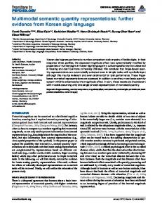
(a) Start from the expansion point P,jk of the triangle [Vi, Vj, Vk] and directional expansion J say z =::: ¢(x,y). Choose one point Q on the T-plane at Pijk within the convergence radius, such that Q is on the middle-perpendicular line of [T(Vi), T(Vj)] and as far as possible from T(Pijk). (b) Refine the point (Q, z(Q)) to a point on the surface, say Ql. The point Ql becomes a new expansion point. Compute directional expansion at Ql, say z =::: ¢iJ(x,y), and its circle ofconvcrgence. The triangulation around Ql is reconstructed as follows . • Let [ViJ lI/] and [Vj, Vm ] be the neighboring edges of [Vi, Vi]· Then on the T-plane at point QlI if the angle < T(Vi)T(Vi)T(lI/) 2: ~ and < T(Vi)T(Vi)T(Vm ) ~ I or the convergence circle has no intersection points with [T(Vi)J T(lI/)] and [T(Vj), T(Vm )], then choose the intersection point Q2 of the circle and the perpendicular line of[T(Vi), T(Vj)] passing through T(QI). If (T(QJ), Q2) intersects a previous edge or the bounding box, then Q2 is chosen to be this intersection point. Refine (Q2,¢iJ(Q2)) and obtain a new vertex VII and form the new triangle [Vi, Vj, VII]' Also see top part of Figure 5. • If the angle < T(Vi )T(Vi)T(V/) < t and (T(Vi), T(Vj)) intersect the circle (or, angle < T(Vi)T(Vj )T(Vm ) < ~ and (T(Vj),T(Vm )) intersects the circle), (see middle part of Figure 5, then take QJ as this i'i,tersection point. Otherwise take Q1 ::;: T(lI/). In the first case, we add a point on the edge [Vi, Vi] and divide it into two edges, [Vi, V] and [VS, Vot ]. The [V2, Vot ] is expansible and [V2, Vs] is not. A new expansible edge [Vb VsJ is produced. In the second case, edge [Vi, Vj] and [Vi, lI/] become non-expansible and a new expansible edge [Vi, Vi] is generated. A related case is shown in the bottom part of Figure 5 and is handled in much the same fashion.
3. Final Ste.p. We iterate the General Step, until every edge is non-expansible for that real component. Figure 6 shows the triangulation of implicitly defined polynomial surfaces. 3.0.2
Rational Parametric Surfaces
A well-known strength of the parametric representation (its mapping from m? to m.3 ) is the ease by which real points can be generated on the parametric curve or surface. However the problem of constructing triangulations with consistent topology is still highly non-trivial. Arbitrary rational parametric surfaces have real pole curves in their domain, where the denominators of the parameter functions vanish, domain real base points for which all four numerator and denominator polynomials vanish simultaneously, and other features that cause naiive
................. /...
/.....
:::.~ 0
.••
,
:.
.....
.
~~
••••••••••• /':••
.... O-------~"' .... ! V~'" .
V .' .. .:l
.
··
~::~
n
.'\.~.. :.:/~\ ........ \./ '
...
.
•
••• _. __ •••••
.
'••!O---':::':'-"::"'~' 0'..... -••••••
...
".•••••••••••••••••i(j.'j
••••••••••••••••"'ij j
.'.
.
....... .:.........
/ ··v .:.
,
.."
."
..
~
. '.••••
.
·
· ...
If.k'"
'.
'"
0' '.
•••••••••
"'.
Q
J
".
••••
v,
e
;
.:
:.!.' / 0'
••••••••••••••••>tf,J j
..:::-J:."
~.
:/ ;.
....
.. -.....: '"!' · .. •••":j
'0....."l,v h
k
..
"'. .~ "
".
;.......
••••
•••••
,
'",
..........:..//•............ ...
..." ...
................i(j j
•••• , V;
/"
1••::::.::•••
-_
0'-
•
..,/
.,:
.,/
:
••.. Vk""
0"
....... Q
..'
..
.....
V e
"
i
l .,
.
" .,'
"
:... . • •
.. '.
;.::.~
·····V·····:·r;::····
.~",
l'
.
..
"" '.
' " 0".
V':
e,.
........" \ ...... : V.!
:.....
.I
/.,. :~-
.. -_
V····... . ."j k ••••••••••••• 'V •.••
"~
Figure 5: Expansion Steps for the Surface 'Triangulation
......•
' :
f.....
.
.r
Figure 6: Surface Triangulations of an Implicitly Defined Sphere, Cubic Elbow and a Torus 'VI
I /ff-~!~-=
, I
I
~. \
\
II
I,
II
I,'I
I
Figure 7: A Quadratic Parametric Surface with Domain Poles polygonal approximation algorithms to fail. These are ubiquitous problems occurring even among the natural quadrics. See examples shown in Figures 7 and 8. In geometric design and graphics, where rational Bezier and B-spline surfaces have become popular, the above problems have so far been avoided by a restriction to smooth rational surface patches with denominator polynomials having all positive coefficients [32, 58] (i.e. no real poles or real base points). Sophisticated but unsuspecting triangulation techniques which accept arbitrary rational parametric input (e.g. those implemented in Maple V, Mathematica, Mac5yma) produce completely unintelligible results. Dur second algorithm provides a complete and general solution to this problem. We first illustrate the topological problems that arise if one naively mapped a triangulation from the (5, t) domain to the surface in (x, y, z) space, using the rational parametric equations. 1. [Finite Parameter Range] To fully cover the parametric curve or surface, one must allow the parameters to somehow range over the entire parametric domain, which is infinite. For example, the unit sphere f( x, y, z) = x 2 + y2 + z2 - 1 = 0 has the standard rational parametric representation (x = 1+J2;+I~' Y =
Figure 8: A Cubic Parametric Surface with Seam Curves Due to Base Points
l+.'2~I+t" values
8
Z = ~+;~+:~) In this parameterization the point (0,0, -1) can only be reached by the parameter = t = 00.
2. [Poles] Even when restricting the surface to a bounded real part of the parametric domain, the rational functions describing the surface may have poles over that domain. A hyperboloid of two sheets, with implicit equation z2 + yz + xz - y2 - xy - 2: 2 - 1 = 0, has the parametric representation (X(8, t) = " ( t) -- sr~+6.1+S.2 " ( t) -- St'+6.t-2r+s'~-2'+1) th en pro blems arise . because 0 £the 51"+6Jt+S.~ l'y S, l'Z s, St"+6.I+S." 1
pole curve described by 5t 2 + 6st + 5s 2
-
1 = 0 in the parameter domain. See Figure 7.
3. [Base Points] The rational parameter functions describing curves and surfaces are generally assumed to be reduced to lowest common denominators, i.e., the numerator and denominator of each rational function are relatively prime. Thus for a curve, there is no parameter value that can cause both numerator and denominator of a rational parameter function to vanish. For surfaces, the situation is different. For the general parametric representation stated earlier, even if !I,f2,h.f