Population Density and Spatial Distribution Pattern ... - Semantic Scholar
Recommend Documents
on these four bean species using variance to mean ratios, Taylor's power law coefficients and Iwao's ... 1999; Southwood and Henderson, 2000). Sampling ...
through index of dispersion, Lloyd's mean crowding, Morisita's index as well as through .... of dispersion and finally Lloyd's mean ..... and Hall, London, 524 PP.
of Taylor's power law on Zane, Sahar, Williams and Tellar varieties ... distribution of T. tabaci on Sari, Zane, Williams and Tellar varieties as well as on Ks3494.
Precaution in the harvest of Methuselah's clams; the difficulty of getting timely feedback from slow- paced dynamics. Canadian Journal of Fisheries and Aquatic.
Jun 23, 2013 - values were 0.345 and 0.212 (at landscape and sampling site). These suggest .... mation Authority (NAMRIA), Taguig City, Metro Manila. All.
ent on the population density of ragweed (Reznik,. 1985; Reznik et al., 1990). The present work was de- voted to the analysis of new data that had been col-.
Sep 1, 2017 - Ni Li1,2â¯, Qi Chen1,2â¯, Jie Zhu1,2, Xing Wang1,2, Jian-Bin Huang2, Guo-Hua ..... Investigation: Ni Li, Qi Chen, Jie Zhu, Jian-Bin Huang.
Bouboulis generously assisted in the field and nick ernst provided technical support. ... Hines, J. Fallon, K. l. pardieck,. D. J. Ziolkowski, Jr., & W. a. link. 2011. the.
Analysis System (SeaDAS version 5.1.6) software, following ... densidad. 3Golden Software, LLC. ..... logistical and diving team support for this project.
Feb 12, 2016 - 2National Center for Earth-surface Dynamics and St. Anthony Falls ...... uniformity of the concentration is not so well established transversely.
1874-1967/09. 2009 Bentham Open. Open Access. Density-Dependent Individual and Population-Level Metabolic Rates in a. Suite of Single-Celled Eukaryotes.
Mar 5, 2014 - 2840 people per sq km), Brzeg (2330), Kluczbork. Table 1. Spatial regression coefficients. Population/Parameter. Regression coeff. Stand. dev.
tion density (Gilbert 1992, 2002, 2003a; Schröder & ... stimulus is taxonomically specific (Gilbert 2003a). .... 1993; Folt & Burns 1999; Hembre & Megard 2003).
Mar 26, 2017 - commonLeopard,RhesusMacaque,AsfiaficJackal,Red ..... International Snow Leopard Trust, and Wildlife Conservation Society. (India Program) ...
Byrne, 1993; Preston, 1993; Powell and. Gibbs, 1995). .... thuria mexicana were collected in Pondsack. (09°1719N ..... Powell, J.R., and J.P. Gibbs. 1995.
Dec 20, 2012 - FZT infection of fish should include not only intra-pond snail control, but also include water sources of allochthonous cercariae ..... Report of a Joint FAO/NACA/WHO Study Group. ... Parasitology Research 101: 1277â1284. 11.
engineering community [1]. EEG captures the electric field generated by the central ... H. Lu, H.-L. Eng, and C. Guan are with Institute for Infocomm Research,. Singapore. ...... Engineering from Florida Institute of Technology in. 1992 and 1994 ...
Mar 28, 2017 - Dopamine signaling tunes spatial pattern selectivity in C. elegans. Bicheng Hanâ , Yongming Dong, Lin Zhang, Yan Liu, Ithai Rabinowitch, ...
mutant strains of yeast [9] and coral reef invertebrates [10]. ... Each node can either host one individual of a given s
Jun 27, 2014 - Kumari S, Mg S, Mayor S (2010) Endocytosis unplugged: multiple ways .... Zerial M (2005) Kinase-regulated quantal assemblies and kiss-and-.
During 2013 we conducted 600 transects in Eastern Romania for European ... information will contribute to Natura 2000 sites management and development, but also for .... The transects were randomly chosen using Quantum GIS software,.
SciRP.org/journal/jgis). Heavy Metals' Spatial Distribution Characteristics in a. Copper Mining Area of Zhejiang Province. *. Hua Sun1, Juan Li1, Xiaojun Mao2.
Mar 4, 2014 - processing, and marketing activities, while 3.5 million people benefit .... The measurement tool was calibrated before area calculation ... It is an important parameter considered in installation of drip irrigation systems in.
Population Density and Spatial Distribution Pattern ... - Semantic Scholar
the spatial distribution pattern of this pest, data were analyzed through index of dispersion, Lloyd's mean ... Sampling programs can be used in assessing crop ... method (Kuhar et al., 2003), sweep-net sampling (South- ..... Wiley, New York.
Available online at www.notulaebotanicae.ro Print ISSN 0255-965X; Electronic 1842-4309 Not Bot Horti Agrobo, 2011, 39(2):42-48
Notulae Botanicae Horti Agrobotanici Cluj-Napoca
Population Density and Spatial Distribution Pattern of Hypera postica (Coleoptera: Curculionidae) in Ardabil, Iran Mona MORADI-VAJARGAH1 , Ali GOLIZADEH1* , Hooshang RAFIEEDASTJERDI1 Myron P. ZALUCKI2 , Mehdi HASSANPOUR 1 , Bahram NASERI1 1
University of Mohaghegh Ardabili, Faculty of Agriculture, Department of Plant Protection, Daneshgah Street, P.O.Box 179, Ardabil, Iran; [email protected] (*corresponding author) 2
The University of Queensland, School of Biological Sciences, St. Lucia, Queensland 4072, Australia
Abstract The alfalfa weevil, Hypera postica (Gyllenhal), feeds almost exclusively on alfalfa, Medicago sativa L. in most region of the world where forage crop is grown. It has been investigated the population density and spatial distribution of alfalfa weevil on alfalfa in Ardabil during 2010. Using a 0.25 m2 quadrate sample unit a reliable sample size was 65, with maximum relative variation of 15%. The relative variation (RV) of the primary sampling data was 13.6. The highest population density of the alfalfa weevil was recorded on 17th April. To estimate the spatial distribution pattern of this pest, data were analyzed through index of dispersion, Lloyd’s mean crowding, Morisita’s index and two regression models (Taylor’s Power Law and Iwao’s Patchiness Regression). Taylor’s model showed an aggregated distribution pattern for all life stages. Iwao’s patchiness regression indicated that larvae, adult and total life cycle had aggregated spatial distribution (tc < tt), while pupae of alfalfa weevil exhibited a random pattern. The index of dispersion and Lloyd’s mean crowding methods indicated an aggregated distribution for this insect. Spatial distribution parameters of this species are used to outline a sampling program as well as to estimate population density of H. postica development stages. Optimum sample sizes for estimates of larval density, at three levels of precision, are presented. Keywords: alfalfa weevil, distribution pattern, Iwao’s patchiness regression, population fluctuation, sampling program, Taylor’s power law Introduction
Alfalfa or lucerne, Medicago sativa L., is one of the important forage crops cultivated in most regions of the world. It is an extremely adaptable plant and can be grown under a broad range of environmental conditions. The crop is attacked by a diversity of insect pests with the alfalfa weevil, Hypera postica (Gyllenhal), the most destructive pest of alfalfa in the world (Metcalf and Luckman, 1994). Hypera postica is a typical oligophagous insect that feeds almost exclusively on leguminous plants of the genus Medicago, although it occasionally may feed on a few species of related genera including: Melilotus, Trifolium, and Trigonella in most region of the world where alfalfa is grown. Both larvae and adults of alfalfa weevil are voracious feeders damaging terminals, foliage and new crown shoots. Fields heavily infested may appear silver or white, as most leaves are skeletonized or consumed entirely. Severe weevil pressure can totally destroy plants (Fick, 1976). In Iran, Afshar (1937) reported alfalfa weevil, known as Phytonomus variabilis (Herbest), for the first time. In addition he described its morphological characteristics, distribution and agricultural importance (Karimpour, 1994). Injury levels caused by H. postica are not exactly clear in Iran but there is a re-
port that 60% of alfalfa damage belongs to alfalfa weevil (Khanjani and Pourmirza, 2004). According to studies in Iran, among alfalfa pests, H. postica is the most important, as all its life stages feed on alfalfa leaves and stems, but the main damage is caused by 3rd and 4th instars. If there are more than 50 larvae of different instars/m2 in a field, all leaves of alfalfa will be destroyed and the whole of field will have a white appearance. Sometimes feeding activity of alfalfa weevil leads to total destruction of alfalfa crop especially in its first harvest (Karimpour, 1994). Estimating population densities of pest arthropods is the most important part of basic research in agricultural ecosystems and one of the main components in pest management programs (Kogan and Herzog, 1980); many other properties are derived from the density measure (Pedigo and Buntin, 1994). A reliable sampling program to estimate density should include a proper sampling time, sampling unit and sampling size in which the determination of spatial distribution is crucial (Boeve and Weiss, 1998; Pedigo and Buntin, 1994; Southwood and Henderson, 2000). Sampling programs can be used in assessing crop loss (Hughes, 1996), studying the population dynamics of pests ( Jarosik et al., 2003; Wilson, 1994) and determination of levels of pest infestation in order to apply control
Moradi-Vajargah M. et al. / Not Bot Horti Agrobo, 2011, 39(2):42-48
43
measures (Arnaldo and Torres, 2005). Although the objectives of population sampling could differ, the development of a sampling procedure requires knowledge of the spatial distribution of the populations (Binns et al., 2000; Liu et al., 2002; Southwood, 1978). Knowledge of the spatial distribution of insects is important in understanding the biology and ecology of a species and the basis for the development of sampling protocols (Bins and Nyrop, 2000). Several methods are employed in the sampling of alfalfa weevil species in crops, some of them being the washing method (Kuhar et al., 2003), sweep-net sampling (Southwood, 1978), and the plastic-bag shake method (Higgins et al., 1991). The latter is the most commonly recommended (Kuhar et al., 2003). Methods that are commonly used to describe dispersion of arthropods populations have been summarized by Southwood (1978). Several estimates based on the dispersion parameter k of the negative binomial distribution and on the relationship between variance and mean are used as indices of aggregation (Davis, 1994; Krebs, 1999; Ludwig and Reynolds, 1988; Southwood, 1978). Sampling plans based on these indicators can minimize variation of sampling precision (Kuno, 1991). Having information about density and changes in population of H. postica during the season, identification of factors affecting population fluctuations and determination of their effects will help alfalfa producers in management of this pest. Knowing the spatial distribution of an insect pest is central to design of a management program (Cho et al., 2001; Wearing, 1988). Many of these aspects of pests ecology may be region specific, so it is necessary to do this study in Ardabil region where there is no reported similar research. Hence, population changes of alfalfa weevil and its distribution pattern were determined in the current study. Materials and methods
The present study was conducted in an experimental field of Mohaghegh Ardabili University in the suburb of Ardabil, Iran from April to August 2010. A field of 5000 m2 was selected for sampling. Irrigation was performed on a weekly basis. Plants were grown using standard agronomic practices recommended for Ardabil region. No insecticides were applied to the field for alfalfa weevil control in the spring of 2010. Development of sampling plans A sampling quadrate was selected as a sample unit as developed by Hilburn (1985). The density of different biological stages of alfalfa weevil was estimated by sampling twice a week from March to August until first alfalfa harvest. On average 65 samples of plant matter were collected from the field using a 0.25 m2 sampling quadrate and were shaken into a bag to expose alfalfa weevil larvae, pupae and adults for counting (Kuhar et al., 2003), so the number of
alfalfa weevils life stages were recorded. A sub-sample of 20 shaken stems was placed in a modified Berlese funnel to estimate the proportion of larvae remaining on stems after the plastic bag shake method for each sample (Higgins et al., 1991). This proportion was added to the total larval density of each sample. The fundamental principle of random sampling was observed so that all locations could have an equal chance of being sampled. This was achieved by moving in field diameters. Relative variation (RV) was employed to assess the effectiveness of the sampling method. RV for the sampling data was calculated as follows: RV=(SE/m)100 , where SE is standard error of mean and m is the mean of primary sampling data. The reliable sample size was determined using the following equation: N=(ts/dm)2, where, N = sample size, t = t-student, s = standard deviation, d = desired fixed proportion of the mean and m = the mean of primary data (Pedigo and Buntin, 1994). Spatial distribution pattern The spatial distribution of H. postica among the 65 sample units was determined by five commonly used methods: index of dispersion, Taylor’s power law, Iwao’s patchiness regression, Morisita’s coefficient of dispersion and finally Lloyd’s mean crowding. Index of dispersion Dispersion of a population can be classified through a calculation of the variance to mean ratio; namely: s2/m=1 random, < 1 regular and > 1 aggregated. Departure from a random distribution can be tested by calculating the index of dispersion (ID), where n denotes the number of samples: ID = (n-1)s2/m ID is approximately distributed as x2 with n-1 degrees of freedom. Values of ID which fall outside a confidence interval bounded with n-1 degrees of freedom and selected probability levels of 0.95 and 0.05, for instance, would indicate a significant departure from a random distribution. This index can be tested by Z value as follows: Z = 2I D - (2ν - 1) , ν = n - 1
If 1.96 ≥ Z ≥ -1.96, the spatial distribution would be random but if Z < - 1.96 or Z > 1.96, it would be uniform and aggregated, respectively (Patil and Stiteler, 1974). Lloyd’s mean crowding (x*) Mean crowding (x*) was proposed by Lloyd to indicate the possible effect of mutual interference or competition among individuals. Theoretically mean crowding is the mean number of other individuals per individual in the same quadrate: x*=m+s2/m-1 As an index, mean crowding is highly dependent upon both the degree of clumping and population density. To remove the effect of changes in density, Lloyd introduced the index of patchiness, expressed as the ratio of mean
Moradi-Vajargah M. et al. / Not Bot Horti Agrobo, 2011, 39(2):42-48
44
crowding to the mean. As with the variance-to-mean ratio, the index of patchiness is dependent upon quadrate size x*/m=1 random, 1 aggregated (Lloyd, 1967). Morisita’s coefficient of dispersion (Iδ) Reasoning that the diversity of numbers of individuals per quadrate could be used as a measure of spatial pattern, Morisita (1962) developed the index Iδ. Suppose n quadrates are sampled and xi represents the number of individuals in the ith quadrate. Define δ as the probability that individuals of a randomly drawn pair will come from the same quadrate. If the xi came from a random or poisson distribution, the expected value of δ is 1/n. Then the index Iδ can be defined as the ratio of δ to its expected value assuming a random distribution. Values for Iδ may range from 0 to n and N is the total number of individuals sampled in n quadrate. Iδ is calculated as follows and used to classify population: Σx (x - 1) I =n i i δ N(N - 1)
To determine if the sampled population significantly differs from random, the following large sample test of significance can be used: Z=(Iδ-1)/(2/nm2)(1/2), where m = mean population density per leaf in each sampling date and n = the number of sample units. By comparing the value of Z with tabulated values for a random distribution and reject the hypothesis that the sampled population is dispersed |Z|>z(α/2)randomly if (Pedigo and Buntin, 1994). Regression methods For many insect and animal species, Taylor (1961) found that a power law function could be used to model the relationship between mean and variance as: s2=amb , where s2 is the variance; m the sample mean; a is a scaling factor related to sample size and b measuring the species aggregation. When b = 1, < 1 and > 1, the distribution is random, regular and aggregated, respectively. Through use of a log transformation, one can estimate the coefficients with linear regression as: log(s2)=log(a)+blog(m) , where a and b are the parameters of the model, estimated by linearizing the equation after a log-log transformation (Taylor, 1961). Iwao’s patchiness regression method was used to quantify the relationship between mean crowding index (m*) and mean density (m) using the following equation: m*=α+βm , where α indicates the tendency to crowding (positive) or repulsion (negative) and β reflects the distribution of population in space and is interpreted in the same manner as b of Taylor’s power law (Iwao and Kuno, 1968). Student t-test can be used to determine whether the colony is composed of single individuals and if colonies are dispersed randomly.
Test b = 1: t=(b-1)/SEb and Test β = 1: t=(β-1)/SEβ, where SEb and SEβ are the standard errors of the slope for the mean crowding regression. Calculated values are compared with tabulated t-values with n-2 degrees of freedom. If the calculated t (tc) < t-table (tt), the null hypothesis (b = 1) would be accepted and spatial distribution would be random. If tc> tt, the null hypothesis would be rejected and if b > 1 and b < 1, the spatial distribution would be aggregated and uniform, respectively. Optimum number of sample units (sample size) The optimum sample size is the smallest number of sample units that would satisfy the objectives of the sampling program and achieve the desired precision of estimates. Finding out the Taylor power law and Iwao’s regression coefficients eliminates experimental needs for large sample size (Ifoulis and Savopoulou-Soultani, 2006). The optimum number of sample units was derived from formula 2
using Iwao’s regression method coefficients (Buntin, 1994; Young and Young, 1998), where D represents the range of accuracy, a and b is Taylor regression coefficients, α and β is Iwao’s equation coefficients and m is mean density of populations and t α/2 is t-student. It has been calculated the optimum number of sample units with 15, 20, and 30% confidence interval levels and plotted them using excel program. Results and discussion
Sampling and population fluctuation The results from primary sampling showed that the reliable sample size with maximum variation of 15% was 20 samples during the early season and an average of 65 samples during growing season. The relative variation (RV) of the primary sampling data was 13.6, which is suitable for a sampling plan. Rainfall and climatic conditions in the early growing season caused the first sampling date to be 12 April. The population increased from the beginning date and after a week reached a peak by 17 April at 619 larvae per quadrate (Fig. 1). Then the population decreased sharply in the following week. Thereafter, the population continued to decrease until the end of the growing season. No H. postica were observed after 20 July (Fig. 1). In developing a sampling program for research or management purposes, it is necessary to determine two characteristic features of any population, its density as well as its dispersion (Pedigo and Buntin, 1994). Alfalfa weevil
Moradi-Vajargah M. et al. / Not Bot Horti Agrobo, 2011, 39(2):42-48
45
population density showed a rising trend during the early growing season with small larva, first and second instars, constituting the bulk of the population. The highest population density during the April could be attributed to unfavorable climatic conditions for natural enemies and high quality of host plant. As the season progressed the reduction in host plant quality and higher activities of alfalfa weevil biocontrol agents could have led to a decreasing population. Moreover, the early high density of larvae caused a significant reduction of leaf and young stems in the alfalfa field and this could be another reason for the following reduction in population density. Along with warming weather and reducing humidity, population density decreased reaching near to zero per sampling unit. The last observation of beetle was made by last week of July. Considering the changes in H. postica density, it is possible that timing the first cutting of alfalfa to coincide with peak alfalfa weevil populations may be a suitable means of control. Thus, in order to reduce population density, any effective pest management strategies should be applied during the early growing season against H. postica.
Fig. 1. Population fluctuation of Hypera postica in alfalfa (mean ± SE) during the growing season in 2010 in Arabil, Iran. Each estimate is based on 65 random 0.25 m2 quadrates
Spatial distribution pattern “The variance to mean ratio” were greater than unity indicating that the spatial distribution of alfalfa weevil stages in alfalfa field is aggregated (Tab. 1); the calculated Z-values of each stage was significantly greater than 1.96. The aggregated distribution suggests that the presence of an individual at one point leads to an increased probability of another individual being close. The Lloyd’s mean crowding were calculated for H. postica life stages and x*/m ratio ranged from 1.08 to 2.66 (Tab. 1). Similar conclusions can be made from the results of Lloyd’s mean crowding for alfalfa weevil life stages distribution which indicated that H. postica had an aggregated distribution on alfalfa. The use of dispersion indices seem to be convenient decision making methods for management programs because of their easy calculation procedure and simple results (Darbemamieh et al., 2011).
Tab. 1. Estimated parameters by variance to mean ratios and Lloyd’s mean crowding methods for life stages of Hypera postica in 2010 Larvae Pupae Adult Variance to mean ratio S2/m ID Z
64.530 1290.611 44.560
x* x*/m
88.52 1.76
3.303 69.374 5.376
4.286 42.865 4.900
Total 63.440 1712.902 51.25
Lloyd’s mean crowding 1.74 2.66
1.21 1.08
103.96 1.71
The Morisita’s index (Iδ) values for all sampling dates and for three life stages and total life span of H. postica is significantly greater than 1 (Tab. 2), indicating the spatial distribution of this pest was aggregated at most sampling dates. As Morisita’s coefficient estimates spatial distribution pattern using the mean and variance of each sampling date separately, so this index is more perfect than dispersion index. The detailed knowledge of dispersion in different time intervals during growing season would be useful for research strategies more than management programs (Darbemamieh et al., 2011). Although, the spatial pattern of alfalfa weevil in all sampling date was aggregated pattern, changes in distribution pattern during season could be casued by changes in population density or movement of larva from the clumped egg locations (Pedigo and Buntin, 1994). According to Taylor’s model (Tab. 3), the calculated intercepts (a) for larvae, pupae, adult and total stages of H. postica were greater than zero (a = 3.27, 2.58, 3.10 and 3.14 respectively) and all b values from Taylor’s power law were significantly >1, indicating an aggregated dispersion pattern of H. postica stages (Tab. 3). There were significant relationship between log S2 and log m for all life stages of H. postica. Moreover, the coefficients of determination for the Taylor’s power law ranged from 0.867 to 0.977 (Tab. 4). Similar to Taylor’s power law, Iwao’s patchiness regression produced comparable results for the distribution of alfalfa weevil. Iwao’s patchiness regression adequately described the relationship between mean crowding (x*) and mean density (m) for life stages of H. postica (P1 for larvae, adult and as well as for total life span, indicating that larvae and adult weevils tend to be aggregated. Although the slope of Iwao model (b) was greater than unity for pupae stage, it is not significantly different from 1 (tc < tt), indicating that pupae of H. postica are randomly distributed in the sampling area. This differs from other analysis methods used in this study.
Moradi-Vajargah M. et al. / Not Bot Horti Agrobo, 2011, 39(2):42-48
46
Tab. 2. Parameters of Morisita’s index and Z calculated for Hypera postica on Alfalfa in 2010 for each sampling date Larvae
Since in regression methods the mean and variance of each sampling time was used separately, therefore the Taylor’s power law and Iwao’s patchiness were more accurate than the variance to mean ratio method. The two regression techniques (Taylor’s Power Law and Iwao’s patchiness regression) have been widely used to evaluating dispersal, data normalizing for statistical analysis, and developing sampling protocols for many insects (Davis, 1994; Deligeorgidis et al., 2002). The varied conclusions for dispersion of a life stage pattern from two regression methods suggest that different statistical methods accuracy in calcu-
lating the spatial distribution could be different. Based on Southwood (1978), when a population in an area becomes sparse, the chance of an individual occurring in any sample unit is so low that the distribution is in effect random. Spatial distribution of the alfalfa life stages using different analytical methods all indicated an aggregated pattern. This behavior has been mentioned for many other insects and mites (Darbemamieh et al., 2011; Geiger and Daane, 2001; Hamilton and Hepworth, 2004; Sedaratian et al., 2010). Zahiri et al. (2006) analyzed the spatial distribution of alfalfa weevil and some of its’ natural enemies by Taylo’s
Tab. 3. Spatial Distribution of Hypera postica on alfalfa during 2010 using Taylor’s power law analysis
Tab. 4. Spatial Distribution of Hypera postica on alfalfa during 2010 using Iwao’s patchiness regression analysis
Life stages Larvae Pupae Adult Total
a
3.273 2.582 3.097 3.140
b
1.355 1.300 1.416 1.288
SE b
0.089 0.090 0.068 0.096
r2adj
0.920 0.908 0.977 0.867
P reg 0.00 0.00 0.00 0.00
tc
3.988 3.333 6.117 3.00
tt
2.093 2.086 2.262 2.056
Life stages Larvae Pupae Adult Total
α
4.276 1.023 0.151 5.754
β
1.148 1.467 2.370 1.116
SE β
0.035 0.252 0.105 0.036
r2adj
0.974 0.609 0.946 0.972
P reg
tc
0.00 4.228 0.00 1.853 0.00 13.047 0.00 3.222
tt
2.093 2.086 2.262 2.056
Moradi-Vajargah M. et al. / Not Bot Horti Agrobo, 2011, 39(2):42-48
47
power law in Hamedan, west Iran and reported clumped dispersion patterns for life stage of H. postica and random dispersion for its natural enemies. Muker and Guppy (1972) considered H. postica to be aggregated on alfalfa which is the same as the present result. Despite parameters such as rate of population growth and reproduction that vary from one generation to another, spatial distribution is partially constant and is a characteristic of the species (Taylor, 1984). The behavioral patterns and environment could be determinant the spatial distribution of population individuals in an ecosystem. Different plant varieties can affect the spatial distribution of an insect (Sedaratian et al., 2010), therefore, further work is needed to verify the spatial distribution of this pest in commercial alfalfa fields and on different varieties of alfalfa. The dispersion pattern of alfalfa weevil identified in this study can be used in sampling program as well as in proper estimation of their population densities in protection management of alfalfa.
Optimal sample size
Optimum number of sample units The optimal sample size was calculated using Taylor’s and Iwao’s coefficient, and the relationship between optimum number of sample unit and mean number of H.
Mean larvae per sample unit Fig. 2. Relationship between optimal sample size (0.25 m2 quadrates) and mean number of Hypera postica larvae, for three levels of precision, based on Taylor’s power law (A) and Iwao’s regression method (B) coefficient
postica larvae, for 15, 20 and 30% level of precision was calculated (Fig. 2). Comparison of the two different formulae used for calculating the optimal sample unit size showed a similarity between the lines calculated using the both regression methods (Fig. 2). The optimal sample size suggested by each model is typically higher at low population levels. The lower estimate of the sample size was calculated by using Taylor’s equation, for larval stages. Principally, Taylor’s method reduces the necessary sample size when compared with Iwao’s method (Darbemamieh et al., 2011; Ifoulis and Savopoulou-Soultani, 2006). Taylor’s power law model usually better fits the spatial dispersion than Iwao’s model to accomplish a desired precision of estimates (Afshari et al., 2009). These different precision levels (three lines) adopted in this study, could be chosen for ecological or insect behavioral studies. In order to acquire a higher level of precision the 15% level could be adopted, whereas in IPM programs 20% or 30% level would be acceptable. References Afshari A, Soleyman-Negadian E, Shishebor P (2009). Population density and spatial distribution of Aphis gossypii Glover (Homoptera: Aphididae) on cotton in Gorgan, Iran. J Agr Sci Tech 11:27-38. Arnaldo PS, Torres LM (2005). Spatial distibution and sampling of Thaumetopoea pityocampa (Lep: Thaumetopoeidae) populations of Pinus pinaster Ait. in Montesinho, N. Portugal. Forest Ecol Manage 210:1-7. Binns MR, Nyrop JP, Werf W (2000). Sampling and monitoring in crop protection: The theoretical basis for developing practical decision guides. CABI Publishing, UK. Boeve PJ, Weiss M (1988). Spatial distribution and sampling plans with fixed levels of precision for cereal aphids (Homoptera: Aphididae) infesting spring wheat. Can Entomol 130:67-77. Buntin GD (1994). Developing a primary sampling program, 99-11 p. In: Pedigo LP, Buntin GD (Eds.). Handbook of sampling methods for arthropods in agriculture. CRC, Boca Raton, FL. Cho K, Lee JH, Park JJ, Kim JK, Uhm KB (2001). Analysis of spatial pattern of greenhouse cucumbers using dispersion index and spatial autocorrelation. Appl Entomol Zool 36(1):25-32. Darbemamieh M, Fathipour Y, Kamali K (2011). Population abundance and seasonal activity of Zetzellia pourmirzai (Acari: Stigmaeidae) and its preys Cenopalpus irani and Bryobia rubrioculus (Acari: Tetranychidae) in sprayed apple orchards of Kermanshah, Iran. J Agr Sci Tech 13:143-154. Davis PM (1994). Statistics for describing populations, 33-54 p. In: Pedigo LP, Buntin GD (Eds.). Handbook of sampling methods for arthropods in agriculture. CRC Press, Boca Raton, Florida.
Moradi-Vajargah M. et al. / Not Bot Horti Agrobo, 2011, 39(2):42-48
48
Deligeorgidis PN, Athanassiou CG, Kavallieratos NG (2002). Seasonal abundance, spatial distribution and sampling indices for thrips populations on cotton; a four year survey from Central Greece. J Appl Entomol 126:343-348. Fick GW (1976). Alfalfa weevil effects on regrowth of alfalfa. Agron J 68:809-812. Geiger CA, Daane KM (2001). Seasonal movement and distribution of the grape mealybug (Homoptera: Pseudococcidae): developing a sampling program for San Joaquin valley vineyards. J Econ Entomol 94:991-301. Hamilton AJ, Hepworth G (2004). Accounting for cluster sampling in constructing enumerative sequential sampling plans. J Econ Entomol 97:1132-1136. Higgins RA, Rice ME, Blodgett SL, Gibb TJ (1991). Alfalfa stem-removal methods and their efficiency in predicting actual numbers of alfalfa weevil larvae (Coleoptera: Curculionidae). J Econ Entomol 84:650-655. Hilburn DJ (1985). Population dynamics of overwintering life stages of the alfalfa weevil, Hypera postica (Gyllenhal). Virginia Polytechnic Institute and State University, PhD Diss. Blacksburg. Hughes GM (1996). Incorporating spatial pattern of harmful organsim into crop loss models. Crop Prot 15:407-421. Ifoulis AA, Savopulou-Soultani M (2006). Developing optimum sample size and multistage sampling plans for Lobesia botrana (Lepidoptera: Tortricidae) larval infestation and injury in Northern Greece. J Econ Entomol 99:18901898. Iwao S, Kuno E (1968). Use of the regression of mean crowding on mean density for estimating sample size and the transformation of data for the analysis of variance. Res Popul Ecol 10:210-214. Jarosik V, Honek A, Dixon AFG (2003). Natural enemy ravine revisited importance of sample size for determining population growth. Ecol Entomol 28:85-91. Karimpour Y (1994). Studies on the effect of different insecticides on alfalfa weevil (Hypera postica) and etrimfos residues in green alfalfa. Tarbiat Moddares University, MSc Thesis, Tehran. Khanjani M, Pourmirza AA (2004). A comparison of various control methods of alfalfa weevil, Hypera postica (Col: Curculionidae) in Hamadan. J Entomol Soc Iran 1:67-81. Kogan M, Herzog DC (1980). Sampling methods in soybean entomology. Springer Verlag, New York. Krebs CJ (1999). Ecological methodology. 2nd ed. Addison Wesley Longman Inc, New York. Kuhar TP, Youngman RR, Laub CA (2003). Alfalfa weevil (Coleoptera: Curculionidae) population dynamics and mortality factors in Virginia. Environ Entomol 29(6):12951304.
Kuno E (1991). Sampling and analysis of insect population. Ann Rev Entomol 36:357-1971. Liu C, Wang G, Wang W, Zhou S (2002). Spatial pattern of Tetranychus urticae population in apple tree garden. J Appl Ecol 13:993-996. Lloyd M (1967). Mean crowding. J Anim Ecol 36:1-30. Ludwig JA, Reynolds JF (1988). Statistical ecology-a primer on methods and computing. John Wiley and Sons Inc, New York. Metcalf RL, Luckman WH (1994). Introduction to insect pest management. 3rd ed. Wiley, New York. Morisita M (1962). Iδ-index a measure of dispersion of individuals. Res Popul Ecol 4:1-7. Muker MK, Guppy JC (1972). Notes on the spatial pattern of Hypera postica (Coleoptera: Curculionidae) on alfalfa. Can Entomol 104:1995-1999. Patil GP, Stiteler WM (1974). Concepts of aggregation and their quantification: a critical review with some new results and applications. Res Popul Ecol 15:238-254. Pedigo LP, Buntin GD (1994). Handbook of sampling methods for arthropods in agriculture. CRC Press, Florida. Sedaratian A, Fathipour Y, Talebi AA, Farahani S (2010). Population density and spatial distribution pattern of Thrips tabaci (Thysanoptera: Thripidae) on different soybean varieties. J Agr Sci Tech 12:275-288. Southwood TRE (1978). Ecological methods with particular reference to the study of insect populations. 2nd ed. Chapman and Hall, London. Southwood TRE, Henderson PA (2000). Ecological methods. 3rd ed. Blackwell Sciences, Oxford. Taylor LR (1961). Aggregation, variance to the mean. Nature 189: 732-735. Taylor LR (1984). Assessing and interpreting the spatial distribution of insect populations. Ann Rev Entomol 29:321-357. Wearing CH (1988). Evaluating the IPM implementation process. Ann Rev Entomol 33:17-38. Wilson LT (1994). Estimating abundance, impact, and interactions among arthropods in cotton agroecosystems, 475-514 p. In: Pedigo LP, Buntin GD (Eds.). Handbook of sampling methods for arthropods in agriculture. CRC Press, Boca Raton. Young LJ, Young JH (1998). Statistical ecology: a population perspective. Kluwer Academic Publishers, Norwell, MA. Zahiri B, Fathipour Y, Khanjani M, Moharramipour S (2006). Spatial distribution of alfalfa weevil and its natural enemies in Hamedan. Proceeding of 17th Iranian Plant Protection. Karaj, Iran, 52 p.