Portfolio Selection Based on Distance between Fuzzy Variables

Hindawi Publishing Corporation Mathematical Problems in Engineering Volume 2014, Article ID 403208, 12 pages http://dx.doi.org/10.1155/2014/403208

Research Article Portfolio Selection Based on Distance between Fuzzy Variables Weiyi Qian and Mingqiang Yin College of Mathematics and Physics, Bohai University, Jinzhou 121000, China Correspondence should be addressed to Weiyi Qian; [email protected] Received 18 January 2014; Revised 8 April 2014; Accepted 24 April 2014; Published 19 May 2014 Academic Editor: Davide Spinello Copyright © 2014 W. Qian and M. Yin. This is an open access article distributed under the Creative Commons Attribution License, which permits unrestricted use, distribution, and reproduction in any medium, provided the original work is properly cited. This paper researches portfolio selection problem in fuzzy environment. We introduce a new simple method in which the distance between fuzzy variables is used to measure the divergence of fuzzy investment return from a prior one. Firstly, two new mathematical models are proposed by expressing divergence as distance, investment return as expected value, and risk as variance and semivariance, respectively. Secondly, the crisp forms of the new models are also provided for different types of fuzzy variables. Finally, several numerical examples are given to illustrate the effectiveness of the proposed approach.

1. Introduction Portfolio selection is to select a combination of securities among a large number of candidate securities which is the best to meet the investors’ goal. Markowitz [1] applied probability theory to portfolio selection problem and proposed the famous mean-variance model, in which expected return and variance were used to describe investment return and risk, respectively. Since then, variance has been widely accepted as a risk measure, and a great number of extensions have been proposed [2–5]. However, the mean-variance model has limited generality since variance considers high returns as equally undesirable as low returns. Variance becomes a deficient measure of risk when security returns are asymmetrical. Thus, Markowitz proposed semivariance as an improvement measure of risk, and numerous models have been developed based on semivariance such as models proposed in [6–10]. Generally speaking, the extension of Markowitz model is defined by minimizing the risk and maximizing the investment return. However, Kapur and Kesavan [11] introduced an entropy maximization model and a cross entropy minimization model. The objective of the entropy model is to maximize the uncertainty of random return and that of the cross entropy model is to minimize the divergence of the random return from a prior one. After that, many scholars accepted and explored these new models [12–15]. In the above literatures, security returns are considered as random variables. Since the security market is complex,

in many cases, security returns are hard to be well reflected by historical data. Therefore, many researches argued that we should find another theory to solve the portfolio selection problem in this situation. With the introduction of fuzzy set theory and credibility theory, many scholars began to employ them to describe and study fuzzy portfolio selection problems. Numerous models containing fuzzy variables are proposed. For example, Bilbao-Terol et al. [16], Gupta et al. [17], and Zhang et al. [18] extended the mean-variance model from different angles. Huang [19] developed fuzzy mean-variance models and further proposed fuzzy meansemivariance portfolio selection models [20]. Li et al. [21] employed skewness to describe asymmetry of fuzzy returns and further established fuzzy mean-variance-skewness models. Bhattacharyya et al. [22] proposed fuzzy mean-varianceskewness portfolio selection models by interval analysis. Huang [23] has used the entropy method to fuzzy environment to provide the fuzzy diversification models. In 2008, Li and Liu [24] proposed a concept of fuzzy entropy for measuring the uncertainty of fuzzy variables. Based on this concept, Huang [25] researched Kapur entropy maximization model in fuzzy environment. Moreover, the fuzzy cross entropy was given in [26] for measuring the divergence of fuzzy variables from a prior one. According to [26], Qin et al. [27] extended the Kapur cross entropy minimization model to fuzzy environment. These models in [27] were solved by using a hybrid intelligent algorithm which is designed

2

Mathematical Problems in Engineering

by integrating numerical integration, fuzzy simulation, and genetic algorithm. Distance between fuzzy variables is an important concept in fuzzy theory. Many scholars gave different definitions of distance between fuzzy variables, such as Hamming distance, Euclidean distance, and Minkowski distance. Recently, Tang et al. [28] gave a kind of definition of distance based on expected value operator of fuzzy variable. We define a new distance between fuzzy variables based on distance measure for interval numbers in this paper. Comparing to the distance measure of [28], the proposed distance measure can be calculated more easily. In this paper, our motivation is that the divergence of fuzzy investment return from a prior one is measured by using the proposed distance between fuzzy variables. Based on this idea, we establish two distance minimization models by defining investment return as expected value and risk as variance and semivariance, respectively. In addition, several crisp and simple equivalents of the optimization models are also proposed for different types of fuzzy variables. Finally, we compare our method with the methods presented by Chen et al. [29] and Wu and Liu [30] to demonstrate the effectiveness of the proposed approach. The remainder of the paper is organized as follows. Some preliminary concepts of credibility theory are briefly recalled in Section 2. The concept of distance between fuzzy variables is introduced in Section 3. In Section 4, we will propose two new models by minimizing distance between fuzzy variables. In Section 5, the crisp forms of the new models will be presented. Section 6 gives several numerical examples to illustrate availability of the proposed approach. Finally, a brief summary is given in Section 7.

2. Necessary Knowledge about Credibility Theory After Zadeh [31] initiated the concept of fuzzy set by membership function in 1965, he further indicated possibility theory [32]. Many research scholars, such as Dubois and Prade [33, 34], made their great contribution to its development. In 2002, B. Liu and Y.-K. Liu [35] defined a credibility measure to describe a fuzzy event. In order to develop an axiom system similar to the theory of probability, Liu founded the credibility theory in [36], which is a branch of mathematics for studying fuzzy phenomena. Further developments can be found in [37, 38]. Let 𝜉 be a fuzzy variable with membership function 𝜇. The credibility measure is defined as [35]

Cr {𝜉 ∈ 𝐵} =

1 (sub 𝜇 (𝑥) + 1 − sup 𝜇 (𝑥)) 2 𝑥∈𝐵 𝑥∈𝐵𝐶

(1)

for any set 𝐵 of real numbers. It is easy to see that credibility is self-dual.

In order to make a more general definition of expected value of a fuzzy variable, according to the credibility measure, B. Liu and Y.-K. Liu [35] defined the expected value of 𝜉 as 𝐸 [𝜉] = ∫

+∞

0

Cr {𝜉 ≥ 𝑟} 𝑑𝑟 − ∫

0

−∞

Cr {𝜉 ≤ 𝑟} 𝑑𝑟

(2)

provided that at least one of the two integrals is finite. If the fuzzy variable 𝜉 has a finite expected value, then its variance is defined as [35] 2

𝑉 [𝜉] = 𝐸 [(𝜉 − 𝐸 [𝜉]) ] .

(3)

Let 𝜉 be a fuzzy variable with finite expected value. Then the semivariance of 𝜉 is defined as [20] − 2

SV [𝜉] = 𝐸 [((𝜉 − 𝐸 [𝜉]) ) ] ,

(4)

{𝜉 − 𝐸 [𝜉] , if 𝜉 ≤ 𝐸 [𝜉] − (𝜉 − 𝐸 [𝜉]) = { 0, if 𝜉 > 𝐸 [𝜉] . {

(5)

where

Generally speaking, expected value is used to measure the return and variance or semivariance is used to reflect the risk in portfolio selection problem. Example 1. Suppose that 𝜉 = (𝑎, 𝑏, 𝑐) is a triangular fuzzy variable, and its membership function is given by (𝑥 − 𝑎) { , if 𝑎 ≤ 𝑥 ≤ 𝑏 { { { (𝑏 − 𝑎) { { { 𝜇 (𝑥) = { (𝑥 − 𝑐) , if 𝑏 ≤ 𝑥 ≤ 𝑐 { { (𝑏 − 𝑐) { { { { otherwise. {0,

(6)

According to (1), we have 0, { { { { { { 𝑥−𝑎 { { { { 2 (𝑏 − 𝑎) , Cr {𝜉 ≤ 𝑥} = { { 𝑥 + 𝑐 − 2𝑏 { { { , { { 2 (𝑐 − 𝑏) { { { {1, 1, { { { { { { 2𝑏 − 𝑎 − 𝑥 { { { { 2 (𝑏 − 𝑎) , Cr {𝜉 ≥ 𝑥} = { { 𝑐−𝑥 { { { , { { 2 (𝑐 − 𝑏) { { { {0,

𝑥≤𝑎 𝑎≤𝑥≤𝑏 𝑏≤𝑥≤𝑐 𝑥 ≥ 𝑐, 𝑥≤𝑎 𝑎≤𝑥≤𝑏 𝑏≤𝑥≤𝑐 𝑥 ≥ 𝑐.

(7)

Mathematical Problems in Engineering

3

By (2) and (4), it is easy to prove that

From (2) and (4), it is easy to obtain that 𝐸 [𝜉] = 𝑒 =

𝑎 + 2𝑏 + 𝑐 𝐸 [𝜉] = 𝑒 = , 4 3

(𝑒 − 𝑎) { { , { { { { 6 (𝑏 − 𝑎) { { { {( (𝑎 − 𝑏) (𝑐 − 𝑏) (𝑎 + 2𝑏 − 3𝑒) SV [𝜉] = { { { { +(𝑏 − 𝑒)2 (3𝑐 − 4𝑏 + 𝑒)) { { { { { { −1 {×(6 (𝑐 − 𝑏)) ,

if 𝑏 − 𝑎 ≥ 𝑐 − 𝑏

if 𝑏 − 𝑎 < 𝑐 − 𝑏.

𝑎+𝑏+𝑐+𝑑 , 4

(𝑒 − 𝑎)3 { , { { 6 (𝑏 − 𝑎) { { { { { { { { (𝑏 − 𝑎) (3𝑒 − 2𝑏 − 𝑎) + 3(𝑒 − 𝑏)2 { { , { { 6 SV [𝜉] = { { { (𝑏 − 𝑎) (3𝑒 − 2𝑏 − 𝑎) + 3 (𝑐 − 𝑏) (2𝑒 − 𝑏 − 𝑐) { { { { { 6 { { { { 2 { { (𝑐 − 𝑒) (3𝑑 − 4𝑐 + 𝑒) { + , { 6 (𝑑 − 𝑐)

if 𝑒 < 𝑏 if 𝑏 ≤ 𝑒 ≤ 𝑐

if 𝑒 > 𝑐.

(8) If 𝜉 is a symmetric triangular fuzzy variable with 𝑏 − 𝑎 = 𝑐 − 𝑏, then 𝐸[𝜉] = 𝑏 and 𝑉 [𝜉] =

(12)

If 𝜉 is a symmetric trapezoidal fuzzy variable with 𝑏−𝑎 = 𝑑−𝑐, then 𝐸[𝜉] = (𝑎+𝑑)/2 and 𝑉[𝜉] = (1/24)(3(𝑑 − 𝑏)2 +(𝑑 − 𝑐)2 ).

3. Distance Measure for Fuzzy Variables

2

(𝑐 − 𝑎) . 24

(9)

Example 2. Suppose that 𝜉 = (𝑎, 𝑏, 𝑐, 𝑑) is a trapezoidal fuzzy variable, and its membership function is given by (𝑥 − 𝑎) , if 𝑎 ≤ 𝑥 ≤ 𝑏 { { { (𝑏 − 𝑎) { { { { if 𝑏 ≤ 𝑥 ≤ 𝑐 𝜇 (𝑥) = {1, { { { { { { (𝑥 − 𝑑) , if 𝑐 ≤ 𝑥 ≤ 𝑑. { (𝑐 − 𝑑)

3.1. Distance Measure for Interval Numbers Definition 3 (see [39]). For any real numbers 𝑎1 and 𝑎2 , let 𝐴 = [𝑎1 , 𝑎2 ] = {𝑥 | 𝑎1 ≤ 𝑥 ≤ 𝑎2 }; then 𝐴 is called an interval number. Definition 4 (see [40]). Suppose that 𝐴 = [𝑎1 , 𝑎2 ] and 𝐵 = [𝑏1 , 𝑏2 ] are two interval numbers; the distance between 𝐴 and 𝐵 can be defined as follows:

(10)

According to (1), we obtain

(i) 𝐷 (𝐴, 𝐵) ≥ 0, 0, { { { { { { 𝑥−𝑎 { { { , { { 2 (𝑏 − 𝑎) { { { { { {1 Cr {𝜉 ≤ 𝑥} = { 2 , { { { { { 𝑥 + 𝑑 − 2𝑐 { , { { { 2 (𝑑 − 𝑐) { { { { { { {1, {

𝑥≤𝑎

1, { { { { { { 2𝑏 − 𝑎 − 𝑥 { { { , { { 2 (𝑏 − 𝑎) { { { { Cr {𝜉 ≥ 𝑥} = { 1 , { {2 { { { { 𝑑−𝑥 { { , { { { 2 (𝑑 − 𝑐) { { { {0,

𝑥≤𝑎

𝑎≤𝑥≤𝑏

𝑐≤𝑥≤𝑑 𝑥 ≥ 𝑑, (11)

𝑏≤𝑥≤𝑐 𝑐≤𝑥≤𝑑 𝑥 ≥ 𝑐.

2

𝐷 (𝐴, 𝐵) = 0 and iff 𝐴 = 𝐵;

(14)

(ii) 𝐷 (𝐴, 𝐵) = 𝐷 (𝐵, 𝐴) ;

(15)

(iii) 𝐷 (𝐴, 𝐵) ≤ 𝐷 (𝐴, 𝐶) + 𝐷 (𝐶, 𝐵) .

(16)

3.2. Distance Measure for Fuzzy Variables. Suppose that 𝜉 is fuzzy variable with membership function 𝜇(𝑥). Let 𝑢𝜆 = {𝑥 | 𝜇(𝑥) ≥ 𝜆} be the 𝜆-cut of 𝜉 for any real number 𝜆 ∈ [0, 1]; then 𝑢𝜆 = [𝜇𝐿−1 (𝜆), 𝜇𝑅−1 (𝜆)] is an interval number, where 𝜇𝐿−1 (𝜆) = min{𝑥 | 𝜇(𝑥) ≥ 𝜆} and 𝜇𝑅−1 (𝜆) = max{𝑥 | 𝜇(𝑥) ≥ 𝜆}.

𝑏≤𝑥≤𝑐

𝑎≤𝑥≤𝑏

2

(𝑎1 − 𝑏1 ) + (𝑎2 − 𝑏2 ) (13) . 2 Equation (13) satisfies the properties of the distance metric. In other words, let 𝑀 be a set of interval numbers; then, for every 𝐴, 𝐵, 𝐶 ∈ 𝑀, the following conditions hold: 𝐷 (𝐴, 𝐵) = √

Example 5. Let 𝜉 = (𝑎, 𝑏, 𝑐) be a triangular fuzzy variable with membership function 𝜇(𝑥) given by (6); then the 𝜆-cut of 𝜉 is 𝑢𝜆 = [𝜆(𝑏 − 𝑎) + 𝑎, 𝜆(𝑏 − 𝑐) + 𝑐] for every 𝜆 ∈ [0, 1]. Example 6. Suppose that 𝜉 = (𝑎, 𝑏, 𝑐, 𝑑) is a trapezoidal fuzzy variable with membership function 𝜇(𝑥) given by (10); then the 𝜆-cut of 𝜉 is 𝑢𝜆 = [𝜆(𝑏 − 𝑎) + 𝑎, 𝜆(𝑐 − 𝑑) + 𝑑] for any real number 𝜆 ∈ [0, 1]. According to the definition of the distance between interval numbers, we can obtain the definition of the distance between two fuzzy variables.

4

Mathematical Problems in Engineering

Definition 7. Suppose that 𝜉 and 𝜂 are fuzzy variables with membership functions 𝜇(𝑥) and ](𝑥), and the 𝜆-cut of 𝜉 and −1 𝜂 is 𝑢𝜆 = [𝜇𝐿−1 (𝜆), 𝜇𝑅−1 (𝜆)] and V𝜆 = []−1 𝐿 (𝜆), ]𝑅 (𝜆)] for all 𝜆 ∈ [0, 1], respectively. Then the distance measure between 𝜉 and 𝜂 can be defined by 1

𝐷 (𝜉, 𝜂) = √ ∫ 𝐷2 (𝑢𝜆 , V𝜆 ) 𝑑𝜆.

(17)

0

Theorem 8. Suppose that 𝜉, 𝜂, and 𝜁 are fuzzy variables. Let 𝐷(⋅, ⋅) be distance; then the 𝐷(⋅, ⋅) satisfies the following properties of a distance metric: (a) 𝐷(𝜉, 𝜂) ≥ 0, and 𝐷(𝜉, 𝜂) = 0 if and only if 𝜉 = 𝜂;

4. Distance Minimization Models Let 𝑥𝑖 be the investment proportions in securities 𝑖 and 𝜉𝑖 the fuzzy returns of the 𝑖th securities, 𝑖 = 1, 2, . . . , 𝑛, respectively. Suppose that 𝜂 is a prior fuzzy investment return for an investor, and his/her objective is to minimize the divergence of the fuzzy investment return from 𝜂. In addition, the return remains above the minimum return level and the risk remains below the maximum risk level. In this paper, we use the distance to measure the degree of divergence and use the expected value to reflect the return. The main problem is how to measure the risk. If the fuzzy security returns 𝜉𝑖 are symmetrical, we use variance to measure risk; then we have the following model:

(b) 𝐷(𝜉, 𝜂) = 𝐷(𝜂, 𝜉);

minimize 𝐷 (𝑥1 𝜉1 + 𝑥2 𝜉2 + ⋅ ⋅ ⋅ + 𝑥𝑛 𝜉𝑛 , 𝜂)

(c) 𝐷(𝜉, 𝜂) ≤ 𝐷(𝜉, 𝜁) + 𝐷(𝜁, 𝜂).

subject to

Proof. Based on the properties (i) and (ii) of the interval numbers distance, the parts (a) and (b) follow immediately from Definition 7. Now we prove the part (c). Suppose that membership function of 𝜁 is 𝜔(𝑥); then the 𝜆-cut of 𝜁 is 𝑤𝜆 = [𝜔𝐿−1 (𝜆), 𝜔𝑅−1 (𝜆)] for any real number 𝜆 ∈ [0, 1]. Based on the inequality (16), we have 0 ≤ 𝐷 (𝑢𝜆 , V𝜆 ) ≤ 𝐷 (𝑢𝜆 , 𝑤𝜆 ) + 𝐷 (𝑤𝜆 , V𝜆 ) , 2

𝐷2 (𝑢𝜆 , V𝜆 ) ≤ (𝐷 (𝑢𝜆 , 𝑤𝜆 ) + 𝐷 (𝑤𝜆 , V𝜆 )) , 1

1

0

0

2

∫ 𝐷2 (𝑢𝜆 , V𝜆 ) 𝑑𝜆 ≤ ∫ (𝐷 (𝑢𝜆 , 𝑤𝜆 ) + 𝐷 (𝑤𝜆 , V𝜆 )) 𝑑𝜆, 1

1

0

0

√ ∫ 𝐷2 (𝑢𝜆 , V𝜆 ) 𝑑𝜆 ≤ √ ∫ (𝐷 (𝑢𝜆 , 𝑤𝜆 ) + 𝐷 (𝑤𝜆 , V𝜆 ))2 𝑑𝜆. (18)

𝐸 [𝑥1 𝜉1 + 𝑥2 𝜉2 + ⋅ ⋅ ⋅ + 𝑥𝑛 𝜉𝑛 ] ≥ 𝛼 𝑉 [𝑥1 𝜉1 + 𝑥2 𝜉2 + ⋅ ⋅ ⋅ + 𝑥𝑛 𝜉𝑛 ] ≤ 𝛽 𝑥1 + 𝑥2 + ⋅ ⋅ ⋅ + 𝑥𝑛 = 1 𝑥𝑖 ≥ 0,

𝑖 = 1, 2, . . . , 𝑛.

The first constraint ensures the expected return is no less than some given value 𝛼, and the second one assures that risk does not exceed some given level 𝛽 the investor can bear. The last two constraints imply that all capital will be invested in 𝑛 securities. Remark 9. Suppose that the security returns 𝜉𝑖 (𝑖 = 1, 2, . . . , 𝑛) are fuzzy variables. It follows from Extension Principle of Zadeh that 𝜉 = 𝑥1 𝜉1 + 𝑥2 𝜉2 + ⋅ ⋅ ⋅ + 𝑥𝑛 𝜉𝑛 , which is also a fuzzy variable. Let the membership functions of 𝜉 and 𝜂 be 𝑢(𝑥) and ](𝑥), respectively. Then the objective of model (22) can be calculated as 1

According to Minkowski inequality, we can obtain

(22)

𝐷 (𝜉, 𝜂) = √ ∫ 𝐷2 (𝑢𝜆 , V𝜆 ) 𝑑𝜆.

(23)

0

1

√ ∫ (𝐷 (𝑢𝜆 , 𝑤𝜆 ) + 𝐷 (𝑤𝜆 , V𝜆 ))2 𝑑𝜆 0

(19) 1

1

0

0

≤ √ ∫ 𝐷2 (𝑢𝜆 , 𝑤𝜆 ) 𝑑𝜆 + √ ∫ 𝐷2 (𝑤𝜆 , ]𝜆 ) 𝑑𝜆. Form the above inequalities, we can get 1

1

0

0

√ ∫ 𝐷2 (𝑢𝜆 , V𝜆 ) 𝑑𝜆 ≤ √ ∫ 𝐷2 (𝑢𝜆 , 𝑤𝜆 ) 𝑑𝜆

minimize 𝐷 (𝑥1 𝜉1 + 𝑥2 𝜉2 + ⋅ ⋅ ⋅ + 𝑥𝑛 𝜉𝑛 , 𝜂) (20)

+ √∫

1

0

𝐷2

Though it is usually adopted that the security returns are symmetrical, there do exist empirical evidences [41] indicating that many security returns are not symmetrically distributed. In the case where the fuzzy security returns are asymmetrical, we can use semivariance to replace variance. The semivariance is more suitable to measure risk because it only punishes the investment return below the expected value; thus we have the model as follows:

(𝑤𝜆 , ]𝜆 ) 𝑑𝜆.

subject to 𝐸 [𝑥1 𝜉1 + 𝑥2 𝜉2 + ⋅ ⋅ ⋅ + 𝑥𝑛 𝜉𝑛 ] ≥ 𝛼 SV [𝑥1 𝜉1 + 𝑥2 𝜉2 + ⋅ ⋅ ⋅ + 𝑥𝑛 𝜉𝑛 ] ≤ 𝛽

(24)

𝑥1 + 𝑥2 + ⋅ ⋅ ⋅ + 𝑥𝑛 = 1

Thus 𝐷 (𝜉, 𝜂) ≤ 𝐷 (𝜉, 𝜁) + 𝐷 (𝜁, 𝜂) . The theorem is proved.

(21)

𝑥𝑖 ≥ 0,

𝑖 = 1, 2, . . . , 𝑛,

where 𝛼 and 𝛽 are the predetermined confidence levels accepted by the investor.

Mathematical Problems in Engineering

5

5. Crisp Forms

Thus, it is known from Definition 7 that

In this section, we propose the crisp equivalents of the optimization models. In order to simplify models, the objective function 𝐷(𝑥1 𝜉1 + 𝑥2 𝜉2 + ⋅ ⋅ ⋅ + 𝑥𝑛 𝜉𝑛 , 𝜂) of models (22) and (24) is replaced by 𝐷2 (𝑥1 𝜉1 + 𝑥2 𝜉2 + ⋅ ⋅ ⋅ + 𝑥𝑛 𝜉𝑛 , 𝜂) in crisp forms. Theorem 10. Assume that each security return is the symmetrical triangular fuzzy variable denoted by 𝜉𝑖 = (𝑎𝑖 , 𝑏𝑖 , 𝑐𝑖 ) (𝑖 = 1, 2, . . . , 𝑛). Let the prior fuzzy investment return 𝜂 = (𝑎󸀠 , 𝑏󸀠 , 𝑐󸀠 ) be a triangular fuzzy variable; then the model (22) can be transformed into the following crisp form: 𝑚𝑖𝑛𝑖𝑚𝑖𝑧𝑒

2

𝑛

󸀠

𝑖=1

2

𝑛

+ (∑𝑐𝑖 𝑥𝑖 − 𝑐󸀠 ) 𝑛

𝑛

𝑖=1

𝑖=1

+ (∑𝑏𝑖 𝑥𝑖 − 𝑏󸀠 ) (∑ (𝑎𝑖 + 𝑐𝑖 ) 𝑥𝑖 − 𝑎󸀠 − 𝑐󸀠 ) 𝑛

𝑖=1

2

𝑛

𝑖=1

𝑖=1

(∑𝑐𝑖 𝑥𝑖 − ∑𝑎𝑖 𝑥𝑖 ) ≤ 24𝛽 𝑥1 + 𝑥2 + ⋅ ⋅ ⋅ + 𝑥𝑛 = 1 𝑥𝑖 ≥ 0,

2

𝑛

+(∑𝑐𝑖 𝑥𝑖 − 𝑐󸀠 ) ] 𝑖=1 ] 𝑛 𝑛 1 [(∑𝑏𝑖 𝑥𝑖 − 𝑏󸀠 ) (∑ (𝑎𝑖 + 𝑐𝑖 ) 𝑥𝑖 − 𝑎󸀠 − 𝑐󸀠 )] . 6 𝑖=1 𝑖=1 (29)

When the investment return 𝜉 = (𝑎, 𝑏, 𝑐) is an asymmetrical triangular fuzzy variable, the investors focus on the case 𝑐 − 𝑏 < 𝑏 − 𝑎. Therefore, we only consider this situation in this paper.

𝑚𝑖𝑛𝑖𝑚𝑖𝑧𝑒 (25)

𝑛

𝑖=1

2

𝑛

𝑖=1

(26)

2

𝑛 1 𝑛 𝑉 [𝜉] = (∑ 𝑐𝑖 𝑥𝑖 − ∑ 𝑎𝑖 𝑥𝑖 ) . 24 𝑖=1 𝑖=1

𝑖=1

𝑖=1

𝑛

× (∑ (𝑎𝑖 + 𝑐𝑖 ) 𝑥𝑖 − 𝑎󸀠 − 𝑐󸀠 ) 𝑖=1

𝑛

𝑛

𝑛

𝑖=1

𝑖=1

𝑖=1

𝑛

𝑛

𝑛

𝑖=1

𝑖=1

𝑖=1

𝑛

𝑛

𝑢𝜆 = [𝜆 (∑𝑏𝑖 𝑥𝑖 − ∑𝑎𝑖 𝑥𝑖 ) + ∑𝑎𝑖 𝑥𝑖 , 𝑖=1

𝑖=1

𝑖=1

𝑛

𝑛

𝑛

𝑛

𝑛

𝑖=1

𝑖=1

≤ 384𝛽 (∑𝑏𝑖 𝑥𝑖 − ∑𝑎𝑖 𝑥𝑖 ) 𝑛

𝑛

𝑖=1

𝑖=1

∑𝑐𝑖 𝑥𝑖 − ∑𝑏𝑖 𝑥𝑖 (27)

𝜆 (∑𝑏𝑖 𝑥𝑖 − ∑𝑐𝑖 𝑥𝑖 ) + ∑𝑐𝑖 𝑥𝑖 ] 𝑖=1

𝑛

𝑛

𝑖=1

𝑖=1

< ∑𝑏𝑖 𝑥𝑖 − ∑𝑎𝑖 𝑥𝑖

𝑖=1

and 𝜆-cut of 𝜂

𝑥1 + 𝑥2 + ⋅ ⋅ ⋅ + 𝑥𝑛 = 1 󸀠

󸀠

󸀠

3

(∑𝑐𝑖 𝑥𝑖 + 2∑𝑏𝑖 𝑥𝑖 − 3∑𝑎𝑖 𝑥𝑖 )

In addition, according to Example 5, for any real number 𝜆 ∈ [0, 1], we have the 𝜆-cut of 𝜉

󸀠

𝑛

𝑠𝑢𝑏𝑗𝑒𝑐𝑡 𝑡𝑜 (∑𝑎𝑖 𝑥𝑖 + 2∑𝑏𝑖 𝑥𝑖 + ∑𝑐𝑖 𝑥𝑖 ) ≥ 4𝛼

𝐸 [𝜉] = ∑ 𝑏𝑖 𝑥𝑖 ,

󸀠

2

𝑛

+ (∑𝑐𝑖 𝑥𝑖 − 𝑐󸀠 ) + (∑𝑏𝑖 𝑥𝑖 − 𝑏󸀠 )

Proof. Since 𝜉𝑖 = (𝑎𝑖 , 𝑏𝑖 , 𝑐𝑖 ) (𝑖 = 1, 2, . . . , 𝑛) are all symmetrical triangular fuzzy variables, it follows from Extension Principle of Zadeh that 𝜉 = 𝑥1 𝜉1 + 𝑥2 𝜉2 + ⋅ ⋅ ⋅ + 𝑥𝑛 𝜉𝑛 = (∑𝑛𝑖=1 𝑎𝑖 𝑥𝑖 , ∑𝑛𝑖=1 𝑏𝑖 𝑥𝑖 , ∑𝑛𝑖=1 𝑐𝑖 𝑥𝑖 ), which is also a symmetrical triangular fuzzy variable. According to (2) and (3), we have

𝑖=1

2

𝑛

(∑𝑎𝑖 𝑥𝑖 − 𝑎󸀠 ) + 2(∑𝑏𝑖 𝑥𝑖 − 𝑏󸀠 ) 𝑖=1

𝑖 = 1, 2 . . . , 𝑛.

𝑛

2

Theorem 11. Suppose that security returns 𝜉𝑖 = (𝑎𝑖 , 𝑏𝑖 , 𝑐𝑖 ) (𝑖 = 1, 2, . . . , 𝑛) are asymmetrical triangular fuzzy variables. Let the prior fuzzy investment return 𝜂 = (𝑎󸀠 , 𝑏󸀠 , 𝑐󸀠 ) be a triangular fuzzy variable. Then the model (24) can be converted into the following crisp form:

∑𝑏𝑖 𝑥𝑖 ≥ 𝛼 𝑛

2

𝑛 𝑛 1 = [(∑𝑎𝑖 𝑥𝑖 − 𝑎󸀠 ) + 2(∑𝑏𝑖 𝑥𝑖 − 𝑏󸀠 ) 6 𝑖=1 [ 𝑖=1

The proof is completed.

𝑖=1

𝑠𝑢𝑏𝑗𝑒𝑐𝑡 𝑡𝑜

0

+

(∑𝑎𝑖 𝑥𝑖 − 𝑎 ) + 2(∑𝑏𝑖 𝑥𝑖 − 𝑏 ) 𝑖=1

1

= ∫ 𝐷2 (𝑢𝜆 , V𝜆 ) 𝑑𝜆

2

𝑛

󸀠

𝐷2 (𝑥1 𝜉1 + 𝑥2 𝜉2 + ⋅ ⋅ ⋅ + 𝑥𝑛 𝜉𝑛 , 𝜂)

󸀠

V𝜆 = [𝜆 (𝑏 − 𝑎 ) + 𝑎 , 𝜆 (𝑏 − 𝑐 ) + 𝑐 ] .

(28)

𝑥𝑖 ≥ 0,

𝑖 = 1, 2, . . . , 𝑛.

(30)

6

Mathematical Problems in Engineering

Proof. According to (2) and (4), it can be proved that, for an asymmetrical triangular fuzzy investment return 𝜉 = (∑𝑛𝑖=1 𝑎𝑖 𝑥𝑖 , ∑𝑛𝑖=1 𝑏𝑖 𝑥𝑖 , ∑𝑛𝑖=1 𝑐𝑖 𝑥𝑖 ), its expected value and semivariance are 𝐸 [𝜉] = 𝑒 =

𝑛 𝑛 1 𝑛 (∑𝑎𝑖 𝑥𝑖 + 2∑𝑏𝑖 𝑥𝑖 + ∑𝑐𝑖 𝑥𝑖 ) , 4 𝑖=1 𝑖=1 𝑖=1 3

(𝑒 − ∑𝑛𝑖=1 𝑎𝑖 𝑥𝑖 ) , SV [𝜉] = 6 (∑𝑛𝑖=1 𝑏𝑖 𝑥𝑖 − ∑𝑛𝑖=1 𝑎𝑖 𝑥𝑖 )

Then the model (22) can be transformed into the following crisp form: 𝑚𝑖𝑛𝑖𝑚𝑖𝑧𝑒

(31)

𝑖=1

2

𝑛

󸀠

𝑖=1

2 󸀠

𝑖=1

𝑛

𝑛

𝑖=1

𝑖=1

+ (∑𝑎𝑖 𝑥𝑖 − 𝑎󸀠 ) (∑𝑏𝑖 𝑥𝑖 − 𝑏󸀠 )

𝑠𝑢𝑏𝑗𝑒𝑐𝑡 𝑡𝑜

𝑛

𝑖=1

𝑛

𝑛

𝑖=1

𝑖=1

𝑛

𝑛

𝑖=1

𝑖=1

(∑𝑎𝑖 𝑥𝑖 + ∑𝑑𝑖 𝑥𝑖 ) ≥ 2𝛼 2

𝑛

2

𝑛

𝑖=1

𝑖=1

𝑥1 + 𝑥2 + ⋅ ⋅ ⋅ + 𝑥𝑛 = 1 𝑥𝑖 ≥ 0,

𝑛

𝑛

𝑖=1

𝑖=1

𝑚𝑖𝑛𝑖𝑚𝑖𝑧𝑒

𝑖 = 1, 2, . . . , 𝑛.

2

𝑛

𝑖=1

2

𝑛

𝑖=1

𝑛

2

𝑛

󸀠

󸀠

+ (∑𝑐𝑖 𝑥𝑖 − 𝑐 ) + (∑𝑑𝑖 𝑥𝑖 − 𝑑 ) 𝑖=1

𝑛

𝑛

𝑖=1

𝑖=1

+ (∑𝑎𝑖 𝑥𝑖 − 𝑎󸀠 ) (∑𝑏𝑖 𝑥𝑖 − 𝑏󸀠 )

𝑖=1

𝑖=1

󸀠

(∑𝑎𝑖 𝑥𝑖 − 𝑎 ) + (∑𝑏𝑖 𝑥𝑖 − 𝑏 )

𝑛

2

2

𝑛

󸀠

𝑖=1

2

3(∑ (𝑑𝑖 − 𝑏𝑖 ) 𝑥𝑖 ) + (∑ (𝑑𝑖 − 𝑐𝑖 ) 𝑥𝑖 ) ≤ 24𝛽

𝑠𝑢𝑏𝑗𝑒𝑐𝑡 𝑡𝑜

𝑖 = 1, 2, . . . , 𝑛. (32)

Theorem 13. Assume that each security return is the symmetrical trapezoidal fuzzy variable denoted by 𝜉𝑖 = (𝑎𝑖 , 𝑏𝑖 , 𝑐𝑖 , 𝑑𝑖 ) (𝑖 = 1, 2, . . . , 𝑛). Let the prior fuzzy investment return 𝜂 = (𝑎󸀠 , 𝑏󸀠 , 𝑐󸀠 ) be triangular fuzzy variable.

𝑛

𝑛

𝑖=1

𝑖=1

+ (∑𝑐𝑖 𝑥𝑖 − 𝑐󸀠 ) (∑𝑑𝑖 𝑥𝑖 − 𝑑󸀠 )

𝑖=1

𝑥1 + 𝑥2 + ⋅ ⋅ ⋅ + 𝑥𝑛 = 1 𝑥𝑖 ≥ 0,

𝑖=1

3(∑ (𝑑𝑖 − 𝑏𝑖 ) 𝑥𝑖 ) + (∑ (𝑑𝑖 − 𝑐𝑖 ) 𝑥𝑖 ) ≤ 24𝛽

(∑𝑎𝑖 𝑥𝑖 + ∑𝑑𝑖 𝑥𝑖 ) ≥ 2𝛼 𝑖=1

𝑛

+ (∑𝑐𝑖 𝑥𝑖 − 𝑏󸀠 ) (∑𝑑𝑖 𝑥𝑖 − 𝑐󸀠 )

+ (∑𝑐𝑖 𝑥𝑖 − 𝑐󸀠 ) (∑𝑑𝑖 𝑥𝑖 − 𝑑󸀠 ) 𝑛

𝑛

+ (∑𝑎𝑖 𝑥𝑖 − 𝑎󸀠 ) (∑𝑏𝑖 𝑥𝑖 − 𝑏󸀠 )

Theorem 14. Suppose that security returns 𝜉𝑖 = (𝑎𝑖 , 𝑏𝑖 , 𝑐𝑖 , 𝑑𝑖 ) (𝑖 = 1, 2, . . . , 𝑛) are asymmetrical trapezoidal fuzzy variables. Let the prior fuzzy investment return 𝜂 = (𝑎󸀠 , 𝑏󸀠 , 𝑐󸀠 , 𝑑󸀠 ) be trapezoidal fuzzy variables. Then the model (24) can be transformed into the following crisp form:

𝑖=1

+ (∑𝑐𝑖 𝑥𝑖 − 𝑐 ) + (∑𝑑𝑖 𝑥𝑖 − 𝑑 )

𝑠𝑢𝑏𝑗𝑒𝑐𝑡 𝑡𝑜

𝑖=1

(33)

(∑𝑎𝑖 𝑥𝑖 − 𝑎󸀠 ) + (∑𝑏𝑖 𝑥𝑖 − 𝑏󸀠 ) 𝑛

2

𝑛

2

𝑛

𝑖=1

2

+ (∑𝑐𝑖 𝑥𝑖 − 𝑏󸀠 ) + (∑𝑑𝑖 𝑥𝑖 − 𝑐󸀠 )

Theorem 12. Assume that each security return is the symmetrical trapezoidal fuzzy variable denoted by 𝜉𝑖 = (𝑎𝑖 , 𝑏𝑖 , 𝑐𝑖 , 𝑑𝑖 ) (𝑖 = 1, 2, . . . , 𝑛). Let the prior fuzzy investment return 𝜂 = (𝑎󸀠 , 𝑏󸀠 , 𝑐󸀠 , 𝑑󸀠 ) be trapezoidal fuzzy variable. Then the model (22) can be converted into the following crisp form:

𝑚𝑖𝑛𝑖𝑚𝑖𝑧𝑒

𝑖=1

𝑛

According to above proof, we can also obtain Theorems 12–15 for different types of fuzzy variables.

2

2

𝑛

𝑖=1

respectively, when ∑𝑛𝑖=1 𝑐𝑖 𝑥𝑖 − ∑𝑛𝑖=1 𝑏𝑖 𝑥𝑖 < ∑𝑛𝑖=1 𝑏𝑖 𝑥𝑖 − ∑𝑛𝑖=1 𝑎𝑖 𝑥𝑖 . Furthermore, the objectives of model (30) and model (25) are the same. Thus the proof is completed.

𝑛

2

𝑛

(∑𝑎𝑖 𝑥𝑖 − 𝑎󸀠 ) + (∑𝑏𝑖 𝑥𝑖 − 𝑏󸀠 )

𝑛

𝑛

𝑛

𝑛

𝑖=1

𝑖=1

𝑖=1

𝑖=1

(∑𝑎𝑖 𝑥𝑖 + ∑𝑏𝑖 𝑥𝑖 + ∑𝑐𝑖 𝑥𝑖 + ∑𝑑𝑖 𝑥𝑖 ) ≥ 4𝛼 𝑉 (𝑥) ≤ 𝛽 𝑥1 + 𝑥2 + ⋅ ⋅ ⋅ + 𝑥𝑛 = 1 𝑥𝑖 ≥ 0,

𝑖 = 1, 2 . . . , 𝑛, (34)

Mathematical Problems in Engineering

7

where 𝑉 (𝑥)

Table 1: The symmetrical fuzzy returns of 10 securities. 3 ∑𝑛𝑖=1 𝑎𝑖 𝑥𝑖 )

(𝑒 − { { { { { 6 (∑𝑛𝑖=1 (𝑏𝑖 − 𝑎𝑖 ) 𝑥𝑖 ) { { 𝑛 { { { { 𝑏𝑖 𝑥𝑖 if 𝑒 < ∑ { { { { 𝑖=1 { { 𝑛 { { 1 { { (𝑏𝑖 − 𝑎𝑖 ) 𝑥𝑖 ) [( ∑ { { 6 { 𝑖=1 { { { { { { { 𝑛 { { { { × (3𝑒 − ( (𝑎𝑖 + 2𝑏𝑖 ) 𝑥𝑖 )) ∑ { { { { 𝑖=1 { { 2 { 𝑛 { { { { + 3(𝑒 − ∑𝑏𝑖 𝑥𝑖 ) ] { { { { 𝑖=1 { ] { { 𝑛 { { { { if 𝑏𝑖 𝑥𝑖 ≤ 𝑒 ∑ { { { 𝑖=1 { { 𝑛 { { { { 𝑐𝑖 𝑥𝑖 ≤ ∑ { { { { 𝑖=1 { { 𝑛 { {1 = { [(∑ (𝑏𝑖 − 𝑎𝑖 ) 𝑥𝑖 ) { 𝑖=1 {6 { { 𝑛 { { { { × (3𝑒 − ( (𝑎𝑖 + 2𝑏𝑖 ) 𝑥𝑖 )) ∑ { { { 𝑖=1 { { { 𝑛 { { { + 3 ( (𝑐𝑖 − 𝑏𝑖 ) 𝑥𝑖 ) ∑ { { { { 𝑖=1 { { 𝑛 𝑛 { { { { × (2𝑒 − 𝑏 𝑥 − 𝑐𝑖 𝑥𝑖 )] ∑ ∑ { 𝑖 𝑖 { { { 𝑖=1 𝑖=1 { { 2 { 𝑛 { { { { + ((∑𝑐𝑖 𝑥𝑖 − 𝑒) { { { 𝑖=1 { { { 𝑛 𝑛 { { { { × (3 𝑑 𝑥 − 4 𝑐𝑖 𝑥𝑖 + 𝑒)) ∑ ∑ { 𝑖 𝑖 { { { 𝑖=1 𝑖=1 { { { { { { −1 { 𝑛 { { { { (𝑑 − 𝑐 ) 𝑥 )) ×(6 ( ∑ { 𝑖 𝑖 𝑖 { { { 𝑖=1 { { 𝑛 { { { { if 𝑒 > ∑𝑐𝑖 𝑥𝑖 , 𝑖=1 { 𝑒=

1 𝑛 (∑ (𝑎 + 𝑏 + 𝑐 + 𝑑𝑖 ) 𝑥𝑖 ) . 4 𝑖=1 𝑖 𝑖 𝑖 (35)

Theorem 15. Suppose that security returns 𝜉𝑖 = (𝑎𝑖 , 𝑏𝑖 , 𝑐𝑖 , 𝑑𝑖 ) (𝑖 = 1, 2, . . . , 𝑛) are asymmetrical trapezoidal fuzzy variables. Let the prior fuzzy investment return 𝜂 = (𝑎󸀠 , 𝑏󸀠 , 𝑐󸀠 ) be triangular fuzzy variable. Then the model (24) can be transformed into the following crisp form: 𝑚𝑖𝑛𝑖𝑚𝑖𝑧𝑒

2

𝑛

2

𝑛

󸀠

󸀠

(∑𝑎𝑖 𝑥𝑖 − 𝑎 ) + (∑𝑏𝑖 𝑥𝑖 − 𝑏 ) 𝑖=1

𝑖=1

𝑛

2 󸀠

𝑛

2 󸀠

+ (∑𝑐𝑖 𝑥𝑖 − 𝑏 ) + (∑𝑑𝑖 𝑥𝑖 − 𝑐 ) 𝑖=1

𝑖=1

Security 𝑖 1 3 5 7 9

Fuzzy return 𝜉𝑖 (−0.4, 1.5, 3.4) (−0.2, 2.0, 4.2) (−0.6, 1.4, 3.4) (−0.3, 1.6, 3.5) (−0.7, 1.0, 2.7)

Security 𝑖 2 4 6 8 10

𝑛

𝑛

𝑖=1

𝑖=1

𝑛

𝑛

𝑖=1

𝑖=1

Fuzzy return 𝜉𝑖 (−0.1, 1.2, 2.5) (−0.5, 1.2, 2.9) (−0.1, 1.8, 3, 7) (−0.1, 2.2, 4.5) (−0.2, 1.8, 3.8)

+ (∑𝑎𝑖 𝑥𝑖 − 𝑎󸀠 ) (∑𝑏𝑖 𝑥𝑖 − 𝑏󸀠 ) + (∑𝑐𝑖 𝑥𝑖 − 𝑏󸀠 ) (∑𝑑𝑖 𝑥𝑖 − 𝑐󸀠 ) 𝑛

𝑛

𝑛

𝑛

𝑖=1

𝑖=1

𝑖=1

𝑖=1

𝑠𝑢𝑏𝑗𝑒𝑐𝑡 𝑡𝑜 (∑𝑎𝑖 𝑥𝑖 + ∑𝑏𝑖 𝑥𝑖 + ∑𝑐𝑖 𝑥𝑖 + ∑𝑑𝑖 𝑥𝑖 ) ≥ 4𝛼 𝑉 (𝑥) ≤ 𝛽 𝑥1 + 𝑥2 + ⋅ ⋅ ⋅ + 𝑥𝑛 = 1 𝑥𝑖 ≥ 0,

𝑖 = 1, 2, . . . , 𝑛. (36)

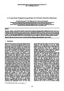
6. Numerical Examples In this section, some numerical examples are given to illustrate the availability of the two new models. Examples 1–3 consider the case in which there are 10 or 30 securities from different industries. Let 𝜉𝑖 be the return of the 𝑖th security determined as 𝜉𝑖 = (𝑝𝑖󸀠 + 𝑓𝑖 − 𝑝𝑖 )/𝑝𝑖 , where 𝑝𝑖󸀠 is the estimated closing price of the 𝑖th security in the next period, 𝑝𝑖 the closing price of the 𝑖th security at present, and 𝑓𝑖 the estimated dividends of the 𝑖th security during the next period. It is clear that 𝑝𝑖󸀠 and 𝑓𝑖 are unknown at present. In other words, the predictions of security returns have to be given mainly based on expert’s judgments and estimations. Example 1. Assume that each security return is the symmetrical triangular fuzzy variable denoted by 𝜉𝑖 = (𝑎𝑖 , 𝑏𝑖 , 𝑐𝑖 ) (𝑖 = 1, 2, . . . , 10), where the parameters 𝑎𝑖 , 𝑏𝑖 , and 𝑐𝑖 are determined based on the estimated values of financial experts. The data set is given in Table 1. Suppose that the minimum expected return the investor can accept is 1.95 and the bearable maximum risk is 1.0. In addition, the prior fuzzy investment return is 𝜂 = (−0.2, 1.9, 4.0). From the model (25), we can obtain a simple and crisp optimization model and employ fmincon in MATLAB 7.1 to solve this model. The numerical results are given in Table 2. In order to obtain the minimized distance of the investment return from 𝜂 when the portfolio satisfies the return and risk constraints, the investor should allocate his or her money according to Table 2. The corresponding objective value is 0.0150; the expected return and variance of the portfolio are 1.951 and 0.739, respectively. Furthermore, the investment return is 𝜉 = (−0.15, 1.95, 4.05). The graphic comparison of

8

Mathematical Problems in Engineering Table 2: Investment proportion of 10 securities (%).

Security 𝑖 Allocation of money

1 0.3

2 2.9

3 47.9

4 0.6

5 0.2

6 26.7

7 0.5

8 20.1

9 0.3

10 0.6

Table 3: The asymmetrical fuzzy returns of 10 securities. Security 𝑖 1

Fuzzy return 𝜉𝑖 (−0.4, 2.7, 3.4)

Security 𝑖 2

Fuzzy return 𝜉𝑖 (−0.1, 1.9, 2.6)

3

(−0.2, 3.0, 4.0)

4

(−0.5, 2.0, 2.9)

5

(−0.6, 2.2, 3.3)

6

(−0.1, 2.5, 3.6)

7

(−0.3, 2.4, 3.5)

8

(−0.1, 3.3, 4.5)

9

(−0.7, 1.1, 2.7)

10

(−0.2, 2.1, 3.8)

Table 4: Investment proportion of 10 securities (%). Security 𝑖 Allocation of money

1 0

2 0.4

3 6.8

4 0

5 1.6

6 0

7 0

8 35.2

9 1.2

10 54.9

Table 5: The trapezoidal fuzzy returns of 30 securities. Security 𝑖 1

Fuzzy return 𝜉𝑖 (1.000, 1.003, 1.007, 1.008)

Security 𝑖 2

Fuzzy return 𝜉𝑖 (1.001, 1.004, 1.009, 1.012)

3

(1.001, 1.004, 1.009, 1.012)

4

(0.996, 1.008, 1.009, 1.022)

5

(0.995, 1.007, 1.012, 1.023)

6

(0.994, 1.015, 1.024, 1.026)

7

(0.999, 1.019, 1.023, 1.038)

8

(1.005, 1.026, 1.032, 1.046)

9

(1.008, 1.021, 1.035, 1.046)

10

(1.017, 1.020, 1.026, 1.060)

11

(1.010, 1.027, 1.038, 1.055)

12

(1.013, 1.033, 1.045, 1.058)

13

(1.011, 1.039, 1.044, 1.062)

14

(1.015, 1.030, 1.044, 1.071)

15

(1.037, 1.053, 1.084, 1.096)

16

(1.042, 1.047, 1.070, 1.113)

17

(1.034, 1.055, 1.088, 1.100)

18

(1.039, 1.051, 1.088, 1.105)

19

(1.031, 1.067, 1.091, 1.108)

20

(1.048, 1.061, 1.067, 1.135)

21

(1.020, 1.089, 1.095, 1.107)

22

(1.043, 1.063, 1.092, 1.121)

23

(1.038, 1.073, 1.078, 1.132)

24

(1.051, 1.063, 1.104, 1.124)

25

(1.044, 1.076, 1.095, 1.134)

26

(1.039, 1.088, 1.097, 1.139)

27

(1.036, 1.089, 1.114, 1.127)

28

(1.054, 1.076, 1.089, 1.155)

29

(1.058, 1.070, 1.101, 1.150)

30

(1.056, 1.071, 1.126, 1.132)

the obtained investment return 𝜉 and the prior one 𝜂 is shown in Figure 1. From Figure 1, we see that the obtained investment return 𝜉 is close to the prior one 𝜂. It shows that the new approach is feasible. Example 2. In this example, all data is from [27]. The asymmetrical fuzzy returns of 10 securities are shown in Table 3. The maximum risk level and the minimum return level are 0.7 and 2.25, respectively. The prior fuzzy return is 𝜂 = (−0.2, 2.3, 4). From the model (30), we can obtain a simple and crisp optimization model and employ fmincon in MATLAB 7.1 to solve this model. The numerical results are given in Table 4.

In order to obtain the minimized distance of the investment return from the prior return 𝜂 when the portfolio satisfies the return and risk constraints, the investor should assign his or her capital according to Table 4. The corresponding objective value is 0.165; the expected return and semivariance of the portfolio are 2.253 and 0.612, respectively. In addition, the investment return is 𝜉 = (−0.18, 2.58, 4.03). 𝜁 = (−0.20, 2.63, 3.95) denotes the investment return calculated by [27]. The graphic comparison of the investment returns 𝜉, 𝜁 and the prior one 𝜂 is shown in Figure 2. From Figure 2, we can see that the investment returns obtained by our model and model of [27] are similar. However, solving our model is easier than solving the model of [27].

Mathematical Problems in Engineering

9

1

𝜇(x)

0.8 0.6 0.4 0.2 0 −0.20

0.5

1

1.5

2

2.5

3

3.5

4

x Prior investment return 𝜂 Investment return 𝜉

𝜇(x)

Figure 1: Comparison of investment return 𝜉 and the prior one 𝜂.

1 0.8 0.6 0.4 0.2 0 −0.20

0.5

1

1.5

2

2.5

3

3.5

4

x Prior investment return 𝜂 Investment return 𝜉 Investment return 𝜁

Figure 2: Comparison of the investment returns 𝜉, 𝜁 and the prior one 𝜂.

Table 6: Investment proportion of 30 securities (%). Security 𝑖 Allocation of money

14 10.17

18 0.12

23 4.9

26 33.01

27 17.85

28 0.23

29 33.69

Table 7: Investment proportion of 30 securities under different risk level constraints with 𝛼 = 1.0732 (%). 𝛽 Obj. 𝑥1 𝑥2 𝑥9 𝑥10 𝑥13 𝑥14 𝑥18 𝑥19 𝑥20 𝑥21 𝑥22 𝑥23 𝑥25 𝑥26 𝑥27 𝑥28 𝑥29 𝑥30

0.000245 0.0012 19.01 1.08 0 4.02 0 0 0 0 0 0 0 0 0 0 0 0 0 75.88

0.000255 9.7681𝑒 − 004 5.45 2.62 0.61 17.96 0.8 0 0 0 0 0 0 0 0 0 0 0 0 72.55

0.000265 4.7702𝑒 − 004 3.25 0.64 0 12.63 0.11 0 0 0 0 0 0 0 0 32.94 0 0 0 50.43

0.000275 1.6635𝑒 − 004 3.16 1.10 0 11.91 0 0 0 0 0 0 0 0 0 26.41 0 32.16 1.49 23.76

0.000315 1.5111𝑒 − 005 0 0 0 0.61 0 2.44 1.12 1.30 3.67 0 0.40 30.63 1.11 29.73 1.45 0.63 9.98 16.91

0.000345 1.3800𝑒 − 005 0 0 0 0.50 0 1.87 0.35 10.83 0 22.29 0.50 1.79 0.32 22.44 1.53 0.18 36.48 0.91

0.000475 9.7857𝑒 − 006 0 0 0 0 0 10.17 0.12 0 0 0 0 4.9 0 33.01 17.85 0.23 33.69 0

10

Mathematical Problems in Engineering Table 8: Investment proportion of 30 securities under different return level constraints with 𝛽 = 0.000475 (%).

𝛼 Obj. 𝑥14 𝑥16 𝑥18 𝑥19 𝑥20 𝑥21 𝑥22 𝑥23 𝑥25 𝑥26 𝑥27 𝑥28 𝑥29 𝑥30

1.0732 9.7857𝑒 − 006 10.17 0 0.12 0 0 0 0 4.9 0 33.01 17.85 0.23 33.69 0

1.0865 1.0206𝑒 − 005 4.9 0 0 8.53 0 0 0 16.17 0 20.37 17.74 1.51 30.65 0.14

1.0885 3.7685𝑒 − 005 0.48 0.14 0.17 0.32 14.92 8.98 0 3.63 0.23 20.5 17.15 0 18.06 15.4

1.0898 1.5338𝑒 − 004 0.38 0.40 0 0 17.33 0.46 1.0 1.51 2.43 20.14 26.63 0 0 29.73

1.919 2.0983𝑒 − 004 0.23 0 0 0 1.35 0 0 0.41 1.38 55.28 0 10.2 0 31.16

1.0953 4.6784𝑒 − 004 1.40 0 0 0 2.15 0.49 0 0 0 4.25 0 19.29 0 72.42

1.0962 0.0011 0 0 0 0 0 0 0 0 0 0 0 0.11 0 99.89

Table 9: Optimal portfolios produced by model (23) of [29] under different risk level constraints (%). 𝑠0 𝑥1 𝑥2 𝑥3 𝑥4 𝑥5 𝑥30

0.002 93.34 3.46 0 0 0 3.18

0.0025 92.49 0.14 0 0 0 7.36

0.0045 79.11 0.06 0 0 0 20.83

Example 3. Assume that each security return is trapezoidal fuzzy variable denoted by 𝜉𝑖 = (𝑎𝑖 , 𝑏𝑖 , 𝑐𝑖 , 𝑑𝑖 ) (𝑖 = 1, 2, . . . , 30). The data set from [30] is shown in Table 5. The maximum risk level and the minimum return level are 0.000475 and 1.0732, respectively. In addition, the prior fuzzy return is 𝜂 = (1.040, 1.075, 1.095, 1.135) for an investor. From the model (34), we can obtain a simple and crisp optimization model and use gravitation search algorithm (GSA) [42] to solve this model. The numerical results are given in Table 6. The results show that among 30 securities, satisfying the constraints, in order to minimize distance of the investment return from the prior return 𝜂, the investor should allocate his or her money according to Table 6. The corresponding objective value is 9.7857𝑒 − 006. In addition, the investment return is 𝜉 = (1.0424, 1.0754, 1.0950, 1.1333). In order to examine the sensitivity of the predetermined confidence level, we adjust the 𝛽 value and do the experiment. The results are shown in Table 7. It is seen that as maximum risk level increases, the optimal objective will decrease. In addition, we also examine the sensitivity of the return level 𝛼 to optimal objective in the same way. The results are given in Table 8. The results indicate that as expected return level increases, the minimal distance will increase. Furthermore, in order to examine the availability of the new approach, we compare the proposed method with the methods of [29, 30]. Based on the data in Table 5, we use GSA

0.0050 74.8 0.52 0.45 0.88 0 23.34

0.0075 58.37 0.74 0.29 0 0.35 40.24

0.0095 44.54 1.44 0 0.32 0 53.68

0.0125 21.99 3.87 0.34 0 0 73.75

to solve the models (18) and (23) of [29] for different return level 𝑟0 and risk level 𝑠0 . The numerical results are given in Tables 9 and 10. In addition, Tables 11 and 12 show the results of models (21) and (22) of [30], which are from [30]. From Tables 7 to 12, it is seen that the computational results about optimal allocation proportion to 30 securities are different, and the optimal portfolios produced by our model are more diversified than the optimal portfolio produced by models of [29, 30].

7. Conclusions In this paper, a concept of distance between fuzzy variables was introduced for measuring the divergence of fuzzy investment returns from a prior one. By defining the risk as variance and semivariance, two distance minimization models were proposed. In addition, crisp equivalents of the optimization models have also been provided. Finally, the results of the numerical examples illustrated the availability of the new method.

Conflict of Interests The authors declare that there is no conflict of interests regarding the publication of this paper.

Mathematical Problems in Engineering

11

Table 10: Optimal portfolios produced by model (18) of [29] under different return level constraints (%). 𝑟0 𝑥1 𝑥2 𝑥20 𝑥21 𝑥25 𝑥26 𝑥28 𝑥30

1.0732 6.69 1.64 61.01 30.6 0 0 0 0

1.0885 0 0 13.96 1.73 2.83 80.78 0 0

1.0898 0 0 3.13 3.75 0.14 92.65 0 0

1.0919 0 0 0 0 1.52 75.03 0 23.44

1.0953 0 0 2.83 0.61 0 0 8.4 88.06

1.0962 0 0 0 0 0 0 1.34 98.66

Table 11: Optimal portfolios produced by model (21) of [30] under different risk level constraints (%). 𝜑 𝑥1 𝑥15 𝑥20 𝑥21 𝑥26 𝑥28 𝑥30

0.000025 91.326 0 6.045 2.629 0 0 0

0.000475 11.338 44.196 24.411 20.055 0 0 0

0.000654 0 27.026 33.617 28.889 0 0 10.469

0.000779 0 0 34.866 28.094 8.539 0 28.501

0.000858 0 0 20.38 10.128 40.933 0 28.56

0.000932 0 0 3.097 0 62.456 4.976 29.471

0.000989 0 0 0 0 9.515 36.367 54.118

Table 12: Optimal portfolios produced by model (22) of [30] under different return level constraints (%). 𝜌 𝑥1 𝑥15 𝑥20 𝑥21 𝑥26 𝑥28 𝑥30

1.0732 0 44.39 29.887 25.732 0 0 0

1.0898 0 0 15.421 3.979 52.021 0 28.58

1.0919 0 0 4.392 0 62.61 3.419 29.58

Acknowledgments This work is partly supported by the National Natural Science Foundation of China (11371071) and Scientific Research Foundation of Liaoning Province Educational Department (L2013426).

References [1] H. markowitz, “Portfolio selection,” Journal of Finance, vol. 7, pp. 77–91, 1952. [2] A. Perold, “Large-scale portfolio optimization,” Management Science, vol. 30, pp. 1143–1160, 1984. [3] Y. Xia, B. Liu, S. Wang, and K. K. Lai, “A model for portfolio selection with order of expected returns,” Computers and Operations Research, vol. 27, no. 5, pp. 409–422, 2000. [4] Y. Crama and M. Schyns, “Simulated annealing for complex portfolio selection problems,” European Journal of Operational Research, vol. 150, no. 3, pp. 546–571, 2003. [5] X.-T. Deng, Z.-F. Li, and S.-Y. Wang, “A minimax portfolio selection strategy with equilibrium,” European Journal of Operational Research, vol. 166, no. 1, pp. 278–292, 2005.

1.0953 0 0 0 0 0 34.545 65.454

1.0962 0 0 0 0 0 1.818 98.182

1.09625 0 0 0 0 0 0 100

[6] H. Markowitz, P. Todd, G. Xu, and Y. Yamane, “Computation of mean-semivariance efficient sets by the critical line algorithm,” Annals of Operations Research, vol. 45, no. 1, pp. 307–317, 1993. [7] B. Rom and K. Ferguson, “Post-modern portfolio theory comes of age,” Journal of Investing, vol. 3, pp. 11–17, 1994. [8] K. Chow and K. Denning, “On variance and lower partial moment betas: the equivalence of systematic risk measures,” Journal of Business Finance and Accounting, vol. 21, pp. 231–241, 1994. [9] H. Grootveld and W. Hallerbach, “Variance vs downside risk: is there really that much difference?” European Journal of Operational Research, vol. 114, no. 2, pp. 304–319, 1999. [10] G. Homaifar and D. Graddy, “Variance and lower partial moment betas as alternative risk measures in cost of capital estimation: a defense of the CAPM beta,” Journal of Business Finance and Accounting, vol. 17, pp. 677–688, 1990. [11] J. Kapur and H. Kesavan, Entropy Optimization Principles with Applications, Academic Press, New York, NY, USA, 1992. [12] A. S. Cherny and V. P. Maslov, “On minimization and maximization of entropy in various disciplines,” Theory of Probability and Its Applications, vol. 48, no. 3, pp. 447–464, 2004.

12 [13] S. Fang, J. Rajasekera, and H. Tsao, Entropy Optimization and Mathematical Programming, Kluwer Academic, Boston, Mass, USA, 1997. [14] R. Rubinstein, “Semi-iterative minimum cross-entropy algorithms for rare-events, counting, combinatorial and integer programming,” Methodology and Computing in Applied Probability, vol. 10, no. 2, pp. 121–178, 2008. [15] M. R. Simonelli, “Indeterminacy in portfolio selection,” European Journal of Operational Research, vol. 163, no. 1, pp. 170–176, 2005. [16] A. Bilbao-Terol, B. P´erez-Gladish, M. Arenas-Parra, and M. V. Rodr´ıguez-Ur´ıa, “Fuzzy compromise programming for portfolio selection,” Applied Mathematics and Computation, vol. 173, no. 1, pp. 251–264, 2006. [17] P. Gupta, M. K. Mehlawat, and A. Saxena, “Asset portfolio optimization using fuzzy mathematical programming,” Information Sciences, vol. 178, no. 6, pp. 1734–1755, 2008. [18] X. Zhang, W.-G. Zhang, and W.-J. Xu, “An optimization model of the portfolio adjusting problem with fuzzy return and a SMO algorithm,” Expert Systems with Applications, vol. 38, no. 4, pp. 3069–3074, 2011. [19] X. Huang, “Portfolio selection with fuzzy returns,” Journal of Intelligent and Fuzzy Systems, vol. 18, no. 4, pp. 383–390, 2007. [20] X. Huang, “Mean-semivariance models for fuzzy portfolio selection,” Journal of Computational and Applied Mathematics, vol. 217, no. 1, pp. 1–8, 2008. [21] X. Li, Z. Qin, and S. Kar, “Mean-variance-skewness model for portfolio selection with fuzzy returns,” European Journal of Operational Research, vol. 202, no. 1, pp. 239–247, 2010. [22] R. Bhattacharyya, S. Kar, and D. D. Majumder, “Fuzzy meanvariance-skewness portfolio selection models by interval analysis,” Computers and Mathematics with Applications, vol. 61, no. 1, pp. 126–137, 2011. [23] X. Huang, “An entropy method for diversified fuzzy portfolio selection,” International Journal of Fuzzy Systems, vol. 14, no. 1, pp. 160–165, 2012. [24] P. Li and B. Liu, “Entropy of credibility distributions for fuzzy variables,” IEEE Transactions on Fuzzy Systems, vol. 16, no. 1, pp. 123–129, 2008. [25] X. Huang, “Mean-entropy models for fuzzy portfolio selection,” IEEE Transactions on Fuzzy Systems, vol. 16, no. 4, pp. 1096–1101, 2008. [26] X. Li and B. Liu, “Fuzzy cross-entropy and its applications,” Tech. Rep., 2007. [27] Z. Qin, X. Li, and X. Ji, “Portfolio selection based on fuzzy crossentropy,” Journal of Computational and Applied Mathematics, vol. 228, no. 1, pp. 139–149, 2009. [28] W. Tang, X. Li, and R. Zhao, “Metric spaces of fuzzy variables,” Computers and Industrial Engineering, vol. 57, no. 4, pp. 1268– 1273, 2009. [29] Y. Chen, Y. Liu, and X. Wu, “A new risk criterion in fuzzy environment and its application,” Applied Mathematical Modelling, vol. 36, no. 7, pp. 3007–3028, 2012. [30] X.-L. Wu and Y.-K. Liu, “Spread of fuzzy variable and expectation-spread model for fuzzy portfolio optimization problem,” Journal of Applied Mathematics and Computing, vol. 36, no. 1-2, pp. 373–400, 2011. [31] L. A. Zadeh, “Fuzzy sets,” Information and Control, vol. 8, no. 3, pp. 338–353, 1965. [32] L. A. Zadeh, “Fuzzy sets as a basis for a theory of possibility,” Fuzzy Sets and Systems, vol. 1, no. 1, pp. 3–28, 1978.

Mathematical Problems in Engineering [33] D. Dubois and H. Prade, Possibility Theory: An Approach to Computerized Processing of Uncertainty, Plenum Press, New York, NY, USA, 1988. [34] D. Dubois and H. Prade, “Fuzzy numbers: an overview,” Analysis of Fuzzy Information, vol. 2, pp. 3–39, 1988. [35] B. Liu and Y.-K. Liu, “Expected value of fuzzy variable and fuzzy expected value models,” IEEE Transactions on Fuzzy Systems, vol. 10, no. 4, pp. 445–450, 2002. [36] B. Liu, Uncertainty Theory, Springer, Berlin, Germany, 2nd edition, 2007. [37] B. Liu, “A survey of credibility theory,” Fuzzy Optimization and Decision Making, vol. 5, no. 4, pp. 387–408, 2006. [38] B. Liu, “A survey of entropy of fuzzy variables,” Journal of Uncertain Systems, vol. 1, pp. 4–13, 2007. [39] R. E. Moore, Method and Application of Interval Analysis, SIAM, Philadelphia, Pa, USA, 1979. [40] X. Zhang and P. Liu, “Method for multiple attribute decisionmaking under risk with interval numbers,” International Journal of Fuzzy Systems, vol. 12, no. 3, pp. 237–242, 2010. [41] P. Chunhachinda, K. Dandapani, S. Hamid, and A. J. Prakash, “Portfolio selection and skewness: evidence from international stock market,” Journal of Banking and Finance, vol. 21, pp. 143– 167, 1997. [42] E. Rashedi, H. Nezamabadi-pour, and S. Saryazdi, “GSA: a gravitational search algorithm,” Information Sciences, vol. 179, no. 13, pp. 2232–2248, 2009.

Advances in

Operations Research Hindawi Publishing Corporation http://www.hindawi.com

Volume 2014

Advances in

Decision Sciences Hindawi Publishing Corporation http://www.hindawi.com

Volume 2014

Journal of

Applied Mathematics

Algebra

Hindawi Publishing Corporation http://www.hindawi.com

Hindawi Publishing Corporation http://www.hindawi.com

Volume 2014

Journal of

Probability and Statistics Volume 2014

The Scientific World Journal Hindawi Publishing Corporation http://www.hindawi.com

Hindawi Publishing Corporation http://www.hindawi.com

Volume 2014

International Journal of

Differential Equations Hindawi Publishing Corporation http://www.hindawi.com

Volume 2014

Volume 2014

Submit your manuscripts at http://www.hindawi.com International Journal of

Advances in

Combinatorics Hindawi Publishing Corporation http://www.hindawi.com

Mathematical Physics Hindawi Publishing Corporation http://www.hindawi.com

Volume 2014

Journal of

Complex Analysis Hindawi Publishing Corporation http://www.hindawi.com

Volume 2014

International Journal of Mathematics and Mathematical Sciences

Mathematical Problems in Engineering

Journal of

Mathematics Hindawi Publishing Corporation http://www.hindawi.com

Volume 2014

Hindawi Publishing Corporation http://www.hindawi.com

Volume 2014

Volume 2014

Hindawi Publishing Corporation http://www.hindawi.com

Volume 2014

Discrete Mathematics

Journal of

Volume 2014

Hindawi Publishing Corporation http://www.hindawi.com

Discrete Dynamics in Nature and Society

Journal of

Function Spaces Hindawi Publishing Corporation http://www.hindawi.com

Abstract and Applied Analysis

Volume 2014

Hindawi Publishing Corporation http://www.hindawi.com

Volume 2014

Hindawi Publishing Corporation http://www.hindawi.com

Volume 2014

International Journal of

Journal of

Stochastic Analysis

Optimization

Hindawi Publishing Corporation http://www.hindawi.com

Hindawi Publishing Corporation http://www.hindawi.com

Volume 2014

Volume 2014