Position control of a robotic manipulator using neural network ... - wseas

7th WSEAS Int. Conf. on ARTIFICIAL INTELLIGENCE, KNOWLEDGE ENGINEERING and DATA BASES (AIKED'08), University of Cambridge, UK, Feb 20-22, 2008

Position Control of a Robotic Manipulator Using Neural Network and a Simple Vision System Bach H. Dinh, Matthew W. Dunnigan, Donald S. Reay Electrical, Electronic & Computer Engineering School of Engineering and Physical Sciences Heriot-Watt University EH14 4AS Edinburgh, UK Abstract : This paper describes a new approach for approximating the inverse kinematics of a manipulator using a RBFN (Radial Basis Function Network). In fact, there are several traditional methods based on the known geometry of the manipulator to calculate the relationship between the joint variable space and the world coordinate space. However, these traditional methods are impractical if the manipulator geometry cannot be determined, in a robot-vision system for example. Therefore, a neural network with its inherent learning ability can be an effective alternative solution for the inverse kinematics problem. In this paper, a training solution using the strict interpolation method and the LMS (Least Mean Square) algorithm is presented in a two phase training procedure. The strict interpolation method with regularly-spaced-position training patterns in the workspace can produce an appropriate approximation of the inverse kinematic function. However, this solution has the main difficulty in how to collect accurate training patterns whose inputs are selected at pre-defined positions in the workspace. Additionally, the LMS algorithm can improve the approximate function iteratively through on-line training with arbitrary position patterns. A training approach combining two mentioned techniques can be applied for the inverse kinematics problem even with an inaccurate training set. It consists of two steps, firstly producing an inaccurate inverse kinematic approximation by strict interpolation (reflecting the situation that the initial setup and application environments are different) and then re-correcting the network through on-line training by the LMS. The advantages of both training methods can deal with the difficulty of collecting training patterns for practical applications. To verify the performance of the proposed approach, a practical experiment has been performed using a Mitsubishi PA10-6CE manipulator observed by a webcam. All application programmes, such as robot servo control, neural network, and image processing were written in C/C++ and run in a real robotic system. The experimental results prove that the proposed approach is effective. Keywords: RBFN, robot-vision, training approach, inverse kinematics, PA10-6CE manipulator.

1 Introduction In robot kinematics there are two important problems, forward and inverse kinematics. Forward kinematics can be regarded as a one-to-one mapping from the joint variable space to the Cartesian coordinate space (world space). From a set of joint angles, forward kinematics determines the corresponding location (position and orientation) of the end-effector. This problem can be easily solved by the 4x4 homogenous transformation matrices using the Denavit & Hartenbergh representation [1]. Inverse kinematics is used to compute the corresponding joint angles from location of the endeffector in space. Obviously, inverse kinematics is a more difficult problem than forward kinematics because of its multi-mapping characteristic. There are many solutions to solve the inverse kinematics problem, such as the geometric, algebraic, and numerical iterative methods. In particular, some of

ISSN: 1790-5109

the most popular methods are mainly based on inversion of the mapping established between the joint space and the task space by the Jacobian matrix [2]. This solution uses numerical iteration to invert the forward kinematic Jacobian matrix and does not always guarantee to produce all the possible inverse kinematic solutions and involves significant computation. In cases where the manipulator geometry cannot be exactly specified, the traditional methods become very difficult or impossible, for example the robot-vision system. The artificial neural network, which has significant flexibility and learning ability, has been used in many robot control problems. In fact, for the inverse kinematics problem several neural network architectures have been used, such as MLPN (MultiLayer Perceptron Network), Kohonen selforganizing map and RBFN. In [3][4] Guez et al and Choi described solutions using the MLPN and back

Page 232

ISBN: 978-960-6766-41-1


propagation training algorithm. Additionally, Watanabe in [5] determined optimal numbers of neurons in a MLPN for approximating the inverse kinematic function. To deal with complex manipulator structures some particular neural network architectures were presented, for example a combination between the MLPN and the look-up table [6]. A modular neural network in which the modules were concatenated in a global scheme in order to perform the inverse kinematics in a sequential way was proposed by Pablo [7]. Similarly, in [8][9][10] the inverse kinematic approximation using a RBFN was presented to compare with the performance of the MLPN. However, most of these mentioned methods used the inverse function of the forward kinematic transformation to build the mapping from world coordinate space to joint angle space. It means that the manipulator geometry or the forward kinematics must be known to collect the training patterns for the neural networks. However, with a robot-vision system the position of the robot is just observed via a camera, so the manipulator geometry is not required. In this paper, the position of the manipulator in the workspace is represented by image coordinates instead of world coordinates. Therefore, the RBFN can learn an indirect inverse kinematic function of the manipulator observed by the camera to control its movement in the workspace without any knowledge of the manipulator geometry or forward kinematics. Since this data can be easily determined by simple visual measurement it is convenient for practical applications such as remote robot control. This solution is known as an image-based control scheme. In this paper two training methods, strict interpolation and LMS, were applied to train the RBFN. Training the RBFN using strict interpolation with regularly spaced position patterns represents a different idea from other existing papers [8][9][10]. It is possible to determine an appropriate approximation of the inverse kinematic function. However, this solution has a main difficulty in how to collect the accurate training patterns whose inputs are selected at pre-defined positions in the workspace of a real robotic system. Additionally, using the LMS to update the linear weights can improve the RBFN performance through on-line training. Therefore, the combination of strict interpolation and LMS methods produces the advantages of both training methods to deal with the difficulty in collecting training patterns in practical applications. This approach consists of two steps, firstly producing an inaccurate inverse kinematic approximation by strict interpolation and then re-

ISSN: 1790-5109

correcting it through on-line training by the LMS. The approximation is inaccurate reflecting the reasonable assumption that the initial network training occurs in an environment that is not exactly the same as the environment where the system is actually deployed. In theory, this approach is a different idea from others in which neural network should be learn directly from accurate input-output patterns. The principle of the presented approach is that neural network should be pre-trained from an easy and feasible case but less accurate and then improved through on-line correction according to its adaptive ability. The paper is organized as follows. The first section has introduced the basis ideas and background of the inverse kinematics problem using neural networks. In the second section, the approach using the RBFN to approximate the manipulator inverse kinematics is presented. It describes the RBFN architecture and presents the training methods to learn the inverse kinematic function. The practical experiment and results are described in the next section that verify the proposed approach. Finally, the main conclusions are outlined in the last section.

2 Inverse Kinematics Approximation Using A Radial Basis Function Network The basic architecture of a RBFN is the three layer network consisting of input layer, hidden layer and linear output layer [11]. In the inverse kinematics problem, the inputs and outputs of the RBFN are position (image coordinates) and joint angles of the manipulator respectively. The unique feature of the RBFN compared to the MLP and other networks is the process performed at the hidden layer. In this hidden layer, the radial basis function works as a local selector in which the corresponding output depends on the distance between its centre and input. It can be presented as: ⎛ x − ci Φ i ( x) = exp⎜ − ⎜ σ2 ⎝ ri =

2 ⎛ ⎞ ⎟ = exp⎜ − ri ⎟ ⎜ σ2 ⎠ ⎝

⎞ ⎟ ⎟ ⎠

K

∑ ( x k − c ki ) 2

(1)

(2)

k =1

where Фi – Radial basis function (Gaussian function) ci – centre of the i-th hidden unit (i = 1, 2,…, I) σ - width of the Gaussian function ri - distance between input and centre of the i-th hidden unit

Page 233

ISBN: 978-960-6766-41-1


x – input of the RBFN (k = 1, 2,…, K) then, the outputs of the RBFN are expressed as : M

y j ( x) = ∑ W ji Φ i ( x)

linear weights can be modified by the simple expression below: (6) ΔW ji = η .e j .Φ i

(3)

i =1

e j = Tj − y j

Wji – synaptic weight between the i-th hidden unit and the j-th output yj – the j-th output of the RBFN- joint angle (j = 1, 2,.., J) One of the simplest ways to train the RBFN is to select training patterns as inputs which coincide with the centres of hidden units and calculate the linear weights based on the interpolation method. This is called the strict interpolation method [11] where the RBFN is an exact mapping of all observations in the training data set. Given a training data set, consisting of N inputs different positions in the workspace, and N targets corresponding manipulator joint angles: {(X1, X2, .., XN); (T1, T2, …, TN)}, these known data points Xi are taken to be the centres Ci of the hidden units. Then, after all training patterns have been presented to the RBFN, the NxN matrix called the interpolation matrix can be obtained as: ⎡ Φ1 (1) Φ 2 (1) ⎢ Φ (2) Φ (2) 2 Φ=⎢ 1 ⎢ # # ⎢ ⎣ Φ1 ( N ) Φ 2 ( N )

" Φ N (1) ⎤ " Φ N (2) ⎥⎥ % # ⎥ ⎥ " Φ N ( N )⎦

(4)

The linear weights are calculated from the targets and the interpolation matrix from the following equation: W = T .Φ −1 (5) This solution is an exact mapping f : Xi Æ Ti (i = 1,2,…N), for all patterns presented to the RBFN and its generalization is dependent on the appropriate selection of the hidden layer structure (centres of hidden units and width of Gaussian function). This is an off-line training process with known training patterns. In this paper, the RBFN and the strict interpolation method are used with the inputs of training patterns (centres of hidden layer) uniformly distributed in the workspace in order to produce an inverse kinematic approximation from a small number of hidden units. The second approach called the LMS (Least Mean Square) method is more general than the former and can be applied for on-line training. In this approach, centres of the hidden layer are not taken from the inputs of the training patterns but have been predefined already and the linear weights are incrementally updated when a training pattern is presented to the network. As described in [11], the

ISSN: 1790-5109

where ej - error between target and actual output j η – learning rate. In fact, the difficulty of using the strict interpolation method in the inverse kinematics problem is how to collect patterns in which their inputs are uniformly distributed in the workspace. It means that centres of the hidden layer should be put at pre-defined positions and then the joint angles must be determined correspondingly without any known inverse kinematics. This kind of data is called the regularly spaced position training pattern. In real robotic systems, it can only be estimated by experiment with an undetermined accuracy and also needs many attempts depending on the system’s complexity. Therefore, there should be a compromise between the accuracy and the complexity of the training solution. The principle of the presented approach is that neural network should be pre-trained from an easy and feasible case which produces an initially approximate model and then is improved through on-line correction according to its adaptive ability. On the other hand, collecting an arbitrary position pattern is much easier than collecting a constrained pattern as above. Hence, all of the existing approaches [8][9][10] used this arbitrary data to train the RBFN. In this paper, the training patterns for on-line training using the LMS method were collected by arbitrarily moving the manipulator in the workspace. An approach combining the strict interpolation and the LMS method is applied to solve the inverse kinematics of a simple robot-vision system.

3 Practical Work and Discussion Practical experiments have been developed and performed using the existing facilities in the Intelligent Robotics Laboratory [12]. The following elements of the system can be identified: • The Mitsubishi PA10-6CE manipulator with servo controller. This is the six link multipurpose arm connected to an industrial PC (IPC) via an ARC-Net interface. • The IPC running under the QNX Neutrino real-time operating system is used to execute control programmes and communicate with an application PC (APC) via Internet interface.

Page 234

ISBN: 978-960-6766-41-1


•

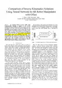
A standard webcam mounted on a vertical shaft that permits rotation captures the manipulator images in two dimensional space. • All of the main application programmes were written in C/C++ and run in the APC. Fig.1 presents a simple robot-vision system, consisting of the PA10-6CE manipulator and the webcam. y IMAGE COORDINATE SYSTEM

LED WORLD COORDINATE SYSTEM

WEBCAM

Z z

X

x

Fig.1 – Simple visual measurement system The webcam and an image processing programme developed from OpenCV library are used as the simple visual measurement where the relative position of the manipulator can be directly determined by two dimensional coordinates (x,y) in the image plane. Obviously, this can be performed without camera calibration or the manipulator geometry. In other words, the visual measurement system can directly determine the relative positions of any manipulator with unknown geometry in the image plane. Therefore, the inputs of the RBFN are image coordinates (x,y) instead of world coordinates (X,Y,Z) and the inverse kinematic function then is the mapping from image coordinates (x,y) to joint angles. However, this simple visual measurement is easily influenced due to variations in configured parameters of the robot-vision system. This sensitivity is common in practice. Fig.2 presents the general structure of the real robotic system used in this practical work. The PA10-6CE manipulator was controlled to move in two dimensional space by allowing movement only of the second and third joints (J2 and J3). Thus, the problem was to determine the inverse kinematics of a two link manipulator and this RBFN consisted of two inputs (x,y) and two outputs (J2,J3) correspondingly. In the working area of the manipulator, the centres of the hidden layer were uniformly distributed as a grid. The video frame at the resolution of 640x480 (pixels) was created and forwarded to the image processing programme to determine image coordinates (x,y) of the

ISSN: 1790-5109

manipulator. The experiment is carried out with the following steps: • Step 1 : A set of the regularly spaced position training patterns is manually collected in the workspace of the PA10-6CE manipulator. It is performed by the joint servo controller and the visual measurement. The quality or accuracy of collected data depends on the user’s observation and a poor pattern means that its input deviates from pre-defined position. This needs many attempts to obtain acceptable training data. • Step 2 : After collecting training data as above, a noise value +20 is added in the target outputs of the training patterns while the inputs are still unchanged to make a set of inaccurate training patterns. This reflects the fact that the set-up and actual application environments are different. • Step 3 : Using the inaccurate data to train the RBFN by the strict interpolation establishes an incorrect inverse kinematic function. It is the off-line training phase. • Step 4 : Step 4 is used to improve the existing RBFN through an on-line training phase. It can be briefly described as: - Moving the PA10-6CE manipulator to an arbitrary position and collecting the training pattern (image coordinates and corresponding joint angles) - Update the linear weights by the LMS algorithm according to the recent pattern. - Repeat until stop command sent.

Page 235

L.E.D (X,Y)

WEBCAM

IMAGE PROCESSING

J1

x y

Θ1 RBF

Θ2

ROBOT CONTROLLER

J2

(θ1, θ2) = I(x,y)

Fig.2 – General structure of experimental robotic system

ISBN: 978-960-6766-41-1


To verify the performance of the RBFN, a test data set was presented after each training phase. It is a position control task moving the PA10-6CE manipulator along the trajectory as shown in Fig.3, Fig.4, and Fig.5. An incorrect inverse kinematic function was built by the strict interpolation method with the inaccurate training patterns as described in step 2 and 3. Fig.3 presents the performance of the RBFN after trained by inaccurate data and the errors introduced are obvious from inspection. TARGET AND ACTUAL TRAJECTORY 350

TARGET TRAJECTORY ACTUAL TRAJECTORY

340

330

COOR DINATE Y (PIXEL)

320

310

300

290

280

In Fig.5 the performance of the RBFN after on-line training with 100 patterns is presented. As can be seen, the actual trajectory is close to the desired trajectory with an error of approximately 1 or 2 pixels (one pixel is equivalent to 2 mm). The performance is highly satisfactory because the quality of this robotic system is dependent not only on the RBFN learning ability but also the accuracy of the training data, quality of the visual measurement system, and even the precision of the servo controller. Moreover, the experimental results show that as the distance between the centres becomes smaller the better the generalization. In other words, the RBFN needs more hidden units to improve the accuracy of the inverse kinematic function. Obviously, there is a practical limit in the number of centres of the hidden layer due to lack of memory and complicated architecture of the network.

270

TARGET AND ACTUAL TRAJECTORY 350

260

TARGET TRAJECTORY ACTUAL TRAJECTORY

340 250

330 240 240

250

260

270

280

290

300

310

320

330

340

350

COORDINATE X (PIXEL)

320

To correct the existing function, an on-line training process was applied using the LMS algorithm as described in step 4. The linear weights are adjusted for each recent training pattern recorded from arbitrarily moving the PA10-6CE. After training by a number of training patterns, the RBFN was corrected incrementally and the performance of the robotic system was clearly improved. Fig.4 shows the performance of the RBFN after 10 on-line training patterns. TARGET AND ACTUAL TRAJECTORY 350 TARGET TRAJECTORY ACTUAL TRAJECTORY

340

330

C OORD INATE Y (PIXEL)

320

310

300

290

280

270

260

250

240 240

250

260

270

280

290

300

310

320

330

340


Fig.4 – Performance of the RBFN after on-line training with 10 arbitrary training patterns

ISSN: 1790-5109

350

C OOR D IN ATE Y (PIXEL)

Fig. 3 – Performance of the RBFN trained by inaccurate data

310

300

290

280

270

260

250

240 240

250

260

270

280

290

300

310

320

330

340

350


Fig.5 – Performance of the RBFN after on-line retraining with 100 arbitrary training patterns Since the RBFN acts as a locally tuned function, only hidden units close enough to the training pattern positions contribute noticeably to the network output. As a result, only the linear weights connected to these hidden units are adjusted via online training. It means that the positions of the training data have an important impact in the on-line training process. The closer the training pattern to the test points, the stronger the effect in modifying the linear weights of the RBFN in that area. Different patterns presented to the RBFN can produce different improvement effects in the approximate function. Thus, the distribution of training patterns should cover the entire workspace to modify the whole of the inverse kinematic function.

Page 236

ISBN: 978-960-6766-41-1


In general, it appears that the RBFN after on-line modifying is closer to the correct inverse kinematic function. In other words, the RBFN is improved through on-line training and can approach the accurate inverse kinematic function after a sufficient number of training epochs.

4 Conclusion A new approach for approximating the inverse kinematics without the manipulator geometry is proposed by using a RBFN and the combination of strict interpolation and LMS methods. The strict interpolation method with regularly spaced position training patterns can produce an appropriate approximation of the inverse kinematic function. However, this solution has a main difficulty in how to collect the accurate training patterns in the workspace of a real robotic system. Additionally, the LMS algorithm can improve the RBFN iteratively through on-line training with arbitrary patterns. Therefore, the combination of these techniques produces the advantages of both training methods to deal with the difficulty in practical applications. Practical work using the PA10-6CE manipulator observed by the webcam verified the proposed approach. References: [1] – K.S.Fu, R.C.Gonzalez, C.S.G.Lee. Robotics : Control, Sensing, Vision, and Intelligence. McGraw-Hill, 1987. [2] – W. Khalil and E. Dombre. Modeling, Identification, and Control of Robots. Hermes Penton, 2002. [3] – Benjamin B. Choi and Charles Lawrence. Inverse Kinematics Problem in Robotics Using Neural Networks. NASA Technical Memorandum, 105869. Oct.1992 [4] – Allon Guez, Ziauddin Ahmad. Solution to The Inverse Kinematics Problem in Robotics by Neural Networks. In Proceedings of the IEEE International

ISSN: 1790-5109

Conference on Neural Networks, Vol.1, pp.617-624. July, 24-27 1988. San Diego, California, USA. [5]- Eiji Watanabe and Hikaru Shimizu. A Study on Generalization Ability of Neural Network for Manipulator Inverse Kinematics. In Proceedings of the Seventeenth International Conference on Industrial Electronics, Control and Instrumentation, Vol.2, pp. 957-962. 28 Oct-1 Nov 1991. Kobe, Japan. [6] – A.S. Morris and A. Mansor. Finding the Inverse Kinematics of Manipulator Arm Using Artificial Neural Network with Lookup Table. Robotica (Cambridge University Press), Vol.15, pp. 617-625. 1997. [7] – Pablo J. Alsina, Narpat S. Gehlot. Robot Inverse Kinematics: A Modular Neural Network Approach. In Proceedings of 38th Midwest Symposium on Circuits and Systems, Vol.2, pp. 631634. August, 13-16 1995. Rio de Janeiro, Brazil. [8] – Pei-Yan Zhang, Tian Sheng Lu, Li Bo Song. RBF Networks-Based Inverse Kinematics of 6R Manipulator. The International Journal of Advanced Manufacturing Technology, Volume 26, 2004, pp. 144-147. Springer- Verlag London Ltd. [9] – S.S. Yang, M. Moghavvemi, and John D. Tolman. Modelling of Robot Inverse Kinematics Using Two ANN Paradigms. In Proceedings of TENCON2000-Intelligent System and Technologies for the New Millennium, Volume 3, pp. 173-177. September, 24-27 2000. Kuala Lumpur, Malaysia. [10] – Joseph A. Driscoll. Comparison of Neural Network Architectures for the Modelling of Robot Inverse Kinematics. In Proceedings of The IEEE SOUTHEASTCON 2000, Vol.3, pp. 44-51. April, 79 2000. Tennessee USA. [11] – Simon Haykin. Neural networks - A Comprehensive Foundation. Prentice Hall, Inc. 1999 [12]- Cyprian M. Wronka, Matthew W. Dunnigan. Internet Remote Control Interface for A Multipurpose Robotic Arm. The International Journal Of Advanced Robotic Systems. Volume 3, pp. 179-182. June 2006.

Page 237

ISBN: 978-960-6766-41-1