to generalizations of generators, such as disjunction-free sets and ... minimum support threshold, we call the itemset a frequent generator. ... hce:2, hd:2, hde:2, hcd:2 hcde:2, ie:2, ..... In Proc. of the 7th ICDT Conference, pages 398â. 416, 1999.
Positive Borders or Negative Borders: How to Make Lossless Generator Based Representations Concise Guimei Liu1,2
Jinyan Li1
Limsoon Wong2
Wynne Hsu2
1
2
Institute for Infocomm Research, Singapore School of Computing, National Univeristy of Singapore, Singapore
Abstract A complete set of frequent itemsets can get undesirably large due to redundancy. Several representations have been proposed to eliminate the redundancy. Existing generator based representations rely on a negative border to make the representation lossless. However, negative borders of generators are often very large. The number of itemsets on a negative border sometimes even exceeds the total number of frequent itemsets. In this paper, we propose to use a positive border together with frequent generators to form a lossless representation. A set of frequent generators plus its positive border is always no larger than the corresponding complete set of frequent itemsets, thus it is a true concise representation. The generalized form of this representation is also proposed. We develop an efficient algorithm, called GrGrowth, to mine generators and positive borders as well as their generalizations.
1
Introduction
Frequent itemset mining is an important problem in the data mining area. It was first introduced by Agrawal et al.[1] in the context of transactional databases. The number of frequent itemsets can be undesirably large, especially on dense datasets where long patterns are prolific. Many frequent itemsets are redundant because their support can be inferred from other frequent itemsets. Generating too many frequent itemsets not only requires extensive mining cost but also defeats the primary purpose of data mining in the first place. Several concepts have been proposed to eliminate the redundancy from a complete set of frequent itemsets, including frequent closed itemsets [12], generators [2] and generalizations of generators [4, 10]. In some applications, generators are more preferable than closed itemsets. For example, generators are more appropriate for classification than closed itemsets because closed itemsets contain some redundant items that are not useful for classification, which also violates the minimum description length principle. The redundant items sometimes have a negative impact on classification ac-
curacies because they can prevent a new instance from matching a frequent itemset. A representation is lossless if we can decide for any itemset whether it is frequent and we can determine the support of the itemset if it is frequent, using only information of the representation without accessing the original database. Generators alone are not adequate for representing a complete set of frequent itemsets. Existing generator based representations [4, 9, 10] use a negative border together with frequent generators to form a lossless representation. We have observed that negative borders are often very large, and sometimes the negative border alone is larger than the corresponding complete set of frequent itemsets. For example, the total number of frequent itemsets is 122450 in dataset BMS-POS with minimum support of 0.1%, while the number of itemsets on the negative border is 236912. To solve this problem, we propose a new concise representation of frequent itemsets, which uses a positive border together with generators to form a lossless representation. The main contributions of the paper are summarized as follows: (1) We propose a new concise representation of frequent itemsets, which uses a positive border instead of a negative border together with frequent generators to represent a complete set of frequent itemsets. The size of the new representation is guaranteed to be no larger than the total number of frequent itemsets, thus it is a true concise representation. Our experiment results show that a positive border is usually orders of magnitude smaller than its corresponding negative border. (2) The completeness of the new representation is proved, and an algorithm is given to derive the support of an itemset from the new representation. (3) We develop an efficient algorithm GrGrowth to mine frequent generators and positive borders. The GrGrowth algorithm and the concept of positive borders can be both applied to generalizations of generators, such as disjunction-free sets and generalized disjunction-free sets. The rest of the paper is organized as follows. Section 2 presents related work. The formal definitions
Copyright © by SIAM. Unauthorized reproduction of this article is prohibited
469
of positive border based representations are given in of I is called an itemset. The support of an itemset l in Section 3. Section 4 describes the mining algorithm. D is defined as support(l)=|{t|t ∈ D and l ⊆ t}|/|D| or The experiment results are shown in Section 5. support(l)=|{t|t ∈ D and l ⊆ t}| . 2 Related Work The problem of removing redundancy while preserving semantics has drawn much attention in the data mining area. Several concepts have been proposed to remove redundancy from a complete set of frequent itemsets, including frequent closed itemsets [12], generators [2] and generalizations of generators [4, 10, 5, 6, 3]. The concept of generators is first introduced by Bastide et al. [2]. Bykowski et al. [4] propose another concept—disjunction-free generator to further reduce result size. Generators or disjunction-free generators alone are not adequate to represent a complete set of frequent itemsets. Bykowski et al. use a negative border together with disjunction-free generators to form a lossless representation. Kryszkiewicz et al. [10] generalize the concept of disjunction-free generator and propose to mine generalized disjunction-free generators. Boulicaut et al. [3] generalize the generator representation from another direction and propose the δ-free-sets representation. Itemset l is δ-free if the support difference between l and l’s subsets is less than δ. Boulicaut et al. also use a negative border together with δ-freesets to form a concise representation. The δ-free-sets representation is not lossless unless δ=0. Mannila et al. [11] first propose the notion of condensed representation based on the inclusion-exclusion principle. Calders et al. [5] propose a similar concept— non-derivable frequent itemsets. An itemset is nonderivable if its support cannot be inferred from its subsets based on the inclusion-exclusion principle. Calders et al. develop a level-wise algorithm NDI [5] and a depth-first algorithm dfNDI [7] to mine non-derivable frequent itemsets. The dfNDI algorithm is shown to be much more efficient than the NDI algorithm. Calders et al. [6] also propose the concept of k-free sets and several types of borders to form lossless representations. However, the computation cost for inferring support from non-derivable itemsets and k-free sets is very high. 3 Positive Border Based Representations In this section, we first give the formal definitions of generators and positive borders, and then give an algorithm to infer the support of an itemset from positive border based representations. 3.1
Definitions Let I = {a1 , a2 , · · · , an } be a set of items and D = {t1 , t2 , · · · , tN } be a transaction database, where ti (i ∈ [1, N ]) is a transaction and ti ⊆ I. Each subset
Definition 3.1. (Generator) Itemset l is a generator if there does not exist l′ such that l′ ⊂ l and support(l′ ) = support(l). According to the definition, the empty set φ is a generator in any database. If an itemset is a generator in a database and its support is no less than a given minimum support threshold, we call the itemset a frequent generator. Generators also have the antimonotone property. Property 3.1. (anti-monotone property) If l is not a generator, then ∀ l′ ⊃ l, l′ is not a generator. Frequent itemsets φ:6, e:6, d:5, b:4, a:3, c:3, h:2 i:2, ed:5, be:4, bd:3, bde:3, ae:3 ad:3, ade:3 ab:2, abe:2, abd:2 abde:2, ce:3, cd:3, cde:3, cb:2 cbe:2, cbd:2, cbde:2, he:2, hc:2 hce:2, hd:2, hde:2, hcd:2 hcde:2, ie:2, ib:2, ibe:2 (a) (b) Frequent Generators Positive Border φ:6, d:5, b:4, a:3, c:3, h:2 hφ, ei:6, ha, di:3, hc, di:3 i:2, bd:3, ab:2, bc:2 hh, ci:2, hh, di:2, hi, bi : 2 (c) (d)
Tid 1 2 3 4 5 6
Transactions a, b, c, d, e, g a, b, d, e, f b, c, d, e, h, i a, d, e, m c, d, e, h, n b, e, i, o
Table 1: An example (min sup=2) Example. Table 1(a) shows an example transaction database containing 6 transactions. With minimum support of 2, the set of frequent itemsets are shown in Table 1(b) and the set of frequent generators are shown in Table 1(c). For brevity, a frequent itemset {a1 , a2 , · · · , am } with support s is represented as a1 a2 · · · am : s. Many frequent itemsets are not generators. For example, itemset e is not a generator because it has the same support as φ. Consequently, all the supersets of e are not generators. Definition 3.2. (The positive border of F G) Let F G be the set of frequent generators in a database with respect to a minimum support threshold. The positive border of F G is defined as P Bd(F G) = {l | l is f requent ∧ l ∈ / F G ∧ (∀l′ ⊂ l, l′ ∈ F G)}. Example. Table 1(d) shows the positive border of frequent generators with minimum support of 2 in the database shown in Table 1(a). We represent an itemset l on a positive border as a pair hl′ , xi, where x is an item, l′ =l − {x} and support(l′ ) = support(l). For
Copyright © by SIAM. Unauthorized reproduction of this article is prohibited
470
S example, itemset e is on the positive border and it has have support(l′′ )=support(l′′ {a}) and l′′ =l′ − {a} ⊂ the same support as φ, hence it is represented as hφ, ei. l − {a}. According to Lemma 3.2, we have support(l − The second pair ha, di represents itemset ad. {a})=support(l). We remove item a from l. This process is repeated until there does not exist l′ such Note that for any non-generator itemset l, there that l′ ∈ P Bd(F G) and l′ ⊂ l. The resultant itemset must exist itemset l′ and item x such that l′ = l − {x} is denoted as ¯l, and ¯l can be in two cases: (1) ¯l ∈ and support(l′ ) = support(l) according to the definition F G or ¯l ∈ P Bd(F G), then l must be frequent and of generators. The itemsets on positive borders are not support(l)=support(¯l) according to Lemma 3.2; and (2) generators, therefore any itemset l on a positive border ¯l ∈ / F G and ¯l ∈ / P Bd(F G), then l must be infrequent can be represented as a pair hl′ , xi such that l′ = l − {x} because otherwise it conflicts with Lemma 3.1. and support(l′ ) = support(l). For itemset l on a positive border, there are possibly more than one pairs of l′ and x It directly follows from Theorem 3.1 that the set of satisfying that l′ = l−{x} and support(l′ ) = support(l). frequent generators in a database and its positive border form a concise lossless representation of the complete set Any pair can be chosen to represent l. of frequent itemsets. Proposition 3.1. Let F I and F G be the complete set 3.2 Inferring support of frequent itemsets and the set of frequent T generators From the proof of Theorem 3.1, we can get an algoin a database respectively. We have F G P Bd(F G)=φ S and F G P Bd(F G) ⊆ F I, thus |F G| + |P Bd(F G)| ≤ rithm for inferring the support of an itemset from positive border based concise representations. Intuitively, if |F I|. an itemset is not a generator, then the itemset must conThis is true by the definition of frequent generators and tain some redundant items. Removing these redundant positive borders. Proposition 3.1 states that a set of items does not change the support of the itemset. Itemfrequent generators plus its positive border is always a sets on positive borders are the minimal itemsets that subset of the complete set of frequent itemsets, thus it contain one redundant item. We represent an itemset is a true concise representation. Next we prove that this l on a positive border as hl′ , ai, where l′ =l − {a} and representation is lossless. support(l′ )=support(l), so the redundant items can be easily identified. When inferring the support of an itemLemma 3.1. ∀ frequent itemset l, if l ∈ / F G and l ∈ / set, we first use positive borders to remove redundant P Bd(F G), then ∃ l′ ∈ P Bd(F G) such that l′ ⊂ l. items from this itemset. If the resultant itemset is a generator, then the original itemset is frequent and its Proof. We prove the lemma using induction on the support equals to the resultant itemset, otherwise the length of the itemsets. It is easy to prove that the lemma itemset is infrequent. is true when |l| ≤ 2. Assume that when |l| ≤ k (k ≥ 0), the lemma is true. Example. To check whether itemset bcde is frequent and Let |l| = k + 1. The fact that l ∈ / F G and l ∈ / obtain its support if it is frequent, we first search in P Bd(F G) means that ∃l′ ⊂ l such that l′ ∈ / F G. If Table 1(d) for the subsets of bcde. We find hφ, ei, so l′ ∈ P Bd(F G), then the lemma is true. Otherwise by item e is removed. Then we continue the search and using the assumption, there must exist l′′ ⊂ l′ such that find hc, di. Item d is removed and the resultant itemset l′′ ∈ P Bd(F G). Hence the lemma is also true because is bc. We find bc in Table 1(c). Therefore, itemset bcde l′′ ⊂ l′ ⊂ l. is frequent and its support is 2. To check whether itemset acdh is frequent and obtain Lemma 3.2. ∀ itemset l and item a, if support(l)= its support if it is frequent, we first search for its subsets S support(l S{a}), then ∀ l′ ⊃ l, support(l′ )= in Table 1(d). We find hc, di, so item d is removed. We support(l′ {a}). continue the search and find hh, ci is a subset of ach, so item c is removed. There is no subset of ah in Table Theorem 3.1. Given F G and P Bd(F G) with support 1(d). Itemset ah does not appear in Table 1(c) either, information, ∀ l, we can determine: (1) whether l is so itemset acdh is not frequent. frequent, and (2) the support of l if l is frequent. 3.3 Generalizations Proof. If l ∈ F G or l ∈ P Bd(F G), we can obtain the We can also define positive borders for generalized support of l directly. forms of generators. Otherwise if there exists itemset l′ such that l′ ⊂ l and l′ ∈ P Bd(F G), let l′′ be the itemset such that Definition 3.3. (k-disjunction-free set) Itemset l is l′′ = l′ − {a}, support(l′′ )=support(l′ ) and l′′ ∈ F G, we a k-disjunction-free set if there does not exist itemset
Copyright © by SIAM. Unauthorized reproduction of this article is prohibited
471
′ lP such that l′ ⊂ l, |l| − |l′ | ≤ k and support(l) = |l|−|l′′ |−1 · support(l′′ ). l′ ⊆l′′ ⊂l (−1)
Datasets Size #Trans #Items MaxTL AvgTL accidents 34.68MB 340,183 468 52 33.81 BMS-POS 11.62MB 51,5597 1,657 165 6.53 BMS-WebView-1 0.99MB 59,602 497 268 2.51 BMS-WebView-2 2.34MB 77,512 3,340 162 4.62 chess 0.34MB 3,196 75 37 37.00 connect-4 9.11MB 67,557 129 43 43.00 mushroom 0.56M 8,124 119 23 23.00 pumsb 16.30MB 49,046 2,113 74 74.00 pumsb star 11.03MB 49,046 2,088 63 50.48 retail 4.07MB 88,162 16,470 77 10.31 T10I4D100k 3.93MB 100,000 870 30 10.10 T40I10D100k 15.12MB 100,000 942 78 39.61
According to Definition 3.3, if an itemset is a kdisjunction-free set, it must be a (k-1)-disjunctionfree set. Generators are 1-disjunction-free sets. The disjunction-free sets proposed by Bykowski et al [4] are 2-disjunction-free set. The generalized disjunctionfree sets proposed by Kryszkiewicz et al. [10] are ∞disjunction-free sets. Example. In the example shown in Table 1, itemset bd is a generator, but it is not a 2-disjunction-free set because support(bd)=−support(φ)+support(b)+support(d). Definition 3.4. (The positive border of F Gk ) Let F Gk be the set of frequent k-disjunction-free sets in a database with respect to a minimum support threshold. The positive border of F Gk is defined as P Bd(F Gk ) = {l|l is f requent ∧ l ∈ / F Gk ∧ (∀l′ ⊂ l, l′ ∈ F Gk )}.
Table 2: Datasets
5
A Performance Study
The experiments were conducted on a 3.00Ghz Pentium IV with 2GB memory running Microsoft Windows XP professional. All implementations were complied using Microsoft Visual C++ 6.0. Table 2 shows the datasets The set of frequent k-disjunction-free sets (k > 1) in used in our performance study and some statistical a database and its positive border also form a lossless information of these datasets. All these datasets are concise representation of the complete set of frequent available at http://fimi.cs.helsinki.fi/data/. itemsets. The proof is similar to the proof of Theorem 3.1. We omit it here. 5.1 Border size comparison The first experiment is to compare the size of 4 The GrGrowth algorithm positive borders with that of negative borders. Table 3 The GrGrowth algorithm adopts the pattern growth ap- shows the total number of frequent itemsets (“FI”), the proach to mine frequent generators and positive bor- number of frequent closed itemsets (“FCI”), the number ders. It constructs a conditional database for each fre- of frequent generators (“FG”), the size of the negative quent generator and uses FP-tree to store the condi- border of F G (“NBd(FG)”), the size of the positive tional databases. The GrGrowth algorithm prunes non- border of F G (“PBd(FG)”), the number of frequent generators during the mining process to save mining ∞-disjunction-free generators (“F G∞ ”), the size of the cost. Generators and itemsets on positive borders are negative border of F G∞ (“NBd(F G∞ )”) and the size identified by checking two conditions: (1) whether all of the positive border of F G∞ (“PBd(F G∞ )”) on each the subsets of a frequent itemset are generators, and (2) dataset. The minimum support thresholds are shown in whether all the subsets of the frequent itemset are more the second column. frequent than the itemset. If a frequent itemset satisfies The numbers in Table 3 indicates that negative borboth conditions, then the itemset is a frequent genera- ders are often significantly larger than the corresponding tor; if a frequent itemset satisfies only the first condi- complete sets of frequent itemsets on sparse datasets. tion, then the itemset is on the positive border; other- For example, in dataset retail with minimum support of wise, the itemset should be discarded. According to the 0.005%, the number of itemsets on the negative border anti-monotone property of generators, only the condi- of F G is 64914318, which is about 43 times larger than tional databases of frequent generators should be pro- the total number of frequent itemsets and about 585 cessed. The search space of the frequent itemset mining times larger than the number of itemsets on the posiproblem can be represented by a set-enumeration tree. tive border of F G. The negative borders shrink little The GrGrowth algorithm uses depth-first right-to-left with the increase of k on sparse datasets. Even with order to traverse the set-enumeration tree to guarantee k = ∞, it is still often the case that negative borders that all the subsets of a frequent itemset are discovered are much larger than the corresponding complete sets of before that itemset. It uses a hash-table to store all the frequent itemsets on sparse datasets. This is unacceptgenerators that have been discovered so far during the able for a concise representation. On the contrary, the mining process to facilitate subset checking. The Gr- positive border based representations are always smaller Growth algorithm can be easily extended to mine gen- than the corresponding complete sets of frequent itemeralizations of the positive border based representations. sets, thus are true concise representations.
Copyright © by SIAM. Unauthorized reproduction of this article is prohibited
472
Datasets min sup FI FCI accidents 10% 10691550 9958684 accidents 30% 149546 149530 BMS-POS 0.03% 1939308 1761608 BMS-POS 0.1% 122450 122370 BMS-WebView-1 0.05% 485490182335 127132 BMS-WebView-1 0.1% 3992 3975 BMS-WebView-2 0.005% 60193074 1196296 BMS-WebView-2 0.05% 114217 77530 chess 20% 289154814 22808625 chess 45% 2832778 705111 connect-4 10% 58062343952 8035412 connect-4 35% 667235248 328345 mushroom 0.1% 1727758092 147905 mushroom 1% 90751402 51640 pumsb 50% 165903541 7121265 pumsb 75% 672391 101048 pumsb star 5% 4067591731305 9370737 pumsb star 20% 7122280454 122202 retail 0.005% 1506776 504143 retail 0.01% 240853 189078 T10I4D100k 0.005% 1923260 769778 T10I4D100k 0.05% 52623 46315 T40I10D100k 1% 65237 65237
FG NBd(F G) PBd(F G) 9958684 134282 851 149530 5096 1 1761611 1711467 57404 122370 236912* 68 485327 315526 460523 3979 66629* 12 1929791 8305673 599909 79345 1743508* 1887 25031186 705394 838 716948 27396 88 8035412 175990 146 328345 11073 95 323432 78437 20035 103377 40063 10690 22402412 1052671 45 248299 24937 20 29557940 567690 52947 253107 14638 1625 532343 64914318* 110918 191266 40565727* 13877 994903 24669957* 374562 46751 678244* 1257 65237 521359* 0
F G∞ NBd(F G∞ ) PBd(F G∞ ) 532458 77227 142391 24650 4596 5415 1466347 1690535 160690 117520 236743* 906 284640 282031 549252 3971 66629* 19 1071556 8201293 813152 39314 1740476* 7646 24769 6749 12517 3347 1275 1882 19494 8388 9676 1137 645 1388 118475 42354 30400 35007 22251 15926 29670 6556 20396 3410 2739 2332 1686082 247841 558253 39051 12327 13316 500814 64909090* 133658 184965 40564812* 18557 978510 24669812* 384667 38566 678180* 5093 33883 510861* 7372
Bold: The lossless representation is not really concise, for example, kF G ∪ N Bd(F G)k > kF Ik or kF G∞ ∪ N Bd(F G∞ )k > kF Ik * : kN Bd(F G)k > kF Ik.
Table 3: Size comparison between different representations
5.2
Mining time The second experiment is to study the efficiency of the GrGrowth algorithm. We compare the GrGrowth algorithm with two algorithms. One is the FPClose algorithm [8], which is one of the state-of-the-art frequent closed itemset mining algorithms. The other is a levelwise algorithm for mining frequent generators and positive borders, which is implemented based on Christian Borgelt’s implementation of the Apriori algorithm. The GrGrowth algorithm outperforms the other two algorithms consistently. In particular, it is usually one or two orders of magnitude faster than the level-wise algorithm for the same task of mining frequent generators and positive borders. References
[1] R. Agrawal, T. Imielinski, and A. N. Swami. Mining association rules between sets of items in large databases. In Proc. of the 1993 ACM SIGMOD Conference, pages 207–216, 1993. [2] Y. Bastide, N. Pasquier, R. Taouil, G. Stumme, and L. Lakhal. Mining minimal non-redundant association rules using frequent closed itemsets. In Proc. of Computational Logic Conference, pages 972–986, 2000. [3] J.-F. Boulicaut, A. Bykowski, and C. Rigotti. Freesets: A condensed representation of boolean data for the approximation of frequency queries. Data Mining and Knowledge Discovery Journal, 7(1):5–22, 2003.
[4] A. Bykowski and C. Rigotti. A condensed representation to find frequent patterns. In Proc. of the 20th PODS Symposium, 2001. [5] T. Calders and B. Goethals. Mining all non-derivable frequent itemsets. In Proc. of the 6th PKDD Conference, pages 74–85, 2002. [6] T. Calders and B. Goethals. Minimal k -free representations of frequent sets. In Proc. of the 7th PKDD Conference, pages 71–82, 2003. [7] T. Calders and B. Goethals. Depth-first non-derivable itemset mining. In Proc. of the 2005 SIAM International Data Mining Conference, 2005. [8] G. Grahne and J. Zhu. Efficiently using prefix-trees in mining frequent itemsets. In Proc. of the ICDM 2003 Workshop on Frequent Itemset Mining Implementations, 2003. [9] M. Kryszkiewicz. Concise representation of frequent patterns based on disjunction-free generators. In Proc. of the 2001 ICDM Conference, pages 305–312, 2001. [10] M. Kryszkiewicz and M. Gajek. Concise representation of frequent patterns based on generalized disjunctionfree generators. In Proc. of the 6th PAKDD Conference, pages 159–171, 2002. [11] H. Mannila and H. Toivonen. Multiple uses of frequent sets and condensed representations. In Proc. of the 2nd ACM SIGKDD Conference, pages 189–194, 1996. [12] N. Pasquier, Y. Bastide, R. Taouil, and L. Lakhal. Discovering frequent closed itemsets for association rules. In Proc. of the 7th ICDT Conference, pages 398– 416, 1999.
Copyright © by SIAM. Unauthorized reproduction of this article is prohibited
473