Postprocessing of Low Bit-Rate Wavelet-Based Image Coding Using Multiscale Edge Characterization Guoliang Fan and Wai-Kuen Cham
∗
Abstract In this paper, we propose a new postprocessing method for low bit-rate wavelet-based image coding which uses the technique of wavelet modulus maximum representation (WMMR). The edge degradation from wavelet-based coding is discussed under the overcomplete wavelet expansion, and interpreted as the distortion of wavelet modulus maxima, i.e. magnitude decays. Based on the empirical analysis and experimental results, we develop a set of compensation functions to restore the distorted wavelet modulus maxima of a coded image. Therefore, we can reconstruct the coded image using the WMMR with improved image quality in terms of both subjective perception and image fidelity (PSNR).
1
Introduction
The objective of image coding is to reduce the number of bits needed to represent an image, while making as few as possible perceptual distortion to the image. Images coded at low bit-rates, say below 0.2bpp, bear the loss of details and sharpness, as well as various artifacts which are perceptually objectionable. On the other hand, with the need for transmission and storage of more and larger images, the demand for higher compression is also increasing. This problem can be alleviated by effective postprocessing that can reduce the coding artifacts of the coded images at the decoder. Since different coding methods have different coding artifacts, the design of the postprocessing technique should be tailored for a specific coding method. For block-based discrete cosine transform (DCT) coding, the coded images usually suffer the “blocking effect” across block boundaries and the “ringing effect” around edges. Due to the widespread use of DCT-based coding, many postprocessing techniques have been proposed, among which most methods aim at suppressing the blocking effect [1, 2, 3, 4], and some can also reduce the ringing effect [5, 6, 7, 8, 9]. These approaches attempt to reconstruct a coded image to be the one that, subject to the quantization constraint, best fits a priori image models, such as a non-Gaussian Markov random field [2, 6, 7, 8], the set of band-limited images [3], or images of less discontinuity across block boundaries [1, 5]. These methods have no deterministic characterization of the image degradation process, and they use the constrained optimization or the projection onto convex sets (POCS) technique, which usually requires intensive iterative computation. They attempt to improve image quality in terms of visual quality and/or image fidelity [peak signal-to-noise ratio (PSNR)]. Recently, the discrete wavelet transform (DWT) has attracted considerable attention for image coding due to its unique joint space-frequency characteristics. The hierarchical DWT representation also allows efficient quantization and coding strategies, such as zerotree quantization [10, 11, 12], which exploits both the spatial and frequency characteristics of DWT coefficients. At low bit-rates, waveletbased image coding performs significantly better than the traditional block-based methods in terms ∗
Guoliang Fan was with the Department of Electronic Engineering, the Chinese University of Hong Kong, Hong Kong. He is now with the Department of Electrical and Computer Engineering, University of Delaware, Newark, DE 19716, USA; email:
[email protected]. Wai-Kuen Cham is with the Department of Electronic Engineering, the Chinese University of Hong Kong, Hong Kong; email:
[email protected].
1
of image quality. However, if the quantization errors of wavelet coefficients in coded images are very large, then the reconstructed images still carry obvious artifacts among smooth regions and around sharp edges. Specifically, the quantization errors in high frequency subbands generally result in the ringing effect as well as the “blurring effect” near sharp edges, and those in both low-frequency and high-frequency subbands cause the contouring effect, graininess, and blotches in smooth regions. In [13, 14, 15, 16], the postprocessing techniques for wavelet-based coding were studied by the use of optimization functions which share similar ideas to those used in DCT-oriented postprocessing. These methods can achieve certain PSNR gains [13, 16] without further blurring image details [14, 15]. These methods, however, do not deblur edges blurred by the quantization errors or truncation of the high frequency wavelet coefficients. Edge reconstruction was studied in [17] for low bit-rate wavelet image coding that can recover distorted edges based on an edge model and a degradation model, and it does not consider the artifacts among smooth regions. Initiated by the same edge and degradation models that were used in [17], a new postprocessing method for low bit-rate wavelet coding is proposed in this work. The main analytical tool is the wavelet modulus maximum representation (WMMR) which is based on the overcomplete wavelet expansion (OWE). The OWE has distinct wavelet basis functions with the DWT used for wavelet-based image coding. Even though most DWT coefficients are zero at low bit-rates, most OWE coefficients of a coded image are non-zero, among which some correspond to structures in the image that should be kept and restored, and some come from coding artifacts that should be suppressed. The OWE was applied to DCT-oriented postprocessing in [18, 19] due to its simplicity. The WMMR technique based on the OWE was studied in [20], where it was shown that a close approximation of 1-D signals or 2-D images could be reconstructed from modulus maxima of the OWE. The reconstruction algorithm developed in [20] can produce satisfactory results for most signal processing applications. For example, an image can be reconstructed with no visible degradation from its wavelet modulus maxima with suitable thresholding. Sharp edge structures and smooth continuous regions are preserved in the reconstructed image. This observation was the primary motivation of the present work. However, low bit-rate image coding introduces distortion to the wavelet modulus maxima of a coded image. To restore the wavelet modulus maxima of a coded image, we exploit a set of compensation functions based on experiments on both a synthetic image and a set of real images. Then, from restored wavelet modulus maxima and certain constraints about the original image, we can reconstruct a coded image by using the WMMR technique. This new approach has two distinctions from previous studies. Firstly, the image degradation process from wavelet coding is characterized by the distortion of wavelet modulus maxima, and the image quality can be improved in terms of both visual perception and PSNR gains by reversing the degradation process. Secondly, both the artifacts around edges and among smooth regions can be reduced without smearing detailed structures. Unlike in [17], where only edges are restored, the new method reconstructs the whole image with reduced artifacts both among smooth regions and around edges, and it can also reproduce the edge sharpness which cannot be obtained by other approaches [13, 14, 15, 16]. Since the major computation is for the image reconstruction using the WMMR technique in [20], the computational complexity of the new method is comparable to the previous constrained optimization or POCS techniques, and higher than that in [17]. The rest of this paper is organized as follows. In Section II, after a brief review of the WMMR technique, we analyze edge degradation in terms of the distortion of wavelet modulus maxima of the OWE. Then two experiments performed on a synthetic image and a set of real images are conducted to verify the empirical analysis of wavelet modulus maximum distortion. The postprocessing algorithm is last developed, as shown in Fig. 1. Section III shows simulation results, including both visual improvements and the PSNR gains. Finally, we draw conclusions in Section IV.
2
r r W23 f , S23 f = W23 g , S23 g
f(x,y) Coded Image
Wavelet Transform at 3 scales
(r=1,2)
g(x,y)
r
r 22
W21 f , W f (r=1,2)
Retoration of Modulus Maixma
Approximation of Wavelet Transform
r 21
r 22
W g, W g
Inverse Wavelet Transform Reconstructed Image
(r=1,2)
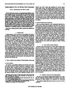
Figure 1: The block diagram of the proposed postprocessing algorithm, where W2rj f is the high-pass wavelet transform of f (x, y) in scale 2j of orientation r where j = 1, 2, 3 and r = 1, 2. S2r3 f denotes the low-pass wavelet transform of f (x, y) in scale 23 .
Figure 2: 1-D edge model.
2
Postprocessing Algorithm Using Multiscale Edge Characterization
Normally, images have two perceptual properties, sharp edges and smooth continuous regions. From [20], we know that the image reconstructed from its thresholded WMMR can retain these two visually important properties. However, these properties deteriorate as a result of low bit-rate wavelet coding. Sharp edges become blurred and containing ringing errors. Low varying regions contain graininess and blotches, and are no longer smooth. The similar distortions are also introduced in the OWE of the coded image. Therefore, the approaches to characterize these distortions and to restore wavelet modulus maxima are essential to effective image postprocessing. In this section, the study is divided into three parts. Firstly, the WMMR technique based on the OWE is briefly reviewed in the 1-D case and applies to the 2-D case. Then, edge degradation is characterized as the distortion of wavelet modulus maxima, i.e., the magnitude decays, and we study the restoration of wavelet modulus maxima for image postprocessing on a synthetic image and real images. The former experiment provides an insight into the proposed algorithm for wavelet modulus maximum restoration. The latter derives a set of empirical compensation functions for coded real images at certain bit-rates. Finally, the postprocessing algorithm is developed according to the results obtained.
2.1
Edge Model and Wavelet Modulus Maximum Representation
Edges in an image have the local 1-D structure feature in the sense that there are sharp intensity changes in the perpendicular direction together with little or no change in the parallel direction. In [21], an edge was modeled as the convolution of a step function and a Gaussian function of variance σ 2 as, x c s(x; b, c, σ) = b + (1 + erf ( √ )), 2 σ 2
(1)
where erf (·) ∈ [−1, 1] is the scaled error function, x is the perpendicular distance from the center of an edge, w the width of the edge, c the contrast across the edge and b the intensity at the edge base. Fig. 2 depicts the parameters. In an image with x − y coordinate system, (1) becomes, c x cos θ + y sin θ √ s2D (x, y; b, c, σ, θ) = b + (1 + erf ( ), 2 σ 2 3
(2)
where an edge passes through the origin with a gradient angle θ from x-axis. For ease of explanation, we will consider the 1-D case, and use the edge degradation model for wavelet coding in [17] as s1 (x) = s(x; σ1 , b, c) + q(x) with σ1 = λ · σ ,
(3)
where the quantization noise q(x), or q(x, y) in the 2-D case, may correspond to the ringing effect and λ > 1.0 (λ ≈ 1.3 in [17]) is the widening factor related to the blurring effect. (3) characterizes the edge degradation by two elements, the widening factor λ, and the quantization noise q(x, y). In [20], it was shown that the OWE is closely related to multiscale edge detection by checking the local maxima of wavelet transform modulus at different scales. Moreover, the evolution of modulus maxima across scales enables the numerical characterization of edges of different types by two mathematical factors: Lipschitz exponent α and smooth factor σ. Given a 1-D function f (x), its wavelet transform at scale 2j is denoted by W2j f (x). A function f (x) is uniformly Lipschitz α over (a, b) if and only if there exist a constant K > 0 such that for all x ∈ (a, b), |W2j f (x)| ≤ K(2j )α .
(4)
Consider a function f0 (x) which is equal to the convolution of a singularity f (x) and a Gaussian function of variance σ 2 , then (4) becomes p |W2j f0 (x)| ≤ K(2j )sα−1 , with s = 22j + σ 2 . (5) 0 0 The parameters in (5), namely α, σ, and K, describe the properties of the sharp variation over (a, b), and can be estimated from the decay of wavelet modulus maxima of the OWE at different scales. Consider another singularity f1 (x) which is equal to the convolution of f (x) and a Gaussian function of variance λ2 σ 2 where λ > 1. If we assume that modulus maxima take the upper bound of the inequalities in (4) and (5), then the relation between f0 (x) and f1 (x) in terms of wavelet modulus maxima is shown as, |W2j f0 (x)| Π2j (λ, σ, α) = = |W2j f1 (x)|
µ
22j + σ 2 22j + λ2 σ 2
¶ α−1 2
(6)
which is only related to scale 2j , λ, the Lipschitz exponent α, and the smooth factor σ. For example when λ0 = 1.3, Π2j (λ0 , σ, α) is illustrated in Fig. 3 where we assume that the singularities in practical signals have Lipschitz factor −1 ≤ α ≤ 1 and smooth factor σ ∈ [0, 2]. It was shown in [20] that (4) and (5) still hold for negative Lipschitz exponents. From Fig. 3, we see that λ > 1.0 in f1 (x) introduces the
1.4
1.3
1.2
1.1
1 2
1.5
The modulus maximum decay ratio.
1.5
The modulus maximum decay ratio.
The modulus maximum decay ratio.
1.5
1.4
1.3
1.2
1.1
1 2 1
1.5 0.5
1
Smooth factor σ.
0.5
1
−1
Lipschitz factor α.
1.2
1.1
1
1.5 0.5
1
0 0.5
−0.5 0
1.3
1 2 1
1.5
0 0.5
1.4
Smooth factor σ.
0 0.5
−0.5 0
−1
Lipschitz factor α.
Smooth factor σ.
−0.5 0
−1
Lipschitz factor α.
(a) (b) (c) Figure 3: The illustration of Π2j (λ0 = 1.3, σ, α) where the vertical axis shows decay ratios, and the other two show −1 ≤ α ≤ 1 and σ ∈ [0, 2]. (a) j = 1. (b) j = 2. (c) j = 3. decay of wavelet modulus maxima compared to f0 (x). It is shown that when λ ∈ (1, 2), the modulus maximum decay ratios in the two finest scales, i.e. j = 1, 2, are significant, in particular when σ → 0 4
and/or α → −1. On the other hand, the decay ratios in scale 23 and so the corresponding modulus maxima very little with Lipschitz exponent α and smooth factor σ. Another important issue related to wavelet modulus maxima in one signal is to understand how much the signal information is carried by its wavelet modulus maxima and whether we can reconstruct the original signal from its wavelet modulus maxima. The algorithm proposed in [20] enables us to reconstruct most signals or images from their appropriately thresholded wavelet modulus maxima with sufficient precision. Particularly, the OWE of an image f (x, y) has two components, W21j f and W22j f , of the horizontal and vertical orientations respectively. The 2-D OWE of f (x, y) is referred as Wf = {W21j f (x, y), W22j f (x, y)}j∈Z .
(7)
(7) can be represented by the modulus functions M2j f (x, y) and the phase functions A2j f (x, y) as Wf = {M2j f (x, y), A2j f (x, y)}j∈Z .
(8)
Image processing usually involves the manipulation of a large amount of data. The WMMR technique enables us to develop image processing based only on the wavelet modulus maxima which are significantly fewer than pixels, such as compression in [20, 22], interpolation in [23], enhancement in [24], denoising in [25]. These approaches usually consist of three steps. Firstly, the selection of modulus maxima is conducted, and only important or related modulus maxima are chosen for further processing. Then the specific operations are performed on these selected modulus maxima instead of on all image data. Finally, the desired image is reconstructed from these processed wavelet modulus maxima using the WMMR technique in [20]. Since wavelet modulus maxima are the key elements that suffer the distortion from low bit-rate image coding, we study wavelet modulus maximum restoration as follows.
2.2
Multiscale Edge Analysis of Wavelet-Based Image Coding
Here we study the quantization noise q(x, y) and widening factor λ in (3) based the multiscale analysis using OWE. q(x, y) mainly consists of high-frequency components, and it dies out in the multiscale decomposition of OWE. Thus the effect of q(x, y) at the coarsest scale is negligible, and at the two finest scales, W21 f and W22 f , we apply a mask smoothing operator centered at each modulus maximum to (1−δ c )
2j reduce the influence of q(x, y). A smoothing mask operator is depicted in Fig. 4(a), where δ2nj = 8 c c c with 0 < δ2j < 1.0 and j = 1, 2. In this work, δ21 = 0.6 and δ22 = 0.8, which were found to be appropriate for most images.
7
8
9 9
8
7
6
6
5
δ δ
n 2j
n 2j
δ2
δ
n 2j
δ
c 2j
j
δ2
n 2j
δ
4
3
3 2
2 1 1
n 2j
1 1
2
2 3
3 4
4
δ2
5
n
n
n
δ
5
4
j
5 6
6 7
j
(a)
7 8
9 9
8
(b)
Figure 4: (a) Smoothing operator. (b) The mapping illustration. Now we study λ. It was assumed in (3) that wavelet-based coding introduces a widening factor λ > 1.0 to the edge width σ, but has little effect on the Lipschitz exponent and the position of the edge. From (6) and Fig. 3, we know that the widening effect from λ > 1.0 results in the decrease of wavelet modulus maxima at different scales. Therefore, if we can obtain a good estimation of Π2j (λ, σ, α), we can 5
restore the distorted modulus maxima and reconstruct the coded image using the WMMR technique. Thus, the characterization of λ can be changed to the estimation of the decay function Π2j (·). We have observed that the truncation of the same high frequency DWT coefficients may have different smoothing effects on edges with different gradient angle θ, i.e., λ = λ(θ). Hence, we may characterize Π2j (λ, σ, α) using a function ∆2j (θ) which is only dependent on the scale and the gradient angle. In summary, we have made two major assumptions in this work for modulus maximum restoration: (i) the wavelet-based coding process can be formulated by the zero-phase low-pass filtering process accompanied with the quantization error, as shown in (3), where the locations and Lipschitz exponent of the edge are unchanged; and (ii) the low-pass filtering effect of λ results in the decay of the wavelet modulus maximum which is only dependent on the gradient angle. To obtain the robust estimation of ∆2j (θ), we represent the gradient angles θ ∈ [0, 2π] by some finite section numbers i = 1, ..., L and we use L = 9. Fig. 4(b) shows the mapping of an angle θ ∈ [0, 2π] into i = 1, ..., 9 and this operation is denoted by L. Given an original image h(x, y) and its coded versionf (x, y), let their wavelet modulus maxima at scales 21 , 22 and 23 be {(M2j h(xjn , ynj ), A2j h(xjn , ynj ))n∈Z }j=1,2,3 ,
(9)
{(M2j f (xjn , ynj ), A2j f (xjn , ynj ))n∈Z }j=1,2,3 ,
(10)
and respectively. Based on the first assumption, the locations of the modulus maxima of f (x, y) and h(x, y) are the same at three scales. Hence, given the OWE of a coded image, the distortion of a modulus maximum is represented as the decay ratio which is related to its gradient angle, i.e., the section number of the gradient angle, and defined as ∆2j (i) =
M2j h(xj , y j ) M2j f (xj , y j )
(11)
where i = L(A2j h(xj , y j )) is the section number representing the gradient angle in the way shown in Fig. 4(b). Based on the second assumption about the interpretation of the edge degradation under the OWE, we can develop a set of compensation functions from {∆2j (i)}j=1,2 to restore the wavelet modulus maxima of a coded image for postprocessing. In the following, we will conduct two experiments to investigate {∆2j (i)}j=1,2 , performed on a synthetic image and a set of real images, respectively.
(a) (b) (c) (d) Figure 5: (a) Original synthetic image h(x, y) (128×128, 8bpp). (b) Coded image f (x, y) (40.22dB)). (c) Initial reconstructed image g(x, y) (43.57dB). (d) Constrained reconstruction result g 0 (x, y) (43.60dB).
2.2.1
Experiments on a Synthetic Image
We first study a synthetic image h(x, y), shown in Fig. 5(a), which has identical edge model parameters along the circle curve, w = 1.0, c = 100 and b = 100 as defined in (1). We assume these values are 6
typical settings for edges in an original image. Note that h(x, y) has uniformly distributed gradient angles. The coded version of h(x, y), i.e., f (x, y), is shown in Fig. 5(b) which is obtained by zerotree quantization with the threshold Tq = 32. For most images coded at low bit-rates, Tq is 32. The 3-scale OWE of h(x, y) and f (x, y) are shown in Fig. 6(a)—(f). From M2j h(x, y) and M2j f (x, y), j = 1, 2, 3,
(a)
(b)
(c)
(d)
(e)
(f)
(g) (h) (i) Figure 6: The 3-scale OWE of the original image h(x, y), the coded one f (x, y), and the reconstructed one g(x, y). (a) M21 h(x, y). (b) M22 h(x, y). (c) M23 h(x, y). (d) M21 f (x, y). (e) M22 f (x, y). (f) M23 f (x, y). (g) M21 g(x, y). (h) M22 g(x, y). (i) M23 g(x, y). we compute the average decay ratios for wavelet modulus maxima with gradient angles in the same section and plot decay functions ∆2j (i) against the section number i = 1, ..., 9 for three scales 21 , 22 and 23 in Fig. 7(a), where we have two observations: (i) the distortions of modulus maxima are closely related to their gradient angles; and (ii) the finer is the scale, the greater are the distortions introduced, as seen in Fig. 3 . We explain the phenomena of Fig. 7(a) as follows. The degradation of edges in an image due to the zerotree quantization of DWT is mainly introduced by the quantization errors of small DWT coefficients in high frequency subbands. For edges of different gradient angles, the compaction of edge energy with respect to DWT primarily depends on the gradient angles. The closer is the gradient angle to the horizontal or vertical, the more edge energy can be compacted into fewer coefficients, thereby reducing the number of coefficients of small magnitude in high frequency subbands. Also, less low-pass filtering effect will be introduced by zerotree quantization. Therefore, the maximal distortion will happen to those edges of diagonal gradient angle (i.e. with the section number i = 5.) and the modulus maxima with such gradient angles may bear the largest decaying error, as shown in Fig. 7(a).
7
1.35
2
Scale 1 Scale 2 Scale 3
1.3
1.9
1.7
1.6
1.2 p(θ)
Modulus maximum decay ratio
1.8
1.25
1.5
1.15 1.4
1.1
1.3
1.2
1.05 1.1
1 1
2
3
4
5 6 Section number i
7
8
9
1
0
0.5
1 The normalized gradient angle θ.
1.5
(a) (b) Figure 7: (a) Decay functions, {∆2j (i)}j=1,2,3 . (b) The plot of p(θ) for θ ∈ [0, π2 ]. In this work, the modulus maximum restoration is only conducted on the two finest scales, 21 and 22 . Based on the above analysis and Fig. 7(a), we propose to recover the distorted modulus maxima of the coded image f (x, y) by a set of compensation functions {Λ2j (θ)}j=1,2 which is defined as Λ2j (θ) = ζj,1 p(θ) + ζj,2 with j = 1, 2 and 1 , p(θ) = max(cos2 (θ), sin2 (θ))
(12) (13)
where ζj,1 and ζj,2 are empirical factors, and p(θ) is the scaled compensation function, as shown in Fig. 7(b). For the coded image in Fig. 5(b) and from Fig. 7(a) we set ζ1,1 = 0.25, ζ1,2 = 0.90, ζ2,1 = 0.20, ζ2,2 = 0.85. These particular compensation functions were chosen for two reasons: (i) we assume that the modulus maximum distortion is proportional to the reciprocal of the maximum oriented edge energy projection, i.e., the horizontal one or the vertical one, represented by sin2 (θ) and cos2 (θ), respectively; and (ii) the modulus maximum distortion should be symmetric about i = 5. To evaluate the effectiveness of {Λ2j (θ)}j=1,2 , we apply them to the modulus maximum restoration of the OWE of the coded image f (x, y) as follows. M2j g(xjn , ynj ) = M2j f (xjn , ynj ) · Λ2j (A2j f (xjn , ynj )),
(14)
where M2j g is the reconstructed OWE of M2j f . The numerical results of the modulus maximum restoration are listed in Table I, and compared with those of the original image in terms of the standard deviation (stdev) and the mean. The result of the constant compensation, {M2j k(xjn , ynj )}n∈Z, j=1,2 , which can only restore the mean of modulus maxima, is also listed in Table I for comparison. It is shown that {Λ2j (θ)}j=1,2 produces good restoration results with both the stdev and the mean of the restored modulus maxima close to the originals. Then, using the reconstruction algorithm in [20] and the same wavelet transform at 23 scale, i.e., M23 f (high-pass) and S23 f (low-pass), an image can be reconstructed from wavelet modulus maxima of three groups {M2j f (xjn , ynj )}n∈Z, j=1,2 , {M2j g(xjn , ynj )}n∈Z, j=1,2 , and {M2j k(xjn , ynj )}n∈Z, j=1,2 , respectively. The PSNR of the reconstructed image is computed with respect to the original image as a function of the number of iterations, as shown in Fig. 8. We can see that the image reconstruction from {M2j g(xjn , ynj )}n∈Z, j=1,2 is the best one with the highest PSNR, as shown in Fig. 5(c). The reconstructed OWE {M2j g(x, y)}j=1,2,3 are also shown in Fig. 6(g), (h) and (i), where we see that most wavelet modulus maxima are appropriately stretched and the quantization noise q(x, y) is greatly suppressed. However, it is also observed that some large restoration errors may occur due to the inaccurate estimation of phases of wavelet modulus maxima. Thus the smoothing mask operator in Fig. 4(a) could be applied to all restored modulus maxima to reduce restoration errors. However, when Λ2j (θ) was applied to real images we could not obtain the same good restoration results. This is probably due to the fact that the synthetic image shown in Fig. 5 may not be a good representation 8
of an average image. Unlike the synthetic image, real images contain many edges of different model parameters, Lipschitz exponents, and other distinct properties. Although the simple characterization of the synthetic image provides a clear insight of the distortion of wavelet modulus maxima, it fails to derive an effective restoration method for real coded images. To achieve more accurate modulus maximum restoration for real images, we will conduct experiments on a set of real images. Table 1: Comparison of wavelet modulus maximum restoration. Modulus maxima of wavelet transform {M2j h(ujn , vnj )}n∈Z {M2j f (ujn , vnj )}n∈Z {M2j g(ujn , vnj )}n∈Z {M2j k(ujn , vnj )}n∈Z
j = 1 (Scale 21 ) mean stdev 72.50 3.65 60.80 5.76 71.51 4.09 72.50 6.83
j = 2 (Scale 22 ) mean stdev 105.53 4.13 96.51 7.82 106.34 6.61 105.53 8.53
44 43 42 Image Reconstructed from Mg(x,y) Image Reconstructed from Mk(x,y) Image Reconstructed from Mf(x,y)
41
PSNR
40 39 38 37 36 35 34 0
2
4
6
8 10 12 Number of Interations
14
16
18
20
Figure 8: PSNR of the reconstructed image with respect to the iteration number.
2.2.2
Experiments on Real Images
Now we shall study the distortion of wavelet modulus maxima on ten real images (512 × 512, 8bpp) and their coded versions (coded by SPIHT [11] at 0.1bpp), as shown in Fig. 9. The OWE is computed for both sets of images, and then, the average modulus maximum decay ratios at the two scales are plotted against the section number in Fig. 10(a), from which we can see that decay ratios of wavelet modulus maxima are also closely related to their gradient angles in a similar way to the synthetic image shown in Fig. 5(a). In the following, we apply the operation of α = N (θ) and N = arg | cos(θ)| to normalizing any gradient angle θ ∈ [0, 2π] into α ∈ [0, π2 ]. Two plots of the average decay ratios shown in Fig. 10(a) are not symmetric about i = 5. We believe, if more images are used to compute the average, then two plots should be symmetric about i = 5 or α = π4 . Therefore, the final compensation functions {Γ2j (α)}j=1,2 are constructed to be symmetric about α = π4 by using the average of {∆2j (i)}j=1,2 and {∆2j (10 − i)}j=1,2 . {Γ2j (α)}j=1,2 can be further characterized by using the polynomial fitting approach, e.g. the polyfit function in Matlab, and it can be a general approximation to the expected decay function of wavelet modulus maxima of real images coded at 0.1bpp, and will be used for postprocessing images coded at 0.1bpp.
9
Figure 9: The real 10 images used in this work to exploit the compensation functions. 1.6
Simulated modulus maximum decay ratio
1.6
Modulus maximum decay ratio
1.5
Decay ratios at the scale j=1 Decay ratios at the scale j=2
1.4
1.3
1.2
1.1
1
1.5
1.4
1.3
1.2
1.1
1 1
2
3 4 5 6 7 Section number of the gradient angle i
8
9
0
0.2
0.4
0.6 0.8 1 Normalized gradient angles
1.2
1.4
1.6
(a) (b) Figure 10: (a) Average decay functions {∆2j (i)}j=1,2 . (b) Compensation functions {Γ2j (α)}j=1,2 . 2.2.3
Analysis of the Two Experiments
Comparing Fig. 7(a) and Fig. 10(a), we have two facts: (i) decay ratios of wavelet modulus maxima at two scales, 21 and 22 , in Fig. 7(a) vary with the section number i much more than those of Fig. 10(a); and (ii) the modulus maximum decay ratios at two scales in Fig. 7(a) are smaller than those of Fig. 10(a). We explain these two facts as follows. In general, the precise characterization of modulus maximum distortion is too complicated to obtain. To capture the general tendency of the relationship between gradient angles and decay ratios, we have used the average operation in Section II-B.2 to weaken the fluctuation effect of other subordinate factors and focus on the main one, i.e., the gradient angle. Therefore, the variation in the averaged plot is also reduced due to this approximation operation. On the other hand, real images usually contain abundant irregular edges which have negative Lipschitz exponents α < 0, resulting larger decay ratios compared to edges of α > 0, as shown in (3). Moreover, the energy of edges of α < 0 is more dispersed in the DWT, leading to more low-pass filtering effect from the zerotree quantization. Therefore, decay ratios of the modulus maxima of real images are larger than those of the synthetic image. Nevertheless, both Fig. 7(a) and Fig. 10(a) show that our assumption about the relationship between decay ratios and gradient angles holds for both the synthetic image and real images. In other words, the modulus maxima of diagonal gradient angles undergo the largest decaying errors from the wavelet-based coding, and the decay functions are nearly symmetric about the diagonal direction. Next, we will apply this simplified characterization to image postprocessing.
2.3
Postprocessing Algorithm
In practice, it is difficult to obtain a precise characterization of the modulus maximum distortion, and our study is mainly based on the empirical analysis and experimental results of a synthetic image and a set of real images. The compensation functions, {Γ2j (α)}j=1,2 allow us to restore the wavelet modulus 10
maxima of images coded at certain bit-rate, i.e. 0.1bpp. Now, we propose the postprocessing algorithm as shown in Fig. 1. Specifically, the proposed algorithm consists of three steps which are: selection of modulus maxima, restoration of modulus maxima, and constrained image reconstruction. Since the OWE at the two finest scales {(M2j f (x, y)}j=1,2 bear major distortions, the algorithm processes modulus maxima at only the two finest scales. The criteria of selection of modulus maxima is similar to those used in [26, 23], i.e., the intensity values and the length of edge curves. We set the thresholds of modulus maxima T21 = 10 and T22 = 15, and the length thresholds of edge curves L21 = 5 and L22 = 10. These empirical settings are found appropriate for tested images in our simulation. Hence, only modulus maxima belonging to edge curves with sufficient lengths and of adequate magnitudes are selected. We expect that those selected modulus maxima will allow us to reconstruct the most important edge structures in a coded image. Secondly, for each selected wavelet modulus maxima, we need to restore them by {Γ2j (α)}j=1,2 . Here, we assume that the normalized gradient angle α undergoes no distortion. Thus, we restore the distorted modulus maximum M2j f (ujn , vnj ) as M2j k(ujn , vnj ) = M2j f (ujn , vnj ) · Γ2j (N (A2j f (ujn , vnj ))),
(15)
where n ∈ Z, {M2j k}j=1,2 is the initially reconstructed OWE of {M2j f }j=1,2 . Furthermore, in order to keep the consistency of the restored modulus maxima of {M2j k}j=1,2 along edge curves and reduce the restoration errors, the smoothing mask operator, as defined in Fig. 4(a), is applied to each restored modulus maximum. We use {M2j g}j=1,2 to denote the smoothed version of {M2j k}j=1,2 . Then we represent the restored and smoothed modulus maxima of {M2j g}j=1,2 by W21j g(ujn , vnj ) = M2j g(ujn , vnj ) · cos(A2j f (ujn , vnj ))
(16)
W22j g(ujn , vnj )
(17)
=
M2j g(ujn , vnj )
·
sin(A2j f (ujn , vnj )).
Thirdly, from (16) and (17), we can reconstruct a coded image by using the WMMR technique [20], where we can incorporate two a priori constraints into the reconstruction operation to impel the reconstructed image close to the original one. The two constraints are the sign constraint in [20] and the zerotree quantization constraint of the DWT in [17]. To reduce the computation complexity, we can apply the latter constraint only once after a stable reconstruction result g(x, y) is obtained by the iterative 0 reconstruction algorithm. Thus, g (x, y) is the final reconstructed image, as shown in Fig. 5(d). The WMMR technique using the iterative image reconstruction algorithm in [20] converges quickly, usually in 5 to 10 steps. It was also proved that the WMMR algorithm converges exponentially, with the convergence rate larger than a constant. In practice, the computational speed of the proposed approach is less than 1 minute for a typical 512 × 512 image on a Pentium 400 MHz computer.
3
Experimental Results
The new method is tested on four real images, excluding those in Fig 9. All images are coded by SPIHT [11] at 0.1bpp, and we apply {Γ2j (α)}j=1,2 shown in Fig. 10(b) to restore wavelet modulus maxima. The results show that both visual quality and image fidelity can be improved with reduced coding artifacts around edges and among continuous regions. The PSNR gains of four images are shown in Table II, and visual improvements of two images are given in Fig. 11, where we also compare the proposed method with the one in [17]. It is shown that both methods provide similar PSNR gains, and they can reduce coding artifacts around edges. Since the new approach reconstructs the whole image, it also reduces the coding artifact among smooth regions, and we can see that the continuous regions are smoother than those from [17]. However, the computational complexity is higher than that of the edge reconstruction in [17], which recovers only edges. Strictly speaking, the precise characterization of modulus maximum distortion depends on images, bit-rates, and types of edges, which is too hard to obtain. Moreover, the fact of the phase distortion 11
Table 2: PSNR(dB) of Reconstructed Images (512 × 512, coded at 0.1bpp). Algorithms This work [17]
Lena PSNR Gain 30.40 +0.18 30.45 +0.23
Peppers PSNR Gain 30.14 +0.30 30.10 +0.26
Flower PSNR Gain 32.27 +0.25 32.34 +0.32
Monarch PSNR Gain 27.14 +0.50 27.11 +0.47
also complicates the analysis. Here, we have simplified the problem by assuming that all images coded at the same low bit-rate, e.g. 0.1bpp, suffer the same modulus maximum distortion which is only dependent on the edge gradient angle. Since there is no constraint on the bit-rate of image coding, one may be concerned with the efficiency of the proposed method on medium or high bit-rates. Actually, the key operation of the proposed algorithm is the stretch of wavelet modulus maxima, which allows the reproduction of edge sharpness. Although the selection of modulus maxima may lose some low intensity edges, we can recover them by the zerotree quantization constraint of the DWT that only keeps the useful modifications to DWT coefficients. In practice, for medium or high bit-rates, the proposed postprocessing algorithm preserves detailed structures and keeps the PSNR almost unchanged. This is probably because the proposed method performs little on images coded at medium or high bit-rates.
4
Conclusions
In this paper, we have proposed a new postprocessing approach for low bit-rate wavelet-based image coding using the WMMR technique. Particularly, edge degradation is characterized as the decay of modulus maxima of the OWE, and a set of compensation functions have been derived for the modulus maximum restoration. We expect that better restoration results can be obtained by using some adaptive schemes together with compensation functions that are fine tuned to the types of edges.
References [1] Y. Yang, N. P. Galatsanos, and A. K. Katsaggelos, “Regularized reconstruction to reduce blocking artifacts to the block discrete cosine transform compressed images,” IEEE Trans. Circuit Syst. Video Technol., vol. 3, no. 6, pp. 421–432, Dec. 1993. [2] R. L. Stevenson, “Reduction of coding artifacts in transform image coding,” in Proc. Int. Conf. Acoust Speech Signal Proc., Minneapolis, MN, 1993, vol. V, pp. 401–404. [3] R. Rosenholtz and A. Zakhor, “Iterative procedure for reduction of blocking effects in transform image coding,” IEEE Trans. Circuit Syst. Video Technol., vol. 2, pp. 91–95, March 1992. [4] S. Minami and A. Zakhor, “An optimization approach for removing blocking effects in transform coding,” IEEE Trans. Circuit Syst. Video Technol., vol. 5, no. 2, pp. 74–84, April 1995. [5] Y. Yang and N. P. Galatsanos, “Removal of compression artifacts using projections onto convex sets and line process modeling,” IEEE Trans. Image Processing, vol. 6, no. 10, pp. 1345–1357, Oct. 1997. [6] T. P. O’Rourke and R. L. Stevenson, “Improved image decompression for reduced transform coding artifacts,” IEEE Trans. Circuit Syst. Video Technol., vol. 5, no. 6, pp. 490–499, Dec. 1995. [7] J. Luo, C. Chen, and K. J. Park, “On the application of gibbs random field in image processing: form segmentation to enhancement,” Journal of Electronic Imaging, vol. 4, no. 2, pp. 187–198, April 1995. [8] J. Luo, C. W. Chen, K. J. Parker, and T. S. Huang, “Artifact reduction in low bit rate DCT-based image compression,” IEEE Trans. Image Processing, vol. 5, no. 9, pp. 1363–1368, Sept. 1996. [9] Z. Fan and R. Eschbach, “JPEG decompression with reduced artifacts,” in Proc. of SPIE 1996 Symposium on Image and Video compression, Vol. 2186, Feb. 1996, pp. 50–55. [10] J. M. Shapiro, “Embedded image coding using zerotrees of wavelet coefficients,” IEEE Trans. Signal Processing, vol. 41, no. 12, pp. 3445–3663, 1993.
12
[11] A. Said and W. A. Pearlman, “A new fast and efficient image codec based on set partitioning in hierarchical trees,” IEEE Trans. on Circuits Syst. Video Technol., vol. 6, no. 3, pp. 243–250, June 1996. [12] Z. Xiong, K. Ramchandran, and M. T. Orchart, “Wavelet packet image coding using space-frequency quantization,” IEEE Trans. Image Processing, vol. 6, no. 5, pp. 677–693, May 1997. [13] J. Luo, C. Chen, and K. J. Paker, “Image enhancement for low bit rate wavelet-based image compression,” in Proc. of 1997 IEEE Int. Sym. Circuits and Systems, Hong Kong, June 1997, pp. 1081–1084. [14] J. Li and C.-C. J. Kuo, “Coding artifact removal with multiscale postprocessing,” in Proc. of 1997 IEEE Int. Conf. Image Processing, Santa Barbara, CA, 1997, vol. 2, pp. 529–532. [15] M.-Y. Shen and C.-C. J. Kuo, “Artifact reduction in low bit-rate wavelet coding with robust nonlinear filtering,” in Proc. of IEEE Second Workshop on Multimedia Signal Processing, 1998, pp. 480–485. [16] M.-Y. Shen and C.-C. J. Kuo, “Real-time compression artifact reduction via robust nonlinear,” in Proc. of 1999 IEEE Int. Conf. Image Processing, Kobe, Japan, 1999, vol. 2, pp. 565–569. [17] G. Fan and W. K. Cham, “Model-based edge reconstruction for low-bit-rate wavelet transform compressed images,” IEEE Trans. on Circuits Syst. Video Technol., vol. 10, no. 1, pp. 120–132, Feb. 2000. [18] Z. Xiong, M. T. Orchard, and Y.-Q. Zhang, “Deblocking algorithm for JPEG compressed images using overcomplete wavelet representations,” IEEE Trans. on Circuits Syst. Video Technol., vol. 7, no. 2, pp. 433–437, April 1997. [19] T.-C. Hsung, D. P.-K. Lun, and W.-C. Siu, “A deblocking technique for block-transform compressed image using wavelet transform modulus maxima,” IEEE Trans. Image Processing, vol. 7, no. 10, pp. 1488–1496, Oct. 1998. [20] S. Mallat and S. Zhong, “Characterization of signals from multiscale edges,” IEEE Trans. on PAMI, vol. 14, no. 7, pp. 710–732, 1992. [21] P. J. L. van Beek, Edge-Based Image Representation and Coding, Ph.D. thesis, Delft University of Technology, 1995. [22] J. Froment and S. Mallat, “Second generation compact image coding with wavelets,” Wavelets-A Tutorial in Theory and Applications (C. Chui, Ed.) New York: Academic, pp. 655–678, Jan. 1992. [23] S. G. Chang, “Image interpolation using wavelet-based edge enhancement and texture analysis,” M.S. thesis, University of California at Berkerly, 1995. [24] J. Lu, D. M. Hearly Jr., and J. B. Weaver, “Contrast enhancement of medical images using multiscale edge representation,” Optical Engineering, vol. 33, no. 7, pp. 2151–2161, July 1994. [25] S. Mallat and W. L. Huang, “Singularity detection and processing with wavelets,” IEEE Trans. Inform. Theory, vol. 38, no. 2, pp. 617–643, 1992. [26] K. Sauer, “Enhancement of low bit-rate coded image using edge detection and estimation,” Computer Vision, Graphics and Image Processing, vol. 53, no. 1, pp. 52–62, 1991.
13
(a)
(b)
(c)
(d)
(e)
(f)
Figure 11: Partial postprocessing results of two tested images. (a) Lena (coded by SPIHT at 0.1bpp, 30.22dB). (b) Reconstructed Lena ([17], +0.23dB). (c) Reconstructed Lena (this work, +0.18dB). (d) Monarch (coded by SPIHT at 0.1bpp, 26.63dB). (e) Reconstructed Monarch ([17], +0.47dB). (f) Reconstructed Monarch (this work, +0.50bpp).
14