The output gap: measurement, comparisons and assessment

The output gap: measurement, comparisons and assessment

Research Paper No. 44 June 2000

Iris Claus, Paul Conway, Alasdair Scott

Reserve Bank of New Zealand

RESERVE BANK OF NEW ZEALAND: Research Paper No. 44

1

© 2000 Reserve Bank of New Zealand First printing 2000

Published by the Reserve Bank of New Zealand, PO Box 2498, Wellington, NEW ZEALAND

The views here are those of the authors and do not necessarily reflect official positions of the Reserve Bank of New Zealand. All errors, omissions, and views expressed in this paper are the sole responsibility of the authors. This Research Paper may not be wholly or partially reproduced without the permission of the Reserve Bank of New Zealand. Contents may be used without restriction provided due acknowledgement is made of the source.

1.

Claus, Iris

2.

Conway, Paul

3.

Scott, Alasdair

ISSN 0110 523X

2


Acknowledgements We are especially grateful to the co-authors of some of the Discussion Papers on which this Research Paper is based: David Frame, Victor Gaiduch and Ben Hunt. In addition, we would like to acknowledge the support and insightful comments of Adrian Orr. The valuable assistance of Dean Minot is also appreciated. Finally, we would like to thank colleagues who have commented on earlier versions of this work: Anne-Marie Brook, Aaron Drew, Gaylene Hunter, John McDermott, Chris Plantier and Christie Smith.


3

4


Contents Figures and tables

6

Summary

7

Chapter 1 The output gap and its measurement

9

1.1 1.2 1.3 1.4

The concept of the output gap Measurement of the output gap Three output gap models used at the Reserve Bank Data and results

Chapter 2 Assessing the different output gap measures 2.1 2.2 2.3

Time domain analysis Frequency domain analysis Conclusion

Chapter 3 The use of the output gap under uncertainty 3.1 3.2 3.3 3.4

Measures of the output gap and inflation Output gap uncertainty and monetary policy rules Is the output gap still useful? Conclusion

References Appendix A1 Appendix A2 Appendix A3 Appendix A4

9 10 13 20 24 24 31 37 38 38 44 46 50 51

Estimation techniques Data and data sources The Fourier and wavelet transforms Integration tests


55 61 62 67

5

Figures and tables Figure 1 Figure 2 Figure 3 Figure 4 Figure 5 Figure 6 Figure 7 Figure 8 Figure 9 Figure 10 Figure 11 Figure 12 Figure 13 Figure 14 Figure 15

Artificial series with different trends Time series used in the estimation of the output gap measures Measures of potential output Measures of the output gap Peaks and troughs in the output gap measures Phase behaviour of the MV and UC output gap measures Phase behaviour of the MV and SVAR output gap measures Phase behaviour of the UC and SVAR output gap measures Estimated spectral densities of the output gap measures Wavelet decompositions Adjusted measures of the output gap Measures of the output gap and inflation Actual and predicted changes in inflation Actual and forecast changes in inflation The efficient frontiers

12 21 23 23 25 30 30 31 33 34 35 39 41 43 49

Figure A1 Figure A2 Figure A3

Periodic time series and spectral density Time series of three different frequencies and spectral density Wavelet coefficients

63 64 66

Table 1 Table 2 Table 3 Table 4 Table 5 Table 6 Table 7 Table 8 Table 9

Descriptive statistics Descriptive statistics (cont.) Correlation statistics Concordance statistics Spectral mass within business cycle frequencies Estimation results Variance decomposition of the change in inflation Out-of-sample forecasts of inflation changes Statistical properties of simulated output gap errors

26 27 28 29 33 40 42 44 47

Table A1 Table A2

Integration tests for the SVAR model Integration tests for the inflation models

58 67

6


Summary In recent years, many central banks have moved to pursue explicit inflation targets. Because of the long lags between policy actions and inflation outcomes, indicators of future inflationary pressures play an important role in guiding monetary policy aimed at achieving price stability. The output gap is considered to be a key indicator of future (domestic) inflation; hence it has an important role in a forward-looking inflation-targeting framework. The output gap is simply the difference between actual output and potential output. In turn, potential output is the level of economic activity that is consistent with no inflation pressures in the economy. In this sense, potential output is the level of activity that the economy can sustain, given its productive capacity. All else equal, if the output gap is positive through time, so that actual output is greater than potential output, then inflation will begin to increase in response to demand pressures in key markets. The converse will apply if the output gap is negative. Given its importance, the output gap has been the focus of considerable research effort at the Reserve Bank of New Zealand during the last few years. This research has been conducted on three fronts. First, various techniques for estimating potential output and the output gap have been developed. Second, the resultant estimates have been rigorously compared to assess their similarities and differences. The third research direction has investigated the policy implications of the significant uncertainty associated with these estimates of the output gap. This Research Paper presents the results of this ongoing work. The volume is organised into three chapters that cover these themes. The first chapter discusses the theoretical foundations of the output gap and various ways in which it has been measured. Potential output is determined by factors such as the level of technology, the abundance and quality of productive resources and the microeconomic environment. However, for a number of reasons, it has generally proved impracticable to estimate potential output on the basis of these fundamentals. At the Reserve Bank, three models have been developed that infer the level of potential output from observable macroeconomic data. These models decompose real output into a trend and a cyclical component. The trend is interpreted as a measure of the economy’s potential output (supply) and the cycle is interpreted as a measure of the output gap (demand). The first model, the multivariate filter, produces the measure of the output gap used in the Reserve Bank’s economic projections. The multivariate filter augments a common time-series filter with conditioning information from structural economic relationships. Specifically, information from inflation,


7

unemployment and surveyed capacity utilisation is used to help decompose actual output into measures of potential output and the output gap. The multivariate filter imposes some restrictions on the dynamics of potential output and the output gap. Two alternative estimation techniques used at the Reserve Bank are less restrictive in this respect. Both of these techniques estimate potential output and the output gap within a system of equations. The first alternative technique is based on a structural vector autoregression methodology. This technique uses a system consisting of output, employment and capacity utilisation to identify potential output and the output gap. The second technique employs a multivariate unobserved components approach. This technique decomposes observed output into three unobserved components: a permanent trend (potential output), a trend-reverting cyclical component (the output gap) and random noise. The cyclical component is assumed to be related to an underlying cycle in the economy, which is also present in unemployment and capacity utilisation. In chapter 2, the estimated output gaps from these models are compared using a variety of different techniques. This analysis suggests that the various output gap measures share some important similarities. In particular, all of the output gaps ‘co-move’ and, more often than not, are in agreement about the state of the cycle, especially during the 1970s and 1990s. During the 1980s, however, the output gaps are less similar, highlighting the difficulties of distinguishing supply and demand shocks during this period of economic reform in New Zealand. During the 1990s the output gap estimates appear to converge, which may imply the emergence of a more regular growth cycle in the New Zealand economy. Although the output gap measures tend to indicate consistently whether the economy is in excess demand or supply, there is often substantial disagreement about the severity of cycles. In other words, there is uncertainty about the magnitude of the output gap. This highlights the uncertainty that is an inherent feature of output gap estimates. The policy implications of this uncertainty are investigated in chapter 3. Despite uncertainties, the output gap estimates are found to be significant determinants of inflationary pressures. Furthermore, the various output gaps are reasonably proficient at forecasting near-term changes in inflation. This chapter goes on to consider the implications of output gap uncertainty on simple rules for conducting monetary policy. This analysis suggests that policymakers should temper the aggressiveness of their response to movements in the output gap in light of associated uncertainty. However, even in the presence of uncertainty, the output gap still has a valuable role to play in the policy process. Using the output gap to guide policy actions leads to greater macroeconomic stability than does basing policy actions solely on current, observable data. The output gap provides a link between the real economy and inflation and remains an important indicator of future inflationary pressures at the Reserve Bank of New Zealand. However, because a range of other factors also influence inflation, the output gap takes its place in a broad inflationtargeting framework. Hence, the output gap is always viewed in context with other indicators. If it is used in this way, and not accorded spurious accuracy, it has a valuable role to play.

8


1 The output gap and its measurement The first section of this chapter defines the output gap and provides a brief chronology of its development. Section 1.2 outlines the different approaches that have been used to measure potential output and the output gap. Three models of the output gap developed at the Reserve Bank of New Zealand are discussed in more detail in section 1.3. The results from these three models are presented in section 1.4.

1.1 The concept of the output gap It is straightforward to define the output gap as the difference between the level of actual output and potential output. Since we can readily observe actual output, this naturally leads us to focus on the definition of potential output. Potential output can be defined in terms of the factors of production. For instance, Artus (1977) defines it as the level of output “that would be realised if the labour force … were fully employed, and labour and capital were used at normal intensity”. However, this expression is not particularly succinct – ‘labour force’, ‘fully employed’, and ‘normal intensity’ are all subject to considerable variation in interpretation and measurement. This variation, at least in part, explains the lack of a single, unique definition of potential output. From a central banking perspective, potential output is typically defined as the level of output that is consistent with no inflation pressure in the economy. In this framework, the output gap is a summary indicator of the relative demand and supply components of economic activity. As such, the output gap provides a measure of the degree of inflation pressure in the economy and is an important link between the real side of the economy – the production of goods and services – and inflation. All else equal, if the output gap is positive through time, so that actual output is greater than potential output, then inflation will begin to move upwards in response to demand pressures in key markets.1 The idea that economic growth tends to fluctuate around a sustainable rate has a reasonably long history in the economics literature, dating back at least to Fisher (1933). Such an idea established a role for stabilisation policy, suggesting, for example, that demand management policies could be used to

1

This definition is consistent with Okun (1962), who defines potential output as being “the maximum production without inflationary pressure; or, more precisely … a point of balance between more output and greater stability”.


9

increase output when it is below its sustainable level. The link to the nominal side of the economy came with the short-run Phillips curve. In the original specification of the curve, the inverse of the unemployment rate was used as a proxy for excess demand for labour (Phillips 1958). Low unemployment spelled high excess demand and upward pressure on wages. The original version of the Phillips curve has undergone several modifications since 1958. It was transformed from a wage-change equation to a price-change equation, where prices are set by applying a constant mark-up to unit-labour cost. From the slope of the price-change Phillips curve, policymakers could then infer how much unemployment would be associated with any target rate of inflation. These early versions of the Phillips curve reflected the prevailing economic thinking in the 1960s that the supply side of the economy was deterministic, that is, it grew at a constant rate through time, and that changes in demand were the prime cause of economic fluctuations. In the early 1970s price expectations and a stochastic supply side were introduced into Phillips curve analysis. The demand variable was re-specified more explicitly in terms of excess demand. Originally defined as an inverse function of the unemployment rate, the demand variable was redefined as the gap between the ‘natural’ and actual rates of unemployment.2 The adoption of the unemployment gap in the Phillips curve finally recognised Samuelson and Solow’s (1960) finding that economic fluctuations can arise as the result of both demand and supply shocks. Accordingly, it became necessary to decompose unemployment into components attributable to changes in supply and demand in order to formulate appropriate policy responses. The inclusion of price expectations recognised the importance of expectations in the inflation process and was able to account for shifts in the Phillips curve. Okun’s (1962) law relates labour market conditions to conditions in the goods market, providing a link between the unemployment gap and the output gap. With the natural rate hypothesis of Phelps (1967) and Friedman (1968), this led to the notion that there is an equilibrium level of output consistent with stable long-run inflation (Modigliani and Papademos 1976). Clearly, a central problem with the concept of the output gap is that it cannot be directly measured. The level of potential output is unobservable and has to be inferred from available macroeconomic data. This is the issue to which we now turn.

1.2 Measurement of the output gap Three general approaches to measuring potential output and the output gap have been used to varying degrees. The first, and one that received early favour, was to estimate a production function based on factor inputs such as capital, labour, and possibly intermediate inputs such as energy. The second estimation approach uses times-series techniques to decompose actual output into potential output 2

10

The natural rate is the rate that prevails when expectations are fully realised and incorporated into all wages and prices.


and the output gap. This approach is currently the most common. Finally, survey data can be used to infer the extent of excess demand or supply in the economy by asking economic agents directly. These approaches are discussed in turn. If potential output is inherently a supply side concept then an intuitively obvious measurement approach is to estimate a production function – the relationship between an observed level of output and the amount of resources used in the production process. This relationship could then be used to calculate the level of output that would be produced if resources were ‘fully employed’ and used at ‘normal intensity’. The production function approach was common for industrial countries during the 1960s and 1970s. However, there are a number of difficulties in using this approach and its popularity has declined in recent years. First, it is not clear what the appropriate functional form for the production function should be. Second, in order to make estimation possible, productive inputs such as different types of labour, machinery, natural resources and intermediate inputs must be aggregated into a few variables, such as ‘capital’ and ‘labour’. This can often be problematic. For example, it is not clear how to aggregate stocks of capital at various stages of their life cycles into a single measure. Even if these technical issues can be resolved, it is not only the stock of capital and labour that matter for the level of potential output. The intensity at which these factors are utilised is also important. For example, relative price shocks, such as an oil price shock, can dramatically change the stock of capital that can be productively utilised. A third problem with the production function approach is that ‘technical progress’ must be explicitly modelled. However, technical progress is also unobservable and difficult to measure empirically. These issues are important in New Zealand. Adequate capital stock data are currently unavailable. Widespread macroeconomic reforms in the 1980s resulted in large-scale obsolescence of capital and dramatic adjustments in the life cycle profile of the aggregate capital stock. The issue of an effective labour force is also complicated in New Zealand, given changes in employment regulations and economic structure. Finally, the choice of functional form is non-trivial for a small open economy with a large agricultural sector. For these reasons, the production function approach has not received much attention in New Zealand (though see Gibbs 1995). The second, and most common, approach to estimating potential output and the output gap uses time-series techniques to decompose actual output into supply and demand components. Instead of the ‘bottom-up’ methodology of the production function approach, these techniques take a ‘top-down’ view of the output gap. Some of the earliest applications of time-series techniques simply assumed that potential output was a deterministic function of time that could be extracted using a linear regression (figure 1). This has the virtue of simplicity, but implies that the level of potential output grows deterministically through time. The corollary to this assumption is that all of the movements in real output about the time trend are interpreted as the result of demand shocks. This approach became


11

Figure 1 Artificial series with different trends value 30

value 30

25

25

20

20 Peak to peak trend

15

15

10

10

Stochastic trend (HP filter) Artificial series

5

5

Deterministic trend 0

0 0

15

30

45

60

75

90

time

increasingly inappropriate in the 1970s when (linear) trend growth rates in industrial countries declined and inflation accelerated. A related time-series technique, which does not imply a constant growth rate for potential output, is the ‘trend through peaks’ method (Klein and Summers 1966). This technique involves fitting linear trends between the cyclical peaks in the output series. The linear segment is then extrapolated until the next cyclical peak (figure 1). This approach is simple and avoids the assumption of a constant growth rate, but it has a number of unsatisfactory implications. For example, it defines potential output as the maximum attainable level of production in the short run, whereas policymakers have in mind a concept linked to a notion of long-run sustainability. Trends in economic time series are now typically modelled as stochastic processes (Nelson and Plosser 1982). This implies that movement in output can occur as a result of shocks to aggregate demand and shocks to potential output (supply). Figure 1 provides a stylised example of a stochastic trend. During the last 20 years or so a number of time-series techniques have been developed to extract a stochastic trend from real output data. These techniques use a broad range of statistical criteria and assumptions about economic structure to identify a trend. For example, simple linear filters such as the first difference filter and the well-known Hodrick and Prescott (1997) filter identify the trend in output based primarily on the statistical properties of the actual output series and have little economic content. Another notable technique that relies largely on statistical criteria is that of Baxter and King (1995). It uses a band pass filter to extract cycles from output in a particular frequency band. On the other hand, Cochrane (1994) estimates potential output based on assumptions about economic structure derived from the permanent income hypothesis. Blanchard and Quah (1989) develop a structural vector

12


autoregressive model that also estimates potential output and the output gap based on structural assumptions about the nature of economic disturbances. The third and final approach to estimating potential output and the output gap is based on responses to surveys. Since the output gap is a function of the economy’s productive capacity, an obvious measurement technique is to simply ask firms about their productive capacity. Survey responses used to construct measures such as ‘capacity utilisation’ indicate the state of cyclical activity, and this measure can be mapped to output to provide a measure of the output gap. Although this approach is intuitively appealing, it is also subject to a number of uncertainties. First, firms interpret survey questions differently and there is no guarantee that responses will be indicative of demand pressures. Also, output gap estimates based solely on surveys of capacity utilisation assume that the intensity with which labour is utilised remains constant, which may not be the case. Moreover, surveys usually have a limited response base. Often they are based largely on firms producing manufactured goods. This implies that the results may need to be qualified in a small open economy with large service and agricultural sectors. Because of these pitfalls, survey measures provide a potentially useful source of information on the state of the economic cycle, but typically should not be interpreted as a definitive measure of the output gap.

1.3 Three output gap models used at the Reserve Bank In this section we discuss three models used at the Reserve Bank to estimate potential output and the output gap. All of these models are examples of the time-series approach discussed in section 1.2. Furthermore, all three models use information from actual output and a number of other key macroeconomic time series, including a survey measure of capacity utilisation. From an econometric point of view, information contained in other time series may help identify the demand component of output. From an economic point of view, it is sensible to use information from different sectors of the economy to estimate potential output and the output gap. In this context, the output gap reflects an underlying cycle in the economy, present in a range of macroeconomic time series. The first model considered is the multivariate filter. This model produces the output gap measure used in the Reserve Bank’s economic projections. A detailed treatment of the multivariate filter can be found in Conway and Hunt (1997). The second model is an adaptation of the Blanchard and Quah (1989) structural vector autoregressive methodology. Claus (2000a) discusses this model in detail. The third model is an unobserved components model, presented in detail in Scott (2000a).


13

The multivariate filter The multivariate (MV) filter is ‘semi-structural’, in that it incorporates information from macroeconomic relationships into a well-known time-series filter, the Hodrick and Prescott (HP) filter.3 The HP filter calculates a trend output series that minimises the expression

Λ=

T

T −1

t =1

t =2

∑ ( yt − ytτ )2 +λ ∑ [( ytτ+1 − ytτ ) − ( ytτ − ytτ−1 )]2

(1)

where yt is the log of actual output and ytτ is its trend. The first term is the sum of squared deviations of trend output from actual output. The second term penalises variations in the growth rate of trend output. The parameter λ is a smoothness constraint that determines the degree to which those variations are penalised. The smaller the value of λ , the smaller the penalty on changes to trend output and the more closely trend output follows the actual output series. Conversely, the larger the value of λ , the larger the penalty on changes to trend and the smoother the estimate of the trend. For quarterly output data λ is usually set equal to 1600. Hodrick and Prescott chose this value on the basis of their prior views about the magnitudes of cyclical volatility and trend growth rates in US macroeconomic aggregates. In the context of estimating potential output, the value of λ reflects, at least implicitly, the relative importance of supply and demand shocks in the evolution of actual output. The larger the value of λ , the smoother the estimate of potential output (aggregate supply) and the larger the proportion of output variability ascribed to the output gap (aggregate demand). The extensive use of the HP filter in decomposing time series into trend and cyclical components has motivated research examining the accuracy of such decompositions. Harvey and Jaeger (1993), for example, show that setting λ = 1600 is suitable for US real gross national product (GNP), but may not be suitable for other output series. Cogley and Nason (1995) observe that the HP filter, when applied to persistent time series, can generate business cycle dynamics even when they are not present in the original data. Monte Carlo evidence presented in Guay and St-Amant (1996) implies that under plausible assumptions about the evolution of actual output, the HP filter may not accurately decompose output into its trend and cyclical component. These considerations suggest that the HP filter estimate of trend output may not be an ideal estimate of potential output. Another problem associated with using the HP filter to measure an economy’s level of potential output is the instability of estimates near the end of the sample period. Because the persistence of recent shocks to output is unclear, the HP filter cannot distinguish accurately permanent and temporary shocks at the end of the sample period. This can result in substantial revision to end-of-sample measures of potential output. This ‘end-point problem’ is common to all filtering techniques that use ‘future’ data

3

14

Other time-series methods of estimating potential output that mix aspects of structural and statistical techniques can be found in Laxton and Tetlow (1992), de Brouwer (1998) and Haltmaier (1996).


in estimating the current level of potential output. Because current estimates of potential output and the output gap generally underpin forecasts of near-term inflation, the end-point problem can be particularly serious for policymakers. Various strategies have been developed to improve the ability of the HP filter to identify potential output and the output gap. One approach is simply to alter the parameter λ in line with prior beliefs about the ratio of demand to supply shocks (Razzak and Dennis 1995). Another approach is to augment the estimate of trend output with a number of ‘conditioning’ constraints based on macroeconomic relationships. On the basis of Monte Carlo experiments, Laxton and Tetlow (1992) find that conditioning information from a Phillips curve relationship and an Okun’s law relationship improves the accuracy of HP-filter-based estimates of potential output. Finally, Butler (1996) conditions filter estimates of potential output at the end of the sample period using a long-run growth rate restriction on potential output to help overcome the end-point problem. Two of these strategies were incorporated into the MV filter. Specifically, the HP filter is augmented with conditioning information from a Phillips curve relationship, an Okun’s law relationship and survey data on capacity utilisation to help identify supply and demand disturbances in real output. A long-run growth rate restriction is also applied at the end of the sample period to alleviate the end-point problem. Changing the value of λ to reflect prior views on the relative incidence of supply and demand shocks was found to exert a minimal influence on the estimate of potential output. Therefore, the value of λ is set at 1600 over the entire sample period. There are cogent reasons for incorporating each of the conditioning relationships into the estimation process. Because supply and demand shocks have inherently different implications for inflation, a Phillips curve relationship should contain information relevant to the estimation of potential output. Accordingly, the Phillips curve depicted in equation (2) provides information that conditions the MV filter’s estimate of potential output4

π t = π te + A( L)( yt − ytτ ) + ε π , t

(2)

The variables π t and π te represent inflation and inflation expectations respectively. A( L ) is a polynomial in the lag operator and

ε π ,t is the residual.5 Inflation expectations are measured as a weighted

average of a survey measure of expected future inflation and the recent history of actual inflation outcomes. The natural rate hypothesis is also imposed. In the context of equation (2), this means that the coefficient on expected inflation is constrained to equal 1.6 4

Haltmaier (1996) and Gibbs (1995) also use information from the inflation process to condition estimates of potential output within an HP filtering framework. In Kuttner (1994), an unobservable components approach is used to estimate simultaneously potential output and the inflation process.

5

The lag operator is a linear operator that simply lags the following variable.

6

Note that this is a closed-economy Phillips curve. Initially, first and second differences of the nominal exchange rate (contemporaneous and lagged) were also included as explanatory variables in the Phillips curve. However, since this specification of the Phillips curve did not substantially change the estimate of potential output, exchange rate effects were removed from equation (2).


15

Okun’s (1962) law postulates a link between conditions in the labour market and conditions in the goods market and is considered to be one of the most robust empirical regularities in macroeconomics. All else equal, a movement of actual unemployment below its trend rate indicates a positive shock to aggregate demand. By incorporating an Okun’s law relationship, the MV filter recognises that labour market conditions may contain valuable information about disequilibrium in the goods market. Equation (3) illustrates the Okun’s law relationship used in the MV filter to condition the estimate of potential output

ut − 4 − utτ− 4 = b( yt − ytτ ) + ε u, t

(3) τ

where ut is the unemployment rate, ut is its trend, and

ε u, t is the residual. Deviations of actual

unemployment from trend are assumed to influence conditions in the goods market after a lag of 4 quarters. The coefficient, b , is imposed at 0.333, implying an Okun’s law coefficient of 3. This is consistent with the value of b obtained by estimating equation (3) in conjunction with the other components of the MV filter over the 1990s. It is also close to the estimate obtained for New Zealand by Gibbs (1995) of 0.35 and Okun’s (1962) original estimate of 0.35 to 0.40. The multivariate filter also uses information from the level of capacity utilisation in the economy to condition the estimate of potential output. Using the same economic intuition that underpins the Okun’s law relationship, a movement of capacity utilisation above its long-run or sustainable rate is interpreted as indicative of a positive shock to aggregate demand. Equation (4) depicts the relationship between the level of capacity utilisation relative to trend and the gap between actual and potential output

caput − caputτ = c( yt − ytτ ) + ε capu, t

(4)

τ Capacity utilisation is denoted caput , its trend is caput , and the residual is ε capu, t . The parameter c

is set equal to 1, implying that deviations of capacity utilisation from trend map directly into output gap space. This restriction is not rejected by the data when equation (4) is estimated in conjunction with the other components of the MV filter. Finally, the multivariate filter conditions on a long-run growth rate assumption of 3 percent over the last 12 quarters of history. This constraint helps offset the tendency of two-sided filters to allocate movements at the end of the sample period to the trend component (the end-point problem). The multivariate filter does not treat equations (2) to (4) as structural in a strict sense. Instead, the information contained in the above macroeconomic relationships is used in a relatively flexible fashion to aid in the identification of supply and demand shocks over the course of New Zealand’s recent economic history. Technical details on how the conditioning information is incorporated into the MV filter are given in appendix A1. Assumptions about the trend rate of unemployment and capacity utilisation are discussed in section 1.4.

16


A structural vector autoregression model The second technique used to estimate potential output at the Reserve Bank is a structural vector autoregression (SVAR) model based on the work of Blanchard and Quah (1989) and King, Plosser, Stock and Watson (1991). In comparison to the MV filter, the SVAR model imposes fewer assumptions about economic structure on the relationships between the variables in the system. Accordingly, SVAR models are often considered to be ‘data driven’ and designed to ‘let the data speak’. The SVAR model uses information from the labour market (full-time employment) and capacity utilisation to aid in the decomposition of actual output into a permanent trend component (supply) and a temporary cyclical component (demand). The trend is interpreted as a measure of the economy’s potential output and the cycle is interpreted as a measure of the output gap. In the first stage of the estimation process the interrelationships in the data are captured by regressing each of the three variables in the system on their own lags and the lags of the other variables, as in equations (5) to (7)

∆yt = α1 + Φ11 ( L)∆yt −1 + Φ12 ( L)ltgap −1 + Φ13 ( L )caput −1 + ε ∆y , t

(5)

gap l tgap = α 2 + Φ 21 ( L)∆yt −1 + Φ 22 ( L)lt −1 + Φ 23 ( L)caput −1 + ε l , t

(6)

caput = α 3 + Φ 31 ( L)∆yt −1 + Φ 32 ( L)ltgap −1 + Φ 33 ( L )caput −1 + ε capu , t

(7)

This system of equations is the ‘reduced form’ of the SVAR model. The variable ∆yt is the first difference of (log) real output, l tgap is the (log) deviation of employment from trend and caput is, as before, the level of capacity utilisation.7 The Φ ij ( L ) terms are polynomials in the lag operator and the α i ’s are constants.8 The variables

ε ∆y, t , ε l , t and ε capu, t capture unexplained shocks to the dependant variables

of the reduced form. The reduced form shocks are composites of the supply and demand shocks that drive potential output and the output gap respectively. To recover these structural shocks a minimal set of identifying restrictions is imposed on the system. The key identifying restrictions are that, in accordance with the natural rate hypothesis, demand shocks do not affect output in the long run whereas supply shocks do. It is this dichotomy between temporary (demand) and permanent (supply) effects on the variables of the system that allows for the complete identification of the structural shocks from the reduced form error terms.9 The restrictions are imposed on the long-run dynamics of the variables. The short-run dynamics are left unrestricted. 7

Output is first differenced so as to render it stationary. Employment is found to be trend stationary and expressed as deviation from trend. The SVAR estimate of potential output is reasonably robust to the specification of trend employment. Deviations of employment from a time trend were chosen to avoid the end-point problem of two-sided filters, such as a centred moving average. The results of unit root tests on all of the variables are in appendix A1.

8

Lag length tests that ‘tested down’ (using likelihood ratio tests) to the first significant lag in the reduced form favoured a lag length of 4. The initial number of lags in the lag length test was set equal to 8.

9

In addition, a number of technical restrictions are also imposed. These are documented in appendix A1.


17

Once the structural shocks have been recovered, the variables of the system can be expressed as the sum of current and past realisations of these shocks. For example, output growth in the current quarter can be expressed as the result of all the past and current shocks to supply and demand. This ‘moving average’ representation of the variables in the SVAR is depicted in equations (8) to (10)

∆yt = S11 ( L)υ tS + S12 ( L )υ tD1 + S13 ( L )υ tD2

(8)

ltgap = S21 ( L)υtS + S22 ( L)υtD1 + S23 ( L)υtD 2

(9)

caput = S31 ( L)υtS + S32 ( L)υtD1 + S33 ( L)υtD 2

(10)

where the Sij ( L) ’s are polynomials in the lag operator. The variable or, equivalently, a shock to potential output. The variables υt and D1

υtS is the permanent supply shock

υtD2 are temporary demand shocks

that are assumed to drive changes in the output gap. From equation (8) it is straightforward to decompose output growth into components attributable to potential output and the output gap. Growth in potential output at time t is calculated by simply cumulating the permanent supply shocks to output growth, as in equation (11)

∆ytτ = S11 ( L)υtS

(11) c

The component of output growth due to changes in the output gap, yt , is given by

∆ytc = S12 ( L)υtD1 + S13 ( L)υtD 2

(12)

Technical details about the identification of the SVAR model can be found in appendix A1.

A multivariate unobserved components model A multivariate unobserved components (UC) approach to the measurement of the output gap posits that observed output can be decomposed into an unobserved trend (potential output), a trend-reverting or cyclical component (the output gap) and random noise. Models following this approach include Kuttner (1994) and Apel and Janson (1999). The model presented here builds on the model by Clark (1989). One advantage of the UC approach is that output, which is a non-stationary series, can be modelled without any need for transformations such as differencing. Another advantage is that the trend and cyclical components of output are estimated simultaneously. Univariate unobserved components models of output, such as those in Watson (1986) and Harvey and Jaeger (1993), also have these features. However, when applied to New Zealand data, these univariate models are typically unstable and experience severe convergence problems, indicating that a strong distinction between a permanent trend component and a transitory cyclical component cannot be made on the basis of output data

18


alone. These problems provide additional motivation for a multivariate treatment of the problem. In addition to output, the UC model also uses data on unemployment and capacity utilisation. To implement the UC approach, three things are required from the model. First, an estimate of the unobserved cyclical component that is common to all three time series in the model is required. Second, the model must provide estimates of the unobserved permanent trends of output, unemployment, and capacity utilisation. Finally, estimates of the coefficients that describe the linkages from the cycle in output to unemployment and capacity utilisation are needed. To fill these requirements, observed output is decomposed into three unobserved components

( )

( )

yt = ytτ + zt + ε y ,t , E ε y , t = 0 , Var ε y, t = σ ε2y

(13)

τ where, as before, yt and yt are output and its permanent trend component (potential output) respec-

tively. The temporary cyclical component (the output gap) is represented by zt , and ε y, t is an irregular noise component. Observed unemployment is also decomposed into permanent, temporary and irregular components

ut = utτ + D( L) zt + ε u, t , E(ε u, t ) = 0 , Var(ε u, t ) = σ ε2u

(14)

τ Here ut represents unemployment and ut is its permanent trend component. The polynomial in the

lag operator, D( L ) , allows for an Okun’s law relationship that relates the cycle in unemployment to the common cycle, zt . The irregular component is denoted ε u, t . Capacity utilisation is decomposed in an analogous way

(

)

(

)

2 caput = caputτ + G( L ) zt + ε capu,t , E ε capu, t = 0 , Var ε capu,t = σ εcapu

(15)

with obvious notation. Hence, in this model, the cycle

zt is common to the equations for all three observed variables. The

underlying trends for output, unemployment and capacity utilisation are independent. The dynamics of the cyclical component are modelled as an autoregressive process. The underlying trends are all modelled as local linear trends. The model can be written in state-space form and estimated via the Kalman filter and exact maximum likelihood. Technical details and the parameter estimates can be found in appendix A1.


19

1.4 Data and results All the time series used in the estimation of the output gaps are graphed in figures 2a to 2e. The models are estimated using data from 1970q1 to 1999q3.10 The data used in the estimation is described in appendix A2. It is important to note that this data span encompasses a number of distinct episodes in New Zealand’s economic history. In very general terms, the 1970s were a turbulent period for New Zealand with a number of significant shocks, including the oil shocks and large swings in the prices of other commodities, impacting on the economy. The 1980s are generally regarded as the ‘reform decade’, during which the governments of the time embarked on a comprehensive programme of economic reform. This transformed the New Zealand economy from one of the most interventionist in the OECD to one of the most open and market-based. Finally, since the early 1990s, the New Zealand economy has experienced increased rates of economic growth relative to the 1970s and 1980s. At least partly as a result of these changes, the gross domestic product (GDP) series displays a number of pronounced low-frequency swings over the sample period. From the graph of output in figure 2a, it is not clear that there is any simple trend: the growth rate has varied considerably over the years. Nor is there much evidence of a cycle of regular periodicity. Disentangling the relative incidence of demand and supply shocks in this environment is a challenging task. All three estimation techniques use surveyed capacity utilisation to inform their respective estimates of potential output. From the graph in figure 2b, this series shows some clearly cyclical behaviour, with the periodicity of the cycle becoming longer over the course of the sample period. This suggests that capacity utilisation may provide useful conditioning information in the estimation of potential output and the output gap. The level of trend capacity utilisation imposed by the MV filter is set at 88 percent from the beginning of the sample period until 1991q2 – its mean level over that sample. It is increased by 1 percent over a four-quarter period thereafter. This upward shift in trend is made to reflect additional flexibility in the input of labour to the production process that may have resulted from the Employment Contracts Act (1991). The UC model’s estimate of trend capacity utilisation displays a lowfrequency cycle before rising slowly over the late 1980s and early 1990.11 This increase in trend provides some empirical justification for the increase in trend capacity utilisation imposed by the MV filter. The MV and UC techniques also use the level of unemployment to condition their estimates of potential output (figure 2c). The unemployment series appears to display cyclical dynamics, suggesting that this series will also help condition estimates of potential output and the output gap. The trend rate of unemployment used by the MV filter is estimated using a standard HP filter. The value of the smooth10

Note that the survey measure of expected inflation that is used by the MV filter begins in the first quarter of 1983. Given this constraint, the Phillips curve component of the MV filter is estimated over the period 1983q1 to 1999q3. The estimated coefficients are then imposed on the MV filter estimate of potential output over all of the sample period, ie 1970q1 to 1999q3.

11

Note that the UC trends of capacity utilisation and unemployment are the final estimates from the Kalman smoother, which revises the estimates from the Kalman filter for all information over the sample, rather than only up to time t .

20


ness parameter, λ , is set equal to 1600 in all periods except 1991q2, in which it equals zero. This allows for a break in the trend rate of unemployment, coinciding with the introduction of the Employment Contracts Act (1991).12 The UC estimate of trend unemployment is noticeably persistent and increases in large steps through the sample period. The MV filter also uses the rate of inflation, within the context of a Phillips curve, to condition estimates

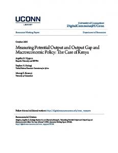
Figure 2 Ti m e s e r i e s u s e d i n t h e e s t i m a t i o n o f t h e o u t p u t g a p m e a s u r e s a) Output

b) Capacity utilisation % 4

log 10.1

3

10.0

2

9.9

1

9.8

0

9.7

-1 -2

9.6

-3

9.5

% 94

% 94

92

92

90

90

88

88

86

86

84

84

-4

9.4 1970

-5 1974

1978

1982

GDP

1986

1990

1994

1998

1978

1982

1986

1990

MV trend

1994

1998

UC trend

d) Inflation

% 12

% 12

10

10

8

8

6

6

4

4

2

2

0 1970

0 1978

82 1974

Capacity utilization

Change in GDP (rhs)

c) Unemployment

1974

82 1970

1982

Unemployment

1986

1990

MV trend

1994

1998

UC trend

% 18

% 18

16

16

14

14

12

12

10

10

8

8

6

6

4

4

2

2

0 1970

0 1974

1978 Inflation

1982

1986

1990

1994

1998

Surveyed inflation expectations

e) Employment log 7.25

log 7.25

7.20

7.20

7.15

7.15

7.10

7.10

7.05

7.05

7.00

7.00

6.95

6.95

6.90 1970

6.90 1974

1978

1982

Employment

12

1986

1990

1994

1998

SVAR trend

In practice the unemployment series is extended beyond its last historical observation using forecast data. The HP filter is then applied to the extended series to alleviate the end-point problem.


21

of potential output (figure 2d). Inflation was high and volatile during the 1970s and 1980s, before falling in the late 1980s and early 1990s. Finally, the level of employment and its trend, used in the SVAR model, are graphed in figure 2e. The MV, SVAR and UC estimates of potential output and actual output are graphed in figure 3. The associated output gap estimates are graphed in figure 4. For purposes of comparison, the HP filter estimate of the output gap, with λ = 1600, is also displayed. Although the various output gap estimates typically indicate a different level of the output gap at each point in time, there are periods of broad agreement. During the mid-1970s, all of the output gap measures indicate a period of excess demand, consistent with increasing inflationary pressures at this time. During the 1980s, there appears to be more disagreement about the relative incidence of supply and demand shocks, with the SVAR model and, to a lesser extent, the UC model indicating more excess demand than the MV and HP output gap estimates. The lack of consensus over this period may reflect the relative turmoil of economic reform and the associated structural adjustment. In this environment, it would almost be surprising if the different estimation techniques reached a similar view about the relative importance of supply and demand forces in the economy. During the early 1990s, the various output gap estimates once again tell broadly consistent stories. They indicate significant excess supply as the rigours of structural and fiscal adjustment, along with disinflation and a collapse in the New Zealand sharemarket, culminated in a very poor rate of economic growth. The degree of conformity in the output gap measures appears to increase throughout the 1990s. During the mid-1990s, the New Zealand economy grew strongly. All four measures of the output gap indicate that this led to a situation of excess demand (a positive output gap). In the late 1990s two consecutive droughts, the negative impact on foreign demand from the Asian financial crisis and the influence of recent tight monetary conditions (in response to strong inflation pressures) contributed to a short period of excess supply in 1998 and 1999. According to all four output gap estimates, actual output is approximately equal to potential output by the end of the sample period. In general terms, the SVAR and UC output gap estimates appear to display deeper and longer cycles relative to the MV and HP measures. For example, according to the SVAR and UC output gap estimates, the trough in the early 1990s cost 7 to 8 percent of potential output, and actual output was below potential for some 51/2 years. In comparison, according to the MV estimate of the output gap, this trough amounted to 4 percent of potential output and actual output was below potential for only 4 years. Finally, the output gaps estimated using the MV and HP filters appear to display similar cyclical characteristics. However, the level of the MV output gap estimate is often different to that of the HP output gap estimate.

22


Figure 3 Measures of potential output log

log

10.1

10.1

10.0

10.0

9.9

9.9

9.8

9.8

9.7

9.7

9.6

9.6

9.5

9.5

9.4 1971

9.4 1975

1979

1983 GDP

MV

1987 SVAR

1991

1995

1999

UC

Figure 4 Measures of the output gap %

%

8

8

6

6

4

4

2

2

0

0

-2

-2

-4

-4

-6

-6

-8 1971

-8 1975

1979

1983 HP


1987 MV

SVAR

1991

1995

1999

UC

23

2 Assessing the different output gap measures Given the range of output gap estimates, it is useful to illustrate their respective properties. The analysis presented in this chapter uses a number of analytical techniques to conduct a rigorous and detailed comparison of the output gap measures presented in chapter 1. These techniques fall into two categories. In section 2.1 we use time domain techniques to compare the output gap measures. As the name suggests, these techniques allow us to compare how the various measures of the output gap evolve through time. This allows us to assess, for example, the degree to which the output gaps co-move and share common turning points. This section is based on the work of Scott (2000b). In section 2.2 we compare the output gap estimates using frequency domain techniques. These allow us to assess how important cycles of different frequencies are in explaining each of the output gap estimates and thereby highlight important differences in their cyclical properties that may not be apparent in the time domain. The material in this section is from Conway and Frame (2000).

2 . 1 Ti m e d o m a i n a n a l y s i s This section presents a number of statistics that illustrate different properties of the cycles in the various measures of the output gap for New Zealand. For the purpose of comparison, the HP filter, with λ = 1600, measure of the output gap is included in the analysis. The output gaps are assessed with respect to differences in the average length and magnitude of cycles, whether cycles exhibit a regular periodicity and shape, whether they are symmetric in phase and severity of swings, and whether they share the same turning points. To do these comparisons, a method that dates the peaks and troughs of the output gap estimates is needed. To this end, a simple algorithm is applied which dates a peak as the highest point in the period during which output is above its trend (ie the output gap is positive). The opposite applies to date troughs. This is a very naïve dating rule, and it could be convincingly argued that the policymaker would never follow such a rule in practice. For example, this rule will pick a cyclical peak no matter how close that peak is to zero. In practice, however, because of the uncertainty surrounding the estimate of potential output and the output gap, a policymaker may want to distinguish between peaks that are ‘close enough’ to neutral and those that are ‘clearly’ in excess demand or excess supply.

24


However, mimicking a more realistic decision rule is non-trivial. Two alternative rules were experimented with. In the first, a three-quarter, one-sided moving average filter was applied to the gap estimates, simulating the actions of a policymaker attempting to filter out high frequency spurious noise from their decision making problem. This did not substantially change the results reported below. A second rule eliminated peaks and troughs within a certain distance of zero. However, aside from the subjectivity of the threshold choice, further ad hoc filtering was required to ensure peaks and troughs alternate. Experience with the gap estimates revealed that it was difficult to know when to stop filtering. The results would then be susceptible to the critique that the stylised facts were influenced by the dating rule. For these reasons it was decided to proceed with the simple dating rule. Figure 5 presents the HP, MV, SVAR and UC output gap estimates with peaks and troughs dated according to the naïve dating rule. As can be seen, the peak and trough dates suggested by the various output gap measures differ. The output gaps from the HP and MV filters are reasonably close in terms of cycle turning points, with both suggesting the existence of 7 cycles (trough-peak-trough) over the sample period. The simple dating rule identifies 5 cycles in the SVAR and UC output gap measures.

Figure 5 Peaks and troughs in the output gap measures a) HP

b) MV

c) SVAR

d) UC


25

However, the turning points are significantly different from each other and from the turning points of the HP and MV output gap measures.

The average duration and magnitude of contractions and expansions Average duration, magnitude, and magnitude per quarter for contraction and expansion phases are presented in table 1. ‘Duration’ is the length of time from trough to peak for an expansion phase and from peak to trough for a contraction phase. The ‘magnitude’ of an expansion (contraction) phase is the distance from the trough (peak) to the peak (trough). ‘Magnitude per quarter’ is the average magnitude of the contraction or expansion divided by its average duration. The average durations of cycles in the various measures of the output gaps are clustered in a range of 7 to 12 quarters for contractions and 8 to 12 quarters for expansions. For contractions and expansions, the SVAR and UC models produce an output gap with cycles of a longer duration than the HP and MV filters. The SVAR and UC output gap measures also have cycles of a larger magnitude than those of the HP and MV estimates.

Ta b l e 1 Descriptive statistics Contraction (peak to trough) Duration (quarters) HP MV SVAR UC Average

7.00 7.86 9.00 11.80 8.92

Expansion (trough to peak)

Magnitude (percentage points)

Magnitude/ quarter

Duration (quarters)

Magnitude (percentage points)

Magnitude/ quarter

-4.67 -4.49 -5.32 -5.50 -5.00

-1.13 -0.77 -0.64 -0.53 -0.77

8.00 7.57 12.00 9.60 9.29

4.84 4.31 5.47 5.75 5.09

0.85 0.85 0.47 0.58 0.69

The symmetry and severity of contractions and expansions All of the output gap estimates are approximately symmetric. For each measure, the average duration, magnitude and magnitude per quarter are reasonably close for contractions and expansions. A complementary measure of symmetry is provided in the first column of table 2. This statistic is the percentage of time that each of the output gap estimates is positive. These statistics are all close to 50 percent, confirming the output gap measures are symmetric. This is largely to be expected from the methods, as all, except for the SVAR, involve two-sided moving averages to determine the trend.13 13

The price to be paid for the symmetry inherent in two-sided filtering techniques is that estimates of potential output at the end of the sample period can be substantially revised as new data become available (the end-point problem discussed in chapter 1). Effectively, this can be thought of as a trade-off between stability and accuracy. For example, a measure of potential output estimated using a one-sided filter, such as the fourth difference filter, will not suffer from end-point instability. However, a fourth difference filter applied to New Zealand output data yields an output gap measure that is in a state of excess demand 77 percent of the time. This is not a desirable feature of a model of the output gap as it would put the central bank in a tightening bias most of the time.

26


Severity is measured in two ways. First, columns two and six of table 2 state, respectively, the maximum magnitude of the contraction and expansion phases identified by each method. The third column of the table presents measures of the average cumulative loss during contractions for each measure. The average cumulative gain during expansions is reported in column seven. A consistent pattern that emerges from these statistics is the greater severity of the SVAR and UC output gap measures in comparison to the MV and HP output gap measures. The average cumulative loss and gain for the SVAR and UC output gaps are almost twice those of the MV and HP gap measures. This implies that the levels of the gaps are estimated quite imprecisely by the various techniques and suggests that the measures should be used as indicators primarily of ‘which way the wind is blowing’ rather than as certain estimates of the level of the output gap.

Ta b l e 2 Descriptive statistics (cont.) Contraction (peak to trough) % of time positive HP MV SVAR UC Average *

56 47 56 50 52

Maximum Average Brainmagni- cumulative Shapiro tude loss -10.08 -9.27 -13.68 -10.13 -10.79

-11.98 -12.30 -22.39 -20.08 -16.69

-0.63 -0.46 0.76 0.46 0.03

corrP − T

-0.43 -0.29 -1.00* -1.00* -0.36

Expansion (trough to peak) Maximum Average Brainmagni- cumulative Shapiro tude gain 8.24 8.04 10.59 10.00 9.22

13.68 12.06 24.68 24.59 18.75

0.63 0.50 0.00 0.33 0.37

corrT − P

0.75* 0.86* 0.70 1.00* 0.83

Significant at the 5 percent level.

Tests for regularity in cycles Given the symmetry of the output gap measures, the question arises whether the phases are periodic. This can be tested by the application of the Brain and Shapiro (1983) test for duration dependence, which expresses the idea that the longer the series remains in expansion (contraction), the more likely it is to switch to a contractionary (expansionary) phase. The null hypothesis is that this probability is independent of the length of the phase. Test statistics are presented in the fourth and eighth columns of table 2. The picture is uniform across measures and phases. There is no evidence of duration dependence from any of the measures, and hence no evidence of a regular periodic cycle.14 Given New Zealand’s changing economic environment over the sample period, this is probably to be expected. Columns five and nine of table 2 present Spearman rank correlation statistics. Applied to contractionary phases, corrP − T , this tests the hypothesis that the depth of the contraction is significantly correlated with the duration of the contraction. It can therefore be interpreted as a test for a regular ‘shape’ in contractions and expansions. Whereas there is no evidence of regular periodicity in the various output

14

The statistic for duration dependence is asymptotically N(0,1) distributed; the 5 percent critical value for the twosided test is therefore 1.96.


27

gap measures, there is some evidence for a regular shape in contractions and wide evidence of a regular shape in expansions.15

Tests for co-movement The next question addressed is whether the various output gaps co-move. Of particular interest is the issue of whether, at a given point in time, the output gap measures give consistent signals about the state of demand pressures in the economy. That is, do the output gap measures tend to agree on the sign of the gap – positive or negative? Two statistics are used, the familiar correlation statistic and the less well-known concordance statistic. The correlation matrix is presented in table 3. All of the combinations are significant at the 1 percent level.16 On this basis, one might be indifferent about which measure is used, since apparently they almost always ‘co-move’. However, correlation coefficients essentially mix amplitude and duration measures. As shown in McDermott and Scott (1999), the amplitude of a particularly large swing that is common to both series may dominate the covariance of the two series.

Ta b l e 3 Correlation statistics

HP MV SVAR UC **

HP

MV

SVAR

UC

1.00

0.92** 1.00

0.54** 0.50** 1.00

0.75** 0.73** 0.79** 1.00

The correlation statistic is significant at the 1 percent level.

For the policymaker, it is more relevant to know if alternative output gap measures consistently agree on whether the output gap is positive or negative. For this purpose, the concordance statistic, proposed by Pagan and Harding (1999) and examined in McDermott and Scott (1999), is used. The concordance statistic is a non-parametric statistic that measures the proportion of time that two time series,

15

16

28

xi

and

x j , are in the same state.

{ }

Let Si , t

be a series equal to 1 when the gap measure

xi

For contractions, the figures for the SVAR and UC output gap measures are both at their upper bound of 1. However, this is still only significant at the 5 percent level, due to the limited data span and hence number of cycles in the sample period. The significance levels are given by 1.96 × 1 T is the sample size.

T for the 5 percent level and 2.58 × 1

T for the 1 percent level where


{ } is defined in the same way using

is positive and zero when it is negative. The series S j , t

x j . The

degree of concordance is then

Cij = T −1

{ ∑ (S

i,t

)

(

⋅ S j , t + (1 − Si , t ) ⋅ 1 − S j , t

)}

(16)

where T is the sample size. As a proportion, the values that Cij can take are bounded between zero and one. In the current setting, the distribution of the statistic is symmetric around 0.5.17 Results from the concordance analysis are presented in table 4. Concordance statistics range from 0.67 to 0.82 and are significantly different from the null hypothesis of a random result of 0.5, indicating that the various measures of the output gap do tend to provide the same signal. In other words, while the measures may be imprecise about the level of the gap, they tend to identify the same periods of excess demand and excess supply.

Ta b l e 4 Concordance statistics

HP MV SVAR UC **

HP

MV

SVAR

UC

1.00

0.79** 1.00

0.72** 0.67** 1.00

0.82** 0.78** 0.80** 1.00

The concordance statistic is significant at the 1 percent level.

We can depict graphically the proportion of time that two output gap measures share the same sign. Figure 6 plots the MV and UC gap measures above a ‘bar code’, which depicts this behaviour. The bar code is solid when the two series both indicate a state of excess demand or excess supply. The bar code is blank when one of the series indicates excess demand and the other series indicates excess supply. Analogous graphics are shown in figures 7 and 8 for the MV and SVAR gaps and for the UC and SVAR gaps respectively. The measures tend to be in greater agreement about the state of the cycle in the 1970s and 1990s than in the 1980s. This confirms the comments made at the end of chapter 1 – the various estimation techniques seem to have more difficulty disentangling the relative incidence of demand and supply shocks over the period of New Zealand’s macroeconomic reforms.

17

If the two series x1 and x2 are independent, then the variance of the concordance statistic is 1 /[ 4(T − 1)] , where T is the sample size of x1 and x2 . The critical values are generated from Monte Carlo draws.


29

Figure 6 Phase behaviour of the MV and UC output gap measures

Figure 7 P h a s e b e h a v i o u r o f t h e M V a n d S VA R o u t p u t g a p m e a s u r e s

30


Figure 8 P h a s e b e h a v i o u r o f U C a n d S VA R o u t p u t g a p m e a s u r e s

2.2 Frequency domain analysis The time domain results reported in the previous section illustrate a number of important properties of the different output gap measures. However, in many cases, such as business cycle analysis, additional economic information may be gleaned by transforming the time series into the frequency domain. In this section, frequency domain techniques are used to analyse further the cyclical properties of the various output gap estimates. This analysis illustrates properties of the output gap measures that may not be apparent from the time domain results. Broadly speaking, frequency domain techniques represent time series as a combination of independent cycles at different frequencies. This representation illustrates the contribution of cycles at different frequencies to movement in the time series. If a time series oscillates relatively slowly – as, for example, do changes in population – frequency domain analysis will reveal a predominant concentration of low frequency cycles in the time series. In contrast, frequency domain techniques applied to a series that exhibits frequent shifts and swings, such as an exchange rate, will ascribe a substantial proportion of the volatility to high frequency cycles. Frequency domain techniques are often used in business cycle analysis. The ‘business cycle’ is typically defined on the basis of the period or frequency of volatility in economic activity. Since the seminal work of Burns and Mitchell (1946), economists have generally defined the business cycle as a cycle in output


31

that is between 6 and 32 quarters in duration. Business cycle researchers often use frequency domain techniques to assess how closely different measures of the business cycle conform to this definition.18 Given the obvious parallels between measuring potential output and detrending output to extract a business cycle measure, this is the approach followed in this section. First, the Fourier transform is used to calculate the frequency domain representation of the various output gap estimates. On the basis of this representation, we can assess the relative importance of cycles of different frequencies. Moreover, the proficiency with which the various estimation methods isolate cycles of business cycle duration can be determined. ‘Wavelet analysis’ is then used to assess changes in the relative importance of different frequency components through time. This illustrates further the properties of the various output gap measures.

Fourier analysis 19 Spectral densities summarise graphically the relative importance of cycles of different frequencies in the output gap measures. Spectral densities for the HP, MV, SVAR and UC estimates of the output gap are graphed in figure 9. The unit of the horizontal axis is frequency measured in hertz. The corresponding period (the length of the cycle in quarters) is equal to the inverse of the frequency. The unit of the vertical axis is amplitude squared, which gives a measure of the power in the time series at a given frequency. The total area below the spectral density corresponds to the variance of the output gap estimate. The height of the spectral density at any given frequency provides a measure of how much of the variance is due to cycles at that frequency. If the spectral density is large for high frequencies, then the series will display a high degree of oscillatory behaviour. If the spectral density is sizeable only for very low frequencies, then the time series will evolve relatively smoothly through time. The shaded areas in the graphs denote the range of business cycle frequencies according to Burns and Mitchell (1946), that is frequencies corresponding to cycles with periods between 6 and 32 quarters. To aid comparison, the spectral densities have been normalised so that the area under the curve is equal to 1. The spectral densities presented in figure 9 suggest that low frequency cycles are a relatively important source of volatility in the SVAR and UC output gap measures. The spectral densities for the SVAR and UC output gap estimates have predominant peaks at frequencies of 0.017 and 0.026 hertz – corresponding to cycles with periods of around 58 and 38 quarters – respectively. For the SVAR, the peak is outside the maximum period for ‘typical’ business cycle volatility. For the UC output gap measure, the peak is borderline.20 The spectral densities for the HP and MV output gap estimates imply that very low frequency components play a much smaller role than in the SVAR and UC output gap measures. 18

See, for example, Canova (1998), Dupasquier, Guay and St-Amant (1999) and Woitek (1997) among others.

19

Appendix A3 gives some brief technical details on the Fourier transform.

20

Because the period is equal to the inverse of the frequency, its scale becomes relatively coarse at low frequencies given the limited sample period of the data. As a result, precise statements become inappropriate, hence the description of the UC result as borderline.

32


Figure 9 Estimated spectral densities of the output gap measures a) HP

b) MV

frequency (hertz)

0.300

0.275

0.250

0.225

0.200

0.175

d) UC

frequency (hertz)

0.300

0.275

0.250

0.225

0.200

0.175

0.150

0.125

0.100

0.075

power

0.050

power 45 40 35 30 25 20 15 10 5 0

0.025

0.300

0.275

0.250

0.225

0.200

0.175

0.150

0.125

0.100

0.075

0.050

45 40 35 30 25 20 15 10 5 0

0.000

power

power 45 40 35 30 25 20 15 10 5 0 0.025

0.150

frequency (hertz)

c) SVAR

0.000

0.125

0.100

0.075

0.050

0.000

power 45 40 35 30 25 20 15 10 5 0

0.025

power 45 40 35 30 25 20 15 10 5 0

0.300

0.275

0.250

0.225

0.200

0.175

0.150

0.125

0.100

0.075

0.050

power 45 40 35 30 25 20 15 10 5 0

0.025

0.000

power 45 40 35 30 25 20 15 10 5 0

45 40 35 30 25 20 15 10 5 0

frequency (hertz)

At higher frequencies the spectral densities for the SVAR and UC measures of the output gap have a small secondary hump between 0.112 and 0.078 hertz (corresponding to cycles with periods between 9 and 13 quarters). However, in both cases this feature is swamped by the large low frequency components and does not account for a large proportion of the variance in the output gap measures. The MV and HP output gap estimates also have humps in spectral mass between 0.112 and 0.078 hertz. These humps account for a much larger proportion of the total variance than they do for the SVAR and UC measures.

Ta b l e 5 Spectral mass within business cycle frequencies (percent) HP

MV

SVAR

UC

81

70

40

64

Table 5 reports the percentage of spectral mass lying within the range of business cycle frequencies for the various output gap estimates. On this metric the HP filter is the most proficient at isolating cycles in New Zealand real output at business cycle frequencies. The MV filter is also relatively proficient, followed by the UC and SVAR models respectively.


33

Wavelet analysis 21 A discrete version of the wavelet transformation is used to analyse the various measures of New Zealand’s output gap. The transformation extracts spectral information from the output gap measures on the basis of a dyadic scale, that is a scale, s, where s = 2 j for j = 1, 2, 3... . In the analysis that follows, this information is used to reconstruct the various output gap measures at each scale. In effect, this procedure allows us to decompose the output gaps into cyclical components at each admissible scale. Summing these components gives back the original output gap measures.

Figure 10 Wa v e l e t d e c o m p o s i t i o n s a) s 6 component

b) s 5 component

% 4

% 4

3

3

2

2

1

1

% 3

% 3

2

2

1

1

0

0

0

0

-1

-1

-1

-1

-2

-2

-3

-3

-2

-2

-4

-4 1971

1975

1979 HP

1983 MV

1987

1991

SVAR

1995

1999

-3 1971

-3 1975

1979 HP

UC

1983 MV

1987

1991

SVAR

1995

1999

UC

d) s 3 component

c) s 4 component % 4

% 4

3

3

2

2

% 3

% 3

2

2 1

1

1

1 0

0

-1

-1 -2

0

0

-1

-1

-2

-2

-3

-3

-2

-4 1971

-4

-3 1971

1975

1979 HP

1983

1987

MV

1991

SVAR

1995

1999

UC

e) s 2 component % 2.5 2.0 1.5 1.0 0.5 0.0 -0.5 -1.0 -1.5 -2.0 -2.5 1971

1975

1979 HP

21

34

-3 1975

1979

1983

HP

MV

1987

1991

SVAR

1995

1999

UC

f) s 1 component

1983 MV

1987 SVAR

1991

1995 UC

% 2.5 2.0 1.5 1.0 0.5 0.0 -0.5 -1.0 -1.5 -2.0 -2.5 1999

% 2.0

% 2.0

1.5

1.5

1.0

1.0

0.5

0.5

0.0

0.0

-0.5

-0.5

-1.0

-1.0

-1.5

-1.5

-2.0 1971

-2.0 1975

1979 HP

1983 MV

1987

1991

SVAR

1995

1999

UC

Appendix A3 contains a brief description of the technical details on the wavelet transform.


Figure 10 graphs the reconstructed cyclical components for each of the output gaps. In figure 10a, cyclical components at the gravest scale of s6 = 2 6 = 64 quarters are presented (ie cyclical components at the lowest admissible frequency).22 The most obvious feature of the graph is the relatively pronounced cycle in the SVAR output gap measure at this scale. This very low frequency cyclical component explains a substantial proportion of the movement in the SVAR output gap estimate. In particular, the large swings in the SVAR output gap estimate in the mid-1980s and early 1990s are primarily due to volatility at this scale. The UC output gap measure also displays a marked degree of volatility at this scale. In comparison, very little of the volatility in the HP and MV output gap measures is explained by this very low frequency component. Consistent with the Fourier results, this implies that relative to the other measures, the SVAR and UC techniques have a very low frequency component in their output gap estimates. To illustrate the significance of this low frequency cycle, figure 11 plots the SVAR and UC output gap estimates with the s6 component removed. For comparative purposes the HP and MV output gap estimates are also graphed. Without the s6 component the (adjusted) SVAR and UC output gaps imply that the recession in the early 1990s troughed at around 5 percent, significantly less severe than the unadjusted SVAR and UC output gap estimates. In general, the properties of the adjusted SVAR and UC output gap measures are much closer to those of the HP and MV output gaps, implying that low

Figure 11 Adjusted measures of the output gap

8

%

% 8

6

6

4

4

2

2

0

0

-2

-2

-4

-4

-6

-6

-8 1971

-8 1975 HP

22

1979

1983

MV

1987 SVAR (adjusted)

1991

1995

1999

UC (adjusted)

This is dictated by the sample size.


35

frequency cycles explain a substantial proportion of the differences between the various output gap measures.23 Cyclical components at a scale of s5 = 32 quarters are displayed in figure 10b. Again, the SVAR and UC output gaps display more volatility in this cyclical component than do the HP and MV gap estimates. In general, the s5 components for the various output gaps are broadly in phase with peaks and troughs occurring in reasonably close proximity. At a scale of s4 = 16 quarters (figure 10c), the cyclical components for the various output gap measures are broadly in phase prior to the early 1980s and after the early 1990s. Over the intervening period turning points in the s4 cyclical components are substantially less similar. This phase pattern is also apparent in the s3 cyclical component (figure 10d). Both of these observations highlight the 1980s as a period of disagreement and increased uncertainty as to the level of potential output and the output gap. Another notable feature of the s3 component for all of the output gap measures is the generally smaller amplitude of cycles in the 1990s, relative to the rest of the sample period. This feature is also apparent from figure 10e, which plots the s2 components (with a scale of 4 quarters). Finally, figure 10f displays cyclical components at a scale of s1 = 2 quarters. This component picks up very high frequency volatility in the output gap measures. At this scale, the UC estimate of the output gap has virtually no amplitude. From figure 2 (in chapter 1) it is apparent that this occurs because the UC estimate of potential output effectively ‘soaks up’ high frequency volatility in actual output. The most obvious example of this is the goods and services tax (GST) spike that occurred in 1986q3.24 The UC estimate of potential output effectively matches this spike in actual output, thus leaving the UC output gap measure void of high frequency volatility.

23

The correlation and concordance between the adjusted SVAR and UC output gap measures and the HP and MV output gaps improves. Also, measures of severity in the adjusted SVAR and UC output gap estimates become closer to those of the HP and MV filter output gap measures.

24

The goods and services tax (GST) was introduced at a rate of 10 percent on 1 October 1986 and subsequently increased to 12.5 percent in July 1989. In anticipation of the introduction of GST, demand surged in 1986q3 resulting in the GST spike in New Zealand’s GDP.

36


2.3 Conclusion This comparative analysis has illustrated a number of features of the various output gap estimates. First, there tends to be some broad agreement among the output gap measures. In particular, all of the output gaps co-move and, more often than not, are in agreement about the state of the cycle, especially during the 1990s and 1970s. However, in the 1980s the output gaps are less similar, highlighting the difficulties of distinguishing supply and demand shocks during New Zealand’s reform period. The convergence of the various output gap measures in the 1990s may indicate the emergence of a more regular growth cycle in the New Zealand economy. Although the output gap measures tend to indicate consistently whether the economy is in excess demand or supply, there is often substantial disagreement about the severity of cycles. In other words, there is uncertainty about the precise magnitude of the gap. Substantial differences between the various output gap measures were found to reside in their low-frequency components, with the SVAR and UC output gap estimates tending to have cycles of longer duration and larger magnitude than those of the HP and MV filters.


37

3 The use of the output gap under uncertainty All techniques for estimating potential output and the output gap are subject to a substantial degree of uncertainty as to their accuracy. Indeed, the analysis in chapter 2 implies that although the HP, MV, SVAR and UC output gap estimates tend, more often than not, to agree on the state of the economic cycle, there is often substantial disagreement as to the magnitude of the cycle. As a result, at any given point in time the range of the various estimates of New Zealand’s output gap can be substantial. This apparent uncertainty begs the question: can estimates of the output gap still play a useful role in the process of setting monetary policy? The material presented in this chapter addresses this issue from two perspectives. First, in section 3.1 the ability of the various output gap measures to predict inflationary pressures in the New Zealand economy is assessed empirically, using two models of the inflation process. The material presented in this section is based on the work of Claus (2000b). Second, in sections 3.2 and 3.3 we investigate how output gap uncertainty affects simple rules for conducting monetary policy. The objective of this material is to investigate whether, in the face of output gap uncertainty, policymakers could achieve superior macroeconomic outcomes by focusing less on estimates of the output gap and more on observable data that is less prone to uncertainty. Section 3.2 briefly reviews some of the relevant literature. Section 3.3 focuses on the work of Gaiduch and Hunt (2000), which uses the Reserve Bank’s Forecasting and Policy System (FPS) to address this issue.

3.1 Measures of the output gap and inflation In this section we assess the relationship between the output gap estimates and inflation. For the purpose of comparison, the HP filter, with λ = 1600, measure of the output gap is included in the analysis once again. Figure 12 provides a useful starting point, graphing the four measures of the output gap and consumer price inflation.25 This figure provides some evidence of a positive correlation between the output gap measures and inflation. For example, during the mid-1970s – a period of increasing inflation – all 25

In the analysis in this section, consumer price inflation is measured as the annual change in the consumer price index excluding credit services and adjusted for the introduction of and increase in the good and services tax.

38


Figure 12 Measures of the output gap and inflation %

%

18

8

16

6

14

4

12

2

10 0

8

-2

6

-4

4

-6

2

-8 1971

0 1975

1979

1983

Inflation (rhs)

HP

1987 MV

1991 SVAR

1995

1999

UC

output gap measures indicate that the productive capacity of the economy was insufficient to meet demand. During the late 1980s and early 1990s, all the output gap measures suggest substantial excess supply at a time of falling inflation. In the mid-1990s the output gap estimates show excess demand, coinciding with another (albeit relatively mild) increase in inflation. To add more rigour to the analysis, we estimate two models of the inflation process. These models allow us to determine how well each of the output gap measures explain inflation changes over the sample period. The ability of the various output gap measures to predict future inflationary pressures in New Zealand is also assessed.

A single equation model This model, which follows the work of Coe and McDermott (1997), is derived from the expectationsaugmented Phillips curve shown in equation (17) p

π t = α + π te + ∑ βi GAPt − i + ε t i=0

(17)

α is a constant, π t is inflation, π te is expected inflation, GAPt is a measure of the output gap, and ε t is a stochastic disturbance term.26

In this equation

26

The constant is included in the regression to avoid imposing the constraint that the noninflationary level of the output gap is exactly zero.


39

Under the assumption of adaptive expectations, inflation expectations, tion in the last quarter,

π te , can be set equal to infla-

π t −1 , and equation (17) becomes

p

∆π t = α + ∑ βi GAPt − i + ε t

(18)

i=0

where ∆ is the first-difference operator. This model simply relates changes in inflation to the level of the output gap: if a positive (negative) output gap leads to an increase (decrease) in inflation, then the sum of the βi ’s will be positive and statistically significant. The model is estimated over the sample period 1971q1 to 1999q3. The contemporaneous value of the output gap and 4 lagged values are included in the regression.27 Table 6 reports the results of estimating equation (18). All four measures of the output gap are statistically significant determinants of changes in inflation over the sample period.28 For each of the HP, MV, and UC output gaps, the sum of the β coefficients has the expected positive sign. For the SVAR output gap, however, this sum is negative, although virtually zero. The R2 statistics in the last column of table 6 indicate the proportion of variability in ∆π t explained by the various output gap measures. According to these statistics, the HP, MV, and UC output gaps explain around 30 percent of the variability in the change in inflation over the sample period. The SVAR output gap explains around half this amount. This implies that relative to the other techniques, the SVAR output gap measure appears less proficient at explaining changes in inflation. These results also indicate that, although the output gap measures are important determinants of inflation changes, a large proportion of the variability in ∆π t is due to other factors that are missing from the model.29

Ta b l e 6 Estimation results Gap coefficients ( βi ’s) Sum Sign HP MV SVAR UC **

0.07** 0.12** -0.00** 0.02**

-+-+++++++-+-+-+-

R2 0.26 0.28 0.16 0.30

The gap terms are jointly significant at the 1 percent level.

27

The lag length was determined on the basis of t-tests and an iterative procedure that ‘counts down’ to the first significant lag.

28

This result is based on F-tests that the βi ’s are jointly significantly different from zero.

29

In addition, diagnostic tests on the model indicate some misspecification. This implies also that the model does not capture all of the significant determinants of changes in inflation. For the details of these tests see Claus (2000b).

40


To assess the ability of the various output gap measures to predict future inflation pressures, figure 13 compares the inflation changes predicted by the model – using each of the output gap measures – and the changes in inflation that actually occurred. The figure plots results for the 6 years 1994 to 1999. This test is ‘in sample’ in that the model’s predictions are based on information from the entire sample period, these years included. The estimation is performed using quarterly data. However, annual averages are plotted for ease of illustration. From the figure it is apparent that actual and predicted inflation tend to move in the same direction, indicating that the output gaps are generally good indicators of the direction of inflationary pressures. In 1995, however, all of the output gap measures consistently predicted an increase in inflation, while actual inflation fell.

Figure 13 Actual and predicted changes in inflation %

%

0.8

∆π HP MV SVAR UC

0.6 0.4 0.2

0.8 0.6 0.4 0.2

0.0

0.0

-0.2

-0.2

-0.4

-0.4

-0.6

-0.6

-0.8

-0.8 1994

1995

1996

1997

1998

1999

Over the entire sample period, all of the output gap estimates correctly predict the direction of inflation changes around 70 percent of the time, on a quarterly basis. This test is quite stringent because quarterly outcomes can be very volatile. On an annual basis, the different output gap estimates correctly predict changes in inflation around 80 percent of the time.

A vector autoregression (VAR) model To further test the relationship between the various output gap measures and inflation changes, we estimate a two-variable VAR. In this system of equations each variable is regressed on its own lags and the lags of the other variable, as shown in equations (19) and (20)

∆π t = α 1 + Φ11 ( L)GAPt −1 + Φ12 ( L)∆π t −1 + ε ∆π , t

(19)

GAPt = α 2 + Φ 21 ( L)GAPt −1 + Φ 22 ( L)∆π t −1 + ε GAP, t

(20)


41

In these equations the α i ’s are constants and the Φ ij ’s are polynomials in the lag operator. The variables ε ∆π ,t and ε GAP, t are reduced form shocks.30 To determine how important the output gap measures are as a source of variability in ∆π t we calculate ‘variance decompositions’ (VDCs). VDCs measure the proportion of the forecast variance of a particular series due to shocks in the variables of the VAR model at different time horizons. As such, we can use VDCs to effectively gauge the significance of output gap shocks as a source of variability in inflation

∆π t is very sensitive to innovations in the output gap, then a large proportion of its variance will be attributed to output gap shocks. If ∆π t is effectively exogenous to the VAR

changes. For example, if

system, only a very small proportion of its variance would be ascribed to output gap shocks.

Ta b l e 7 Va r i a n c e d e c o m p o s i t i o n o f t h e c h a n g e i n i n f l a t i o n (percentage of forecast variance explained by output gap shocks) HP

MV

SVAR

UC

33

34

18

24

The proportion of the variance in

∆π t due to shocks to the various output gap measures is reported in

table 7. The decomposition is shown for a forecast horizon of 36 quarters to reflect the long-run impact of output gap shocks on inflation changes. The results indicate that innovations in the HP and MV output gap estimates account for around one third of the variance in inflation changes. The UC and SVAR output gap measures explain about one quarter and one fifth of the variability in ∆π t respectively. Again, these results suggest that, in general, the output gap measures explain a sizeable proportion of the variance in inflation changes. A large proportion of the variance in ∆π t is, however, due to factors other than the output gap that are not included in the model. As a final assessment, we evaluate the proficiency with which the different output gap measures forecast changes in inflation within the VAR model. This is an ‘out-of-sample’ test, in that it uses information only up to time t to forecast inflation changes at time t + 1, t + 2, etc. Forecasts are from a rollingsample approach, in which parameter estimates are updated in light of each new observation that is added to the sample. For example, the VAR system is initially estimated for the period 1971q1 to 1984q2. The estimated coefficients are then used to forecast the change in inflation and the output gap at different time horizons into the ‘future’. The model is then rolled forward 1 quarter and reestimated. The process is repeated until the last observation is reached.

30

42

On the basis of likelihood ratio tests, the number of lags in the system is set equal to 4. A standard Choleski decomposition is used to recover the structural shocks from the reduced form shocks.


Figure 14 Actual and forecast changes in inflation b) Four quarters ahead

a) One quarter ahead %

%

%

0.5

%

0.5

0.5

0.4

0.4

0.3

0.3

0.2

0.2

0.1

0.1

0.0

0.0

0.0

0.0

-0.1

-0.1

-0.1

-0.1

-0.2

-0.2

-0.2

-0.2

-0.3

-0.3

-0.3

-0.3

-0.4

-0.4

-0.4

-0.4

-0.5

-0.5

-0.5

∆π HP MV SVAR UC

0.4 0.3 0.2 0.1

1994

1995

1996

1997

1998

1999

∆π HP MV SVAR UC

0.5 0.4 0.3 0.2 0.1

-0.5 1994

1995

1996

1997

1998

1999

d) Eight quarters ahead

c) Six quarters ahead %

%

%

0.5

%

0.5

0.5

0.4

0.4

0.3

0.3

0.2

0.2

0.1

0.1

0.0

0.0

0.0

-0.1

-0.1

0.0 -0.1

-0.2

-0.2

-0.2

-0.2

-0.3

-0.3

-0.3

-0.3

-0.4

-0.4

-0.4

-0.4

-0.5

-0.5

-0.5

∆π HP MV SVAR UC

0.4 0.3 0.2 0.1

1994

1995

1996

1997

1998

1999

∆π HP MV SVAR UC

0.5 0.4 0.3 0.2 0.1 -0.1

-0.5 1994

1995

1996

1997

1998

1999

The out-of-sample forecast performance of the VAR model is illustrated in figure 14. As before, the figure plots the predicted and actual changes in inflation over the period 1994 to 1999. The results from the one-quarter-ahead, out-of-sample forecast are similar to the in-sample results from the single equation model (plotted in figure 13). However, the magnitude of the forecast errors is smaller, indicating, not surprisingly, that lagged inflation is an important predictor of current inflation. Overall the results confirm that the output gap is a useful indicator of inflationary pressures as actual and forecast inflation tend to move in the same direction. The proportion of time that the various output gap estimates correctly forecast the direction of inflation changes on a quarterly basis during the period 1984q3 to 1999q3 is reported in table 8.31 The results indicate that the different output gap measures forecast the direction of future change in inflation over the near term reasonably well. When the output gap is positive (negative), inflation will increase (decrease) around 65 percent of the time after 1 quarter and around 60 percent of the time after 1 year. The out-of-sample forecast performance deteriorates noticeably at horizons greater than 4 quarters.32 31

When calculated on the basis of annual averages, the numbers in table 8 increase by around 5 to 10 percent.

32

These results are consistent with the way in which the relationship between the (MV filter) output gap and inflation is modelled in the Reserve Bank’s Forecasting and Policy System. In that model, the first-round effect of the output gap on inflation occurs within 1 year.


43

Ta b l e 8 Out-of-sample forecasts of inflation changes (percent of quarters predicted correctly)

One quarter ahead Four quarters ahead Six quarters ahead Eight quarters ahead

HP

MV

SVAR

UC

69 57 57 54

67 60 52 52

64 60 52 52

64 64 57 50

In summary, the different output gap estimates appear to be statistically significant determinants of changes in inflation. The HP, MV and UC output gap estimates tend to have more explanatory power for inflation than does the SVAR estimate. This may reflect the finding, reported in chapter 2, that the SVAR output gap estimate has a large low-frequency component relative to the other measures. In spite of this, all the output gap estimates are relatively effective at indicating turning points in inflation. This finding may reflect the fact, also reported in chapter 2, that the output gap measures, more often than not, tend to agree about the state of the economic cycle.

3.2 Output gap uncertainty and monetary policy rules Section 3.1 shows that the different output gap measures provide useful information about future inflationary pressures in the New Zealand economy. Although this finding is reassuring, it does not mitigate the fact, highlighted in chapter 2, that the output gap estimates are subject to significant uncertainty. Because potential output and the output gap are unobservable, uncertainty is an inherent aspect of all estimation techniques. The following sections consider the implications of this uncertainty for monetary policy. Estimates of potential output and the output gap are prone to significant uncertainty for a number of reasons. First, data on economic activity are incomplete and can be subject to substantial revisions. Also, the data may be of insufficient quality to support some of the inferences on which more complex models of potential output and the output gap are based. Uncertainty about the time series used in the estimation techniques naturally translates into uncertainty about the resultant estimates of potential output and the output gap. Second, a degree of uncertainty will be intrinsic to the models used to estimate potential output. There is no guarantee that the statistical assumptions made by these models will be appropriate. Finally, uncertainty about potential output and the output gap will arise from the ‘end-point problem’ common to all filtering techniques that use ‘future’ data in estimating the current level of potential output. Because policymakers cannot see the future, new data observations can result in substantial revisions to output gap estimates at the end of the sample period.33 33

As well as uncertainty around measures of potential output and other indicators of the state of the economy, policymakers will also face uncertainty about the estimated parameters of their model of the economy. For example, uncertainties surround the parameters that measure the effect of the output gap on inflation and the impact of the monetary

44


The policy implications of these types of uncertainties are typically assessed in the context of economic models. Researchers specify an objective for the policymaker and then determine how policy should be operated in the presence of uncertainty. A standard result in the literature on monetary policy rules is that of ‘certainty equivalence’: given a linear model in which the policymaker has quadratic preferences, the addition of uncorrelated errors to variables in the model will not affect the optimal policy choice (Theil 1958). Uncertainty of this type is often referred to as ‘additive error’. If output gap uncertainty can be treated as additive error it is optimal for policymakers to behave as if they knew the true value of the output gap. That is, policymakers should behave in a certainty-equivalent fashion and set policy on the basis of the expected value of the output gap (Chow 1975). The certainty equivalence result is predicated on the assumption that policymakers have full knowledge of the structure and state of the economy. Furthermore, policymakers are assumed to calculate ‘optimal rules’ that are functions of all the variables that define the underlying state.34 This leads to monetary policy reaction functions that are complicated functions of the variables in the model. In reality, it is unlikely that policymakers are able to formulate such rules; instead, their behaviour can be reasonably approximated by ‘simple’ rules that relate instrument changes to key indicators such as inflation and the output gap.35 The question then arises as to how the preceding conclusions about output gap uncertainty apply in a world where simple rules are an appropriate description of the policymaker’s behaviour. Smets (1999) finds that when policymakers restrict their responses, certainty equivalence fails to hold. For example, if policy actions are based on restricted instrument rules such as the Taylor rule, output gap uncertainty leads to the ‘attenuation result’ whereby the policy response to a (noisy) estimate of the output gap is milder than in the certainty case. That is, in the presence of uncertainty, policymakers respond less aggressively to movements in the output gap.36 A number of other studies that assess the monetary policy implications of additive error also provide support for the attenuation result. Orphanides (1998) calculates measurement errors around real-time estimates of the output gap and shows that, in the presence of these errors, efficient monetary policy becomes less responsive to the output gap relative to the certainty case. Swanson (2000) also finds that errors in the measurement of potential output can have important effects on optimal policy. In Swanson’s model policymakers face a ‘signal extraction’ problem because potential output is unobservable.

policy instrument on the output gap. More fundamentally, policymakers will be uncertain about the basic form of the ‘true’ model of the economy. Although these types of uncertainty are clearly important, they are not discussed here. We confine ourselves to discussing uncertainty surrounding measures of the output gap. 34

See, for example, Woodford (1999) and Svensson (1997).

35

The most well know of these rules is the ‘Taylor rule’ (Taylor 1993). Under a Taylor rule reaction function, the nominal level of the interest rate is set on the basis of the current output gap and rate of inflation.

36

Note that here conservatism means that the amplitudes of reactions are attenuated compared to the certainty-equivalence case. The timing of reactions is still the same, that is, ‘caution’ does not mean inaction or waiting.


45

As the noise in the output gap measure increases relative to the signal on the level of excess demand or supply in the economy, it becomes optimal for policymakers to put less weight on the output gap and more weight on inflation when assessing the state of the economy. Isard, Laxton and Eliasson (1998) and Drew and Hunt (2000), on the other hand, find less evidence that the optimal policy response to the output gap becomes more conservative when errors about the output gap are persistent and correlated with the business cycle. In practice, central banks do seem to attenuate their policy responses to the output gap in comparison to the optimal response suggested by economic models. For example, the response coefficients in Taylor rules estimated from US data are typically much smaller than the parameters of optimal Taylor rules derived using economic models.37 Policy attenuation in light of measurement uncertainty is one potential explanation for this observation.38 By way of another example, the gradual response of the US Federal Reserve to strong growth in the US economy over the 1990s has been partly attributed to increased uncertainty about the growth rate of potential output.

3.3 Is the output gap still useful? The attenuation result leads to the question: how bad do errors about the output gap have to be before it becomes an ineffective source of information in the policy making process? Gaiduch and Hunt (2000) use the Reserve Bank’s Forecasting and Policy System (FPS) macroeconomic model to investigate this issue.39 They consider whether superior macroeconomic outcomes could be achieved if policymakers abandon the output gap and base their actions on variables that are directly observable and, therefore, less prone to error. Gaiduch and Hunt consider this issue by examining two possible types of output gap error: • First, output gap errors that can arise from policymakers using the ‘wrong’ model to estimate potential output. For example, the MV filter is the incumbent technique used at the Reserve Bank to estimate potential output. However, if the UC output gap estimate did in fact measure the ‘true’ level of demand pressures in the economy, then the policymaker’s error would equal the UC estimate of the output gap minus the MV estimate. The error from using the MV estimate of the output gap when the SVAR output gap estimate is in fact ‘true’ can be calculated in a similar fashion.

37

For example, Taylor (1993) finds that a coefficient of 1.5 on inflation and 0.5 on the output gap in a Taylor rule does a reasonable job of explaining the historical behaviour of the FED. Rudebusch and Svensson (1998), however, find that the ‘optimal’ parameters are greater than 2 in most cases.

38

Alternatively, central banks may have an interest rate smoothing objective, which would reduce the response coefficients. A different type of uncertainty – for example, uncertainty about the parameters of the policy model – could also make central banks behave more cautiously.

39

A detailed description of the FPS core model can be found in Black, Cassino, Drew, Hansen, Hunt, Rose and Scott (1997) and Hunt, Rose and Scott (2000).

46


• Second, output gap errors that can arise from the intrinsically two-sided nature of the estimation techniques. As discussed in chapter 1, the decomposition of output at date t into a trend and a cyclical component relies not only on past and current realisations of observed data, but on ‘future’ realisations as well. Because future realisations do not exist at the end of the sample period, estimates of the ‘current’ output gap undergo significant revision as new data become available. End-point uncertainty can be quantified by measuring the extent of these revisions. Gaiduch and Hunt calculate quantitative measures of these error processes based on the behaviour of the MV, UC and SVAR techniques over the sample period 1971q1 to 1999q3. These errors are found to share three statistical properties. First, the errors are all large, with standard deviations ranging between 1.3 and 2.6 percentage points. Second, they all have a high degree of persistence with the first-order serial correlation coefficient generally around 0.9. Third, they are all positively correlated with the assumed true estimate of the output gap. To assess whether measures of the output gap are still useful to policymakers given this type of uncertainty, the authors introduce output gap errors that mimic these statistical properties into FPS. Specifically, the policymaker’s estimate of the output gap is assumed to be subject to errors that are large, persistent and positively correlated with the ‘true’ output gap. Three classes of error processes are considered (table 9). In case 1, the standard deviation of the errors is roughly 1 percentage point. In case 2, the errors are twice as volatile with slightly more serial correlation and correlation with the ‘true’ output gap. Case 3 errors are almost twice as large again. Because of these errors, the central bank in FPS can misperceive the lagged, current and future levels of the output gap. This uncertainty enters the simulations as unforeseen and slowly perceived shocks to productivity. The errors do not persist indefinitely so, on average, the central bank correctly estimates the level of potential output. Households and firms correctly perceive the current level of the output gap; however, they cannot perfectly forecast future productivity so their forecasts of future output gaps may be incorrect. Given these assumptions, the model is subject to a range of disturbances that is representative of shocks to the New Zealand economy during the last 15 years.40

Ta b l e 9 Statistical properties of simulated output gap errors

Case 1 Case 2 Case 3

40

Standard deviation

First order serial correlation

Correlation with ‘true’ output gap

0.9 1.8 3.5

0.94 0.95 0.95

0.83 0.88 0.88

For a discussion of stochastic simulations with FPS see Drew and Hunt (1998).


47

In this stochastic environment, Gaiduch and Hunt assess the efficiency of a large number of rules for setting monetary policy. The general form of the monetary policy rule that is used in the simulations is as follows

rst = rs _ eq + αGAPt e + θ (log( yt / yt −1 ) − g * ) + β (π te+ i − π * )

(21) e

where rst is the short-term nominal interest rate, rs_eq is its equilibrium level, GAPt is the *

policymaker’s perceived output gap, log( yt / yt −1 ) is output growth, g is a trend growth rate (which is set equal to the true long-run average growth rate in real output),

π te+ i is the model-consistent

forecast of inflation i quarters ahead, π is the target rate of inflation and *

α , θ , and β are response

coefficients. By manipulating the response coefficients, equation (21) can be transformed into a range of different rules for setting monetary policy as follows: • When

α and β are greater than zero and i and θ equal zero, the policy rule becomes a general-

ised Taylor (GT) rule in which the central bank responds to the contemporaneous perceived output gap and the deviation of inflation from target. • When

α and θ are equal to zero and i and β are greater than zero, the policy rule becomes an

inflation-forecast-based (IFB) rule. • When θ and β are greater than zero and

α and i are equal to zero, the rule becomes an uncon-

strained nominal-income-growth (NIG) rule.41 • When

α and β are greater than zero, θ is equal to zero and i is greater than zero, the rule

becomes a hybrid of a generalised Taylor rule and an inflation-forecast-based (IFB+GT) rule. These are the four classes of policy rules searched over to trace out the implications of output gap uncertainty. Six values for

α and θ , seven values for β and thirteen values for i are searched over.

This comes to a total of 588 different policy rules.42 The effect of output gap uncertainty on the variance of inflation and output in the model economy is assessed for each policy rule. Figure 15 graphs the efficient frontiers, the locus of the lowest achievable combinations of inflation and output variability for each case of output gap uncertainty. 43

Not

surprisingly, both inflation and output become more variable when the policymaker misperceives the 41

This rule is unconstrained in the sense that the response to the deviations of real output growth from trend and inflation from its target level are not constrained to be the same, ie θ and β are not constrained to be identical, as would be the case in a simpler nominal-income-growth rule.

42

This breaks down to 42 GT rules, 42 NIG rules, 84 IFB rules and 420 IFB+GT rules.

43

Monetary policy is neutral in the long run. Accordingly, the performance of different policy rules is assessed by comparing the second moments (variances) of output and inflation. Each point on a particular frontier represents a given set of the policymaker’s preferences for inflation and output variability. An upwards and leftwards movement along the curve, for example, indicates less tolerance for inflation variability relative to output variability, ie preferences that are more consistent with an inflation hawk. A movement in the other direction indicates preferences that are more consistent with an inflation dove.

48


value of the output gap. The frontier closest to the origin is for the case of no output gap uncertainty. The frontiers shift towards the northeast as the standard deviation of the output gap error increases. By looking at the characteristics of the monetary policy rules that lie on the efficient frontiers, Gaiduch and Hunt are able to assess how the nature of efficient policy rules changes in the face of output gap uncertainty. An important point to emerge is that policy rules that respond only to contemporaneous, observable variables do not appear on any of the efficient frontiers. The optimal value of the weight on the deviation of contemporaneous output growth from its long-run trend, θ , is always zero and the optimal inflation target horizon, i, is always greater than zero. In other words, rules that adjust the policy instrument only in response to contemporaneous deviations of inflation or nominal income from target never achieve better macroeconomic stability than rules that respond to the (misperceived) output gap. Even in the face of significant uncertainty, rules that take the output gap into consideration outperform rules that do not, implying that the output gap still has an important role to play in the policy setting process.

Figure 15 The efficient frontiers (root mean squared deviation) output 5.0 4.5 4.0 3.5 3.0 2.5 2.0 1.5 1.0 0.5

inflation 1.0

1.5

No uncertainty case

2.0 Case 1

2.5 Case 2

3.0 Case 3

These results are consistent with the work of Orphanides, Porter, Reifschneider, Tetlow and Finan (2000). They conduct a similar exercise in which real-time errors about estimates of the US output gap are assessed using the Board of Governors’ staff econometric model (FRB/US). They consider the monetary policy implications of output gap errors for two historical periods – 1966 to 1994 and 1980 to 1994. Over the former period, real-time estimates of the output gap are seriously affected by large measurement errors in the 1970s and are more than twice as large as in the more recent period.


49

Like Gaiduch and Hunt, Orphanides et al find that output gap uncertainty leads to an increase in the variability of output and inflation. However, if the magnitude of measurement error is ‘moderate’ – as it was between 1980 and 1994 – the output gap still has a valuable role to play in the policy setting process. Monetary policy rules that respond to the output gap yield superior macroeconomic outcomes relative to output growth rate rules. However, if uncertainty about the output gap is especially pronounced – as it was during the 1970s – then growth rate rules are superior to rules that rely on the output gap. This suggests that there are circumstances in which the output gap may be a poor guide to policy – for example, when the economy undergoes significant structural change. This may well have been the case in New Zealand during the 1980s. The analysis in chapter 2 implies that the various estimates of New Zealand’s output gap tend to diverge during the reform period, implying increased uncertainty about the level of the output gap. Over the 1990s, however, the different output gap estimates converge, suggesting relatively less pronounced output gap uncertainty. Accordingly, it is reasonable to conclude that, in New Zealand’s current economic climate, the output gap has a valuable role to play in the policy setting process, consistent with the moderate uncertainty case of Orphanides et al and the work of Gaiduch and Hunt.

3.4 Conclusion This analysis shows that, despite their inherent uncertainty, estimates of the output gap are a useful source of information in the process of setting monetary policy. The estimates of New Zealand’s output gap are statistically significant determinants of changes in near-term inflation and are relatively proficient at predicting the direction of future inflationary pressures. Model simulations also suggest that the output gap has a valuable role to play in setting policy, even in the presence of plausible uncertainty. It is, however, important not to overemphasise the usefulness of the output gap in the formulation of monetary policy. The results in this chapter indicate that a substantial proportion of inflation variability arises as a result of factors other than the output gap. In addition, the uncertainty literature suggests that policymakers should temper the aggressiveness of their response to movements in the output gap in light of associated uncertainty. On balance, the output gap provides a link between the real economy and inflation, and remains an important indicator of future inflation pressures at the Reserve Bank. However, because a range of other factors also influence inflation, the output gap takes its place in a broad inflation-targeting framework. Hence, the output gap is always viewed in context with other indicators. Provided that it is used in this way, and not accorded spurious accuracy, the output gap has a valuable role to play.

50


References Apel, M and P Janson (1999), “A parametric approach for estimating core inflation and interpreting the inflation process,” Sveriges Riksbank Working Paper Series 80. Artus, J R (1977), “Measures of potential output in manufacturing for eight industrial countries, 195578,” IMF Staff Papers 24, 1-35. Baxter, M and R King (1995), “Measuring business cycles: approximate band-pass filters for economic time series,” NBER Working Paper No. 5022. Black, R, V Cassino, A Drew, E Hansen, B Hunt, D Rose and A Scott (1997), “The Forecasting and Policy System: the core model,” Reserve Bank of New Zealand Research Paper No. 43. Blanchard, O and D Quah (1989), “The dynamic effects of aggregate supply and demand disturbances,” American Economic Review 79, 655-673. Brain, C W and S S Shapiro (1983), “A regression test for exponentiality: censored and incomplete samples,” Technometrics 25, 69-76. Burns, A M and W C Mitchell (1946), Measuring Business Cycles for the National Bureau of Economic Research. Butler, L (1996), “A semi-structural method to estimate potential output: combining economic theory with a time-series filter,” Bank of Canada Technical Report No. 76. Canova, F (1998), “Detrending and business cycle facts,” Journal of Monetary Economics 41, 475-512. Chow, G (1975), Analysis and control of dynamic economic systems. Wiley. Clark, P (1989), “Trend reversion in real output and unemployment,” Journal of Econometrics 40, 1532. Claus, I (2000a), “Estimating potential output: a structural VAR approach,” Reserve Bank of New Zealand Discussion Paper DP2000/03. Claus, I (2000b), “Is the output gap a useful indicator of inflation,” Reserve Bank of New Zealand Discussion Paper DP2000/05.


51

Cochrane, J H (1994), “Permanent and transitory components of GNP and stock prices,” Quarterly Journal of Economics 61, 241-265. Coe, D T and C J McDermott (1997), “Does the gap model work in Asia?” IMF Staff Papers 44, 59-80. Cogley, T and J M Nason (1995), “Effects of the Hodrick-Prescott filter on trend and difference stationary time series: implications for business cycle research,” Journal of Economic Dynamics and Control 19, 253-278. Conway, P and D Frame (2000), “A spectral analysis of New Zealand output gaps using Fourier and wavelet techniques,” Reserve Bank of New Zealand Discussion Paper DP2000/06. Conway, P and B Hunt (1997), “Estimating potential output: a semi-structural approach,” Reserve Bank of New Zealand Discussion Paper G97/9. de Brouwer, G (1998), “Estimating output gaps,” Reserve Bank of Australia Research Discussion Paper 9809. Drew, A and B Hunt (1998), “The Forecasting and Policy System: stochastic simulations of the core model,” Reserve Bank of New Zealand Discussion Paper G98/6. Drew, A and B Hunt (2000), “Efficient policy rules and the implications of potential output uncertainty,” Journal of Economics and Business 52, 143-160. Dupasquier, C, A Guay and P St-Amant (1999), “A survey of alternative methodologies for estimating potential output and the output gap,” Journal of Macroeconomics 21, 577-595. Fisher, I (1933), “The debt-deflation theory of great depressions,” Econometrica 1, 337-357. Friedman, M (1968), “The role of monetary policy,” American Economic Review 68, 1-17. Gaiduch, V and B Hunt (2000), “Inflation targeting under potential output uncertainty,” Reserve Bank of New Zealand Discussion Paper DP2000/08. Gibbs, D (1995), “Potential output: concepts and measurement,” Labour Market Bulletin of the New Zealand Department of Labour 1, 72-115. Guay, A and P St-Amant (1996), “Do mechanical filters provide a good approximation of business cycles?” Bank of Canada Technical Report No. 78. Haltmaier, J T (1996), “Inflation adjusted potential output,” Board of Governors of the Federal Reserve System International Finance Discussion Papers No. 561. Harvey, A C and A Jaeger (1993), “Detrending, stylised facts and the business cycle,” Journal of Applied Econometrics 8, 231-247. Hodrick, R J and E C Prescott (1997), “Post-war US business cycles: an empirical investigation,” Journal of Money, Credit and Banking 29, 1-16. 52


Hunt, B, D Rose and A Scott (2000), “The core model of the Reserve Bank of New Zealand’s Forecasting and Policy System,” Economic Modelling 17, 247-274. Isard, P, D Laxton and A Eliasson (1998), “Inflation targeting with NAIRU uncertainty and endogenous policy credibility,” Paper presented at the Fourth Conference on Computational Economics in Cambridge, United Kingdom. King, R G, C I Plosser, J H Stock and M W Watson (1991), “Stochastic trends and economic fluctuations,” American Economic Review 81, 819-840. Klein, L R and R Summers (1966), The Wharton Index of Capacity Utilisation. University of Pennsylvania. Koopmans, L (1995), The Spectral Analysis of Time Series. Academic Press. Koopman, S J, A C Harvey, J A Doornik and N Shephard (1995), Stamp 5.0. Chapman & Hall. Kuttner, K (1994), “Estimating potential output as a latent variable,” Journal of Business and Economic Statistics 12, 361-368. Laxton, D and R Tetlow (1992), “A simple multivariate filter for the measurement of potential output,” Bank of Canada Technical Report No. 59. McDermott, C J and A Scott (1999), “Concordance in business cycles,” Reserve Bank of New Zealand Discussion Paper G99/7. Modigliani, F and L Papademos (1976), “Targets for monetary policy in the coming year,” Brookings Papers on Economic Activity 1, 141-63. Nelson, C R and C I Plosser (1982), “Trends and random walks in macroeconomic time series: some evidence and implications,” Journal of Monetary Economics 10, 139-162. Okun, A (1962), “Potential GNP: its measurement and significance,” In Proceedings of the Business and Economics Section, American Statistical Association, 98-104. Orphanides, A (1998), “Monetary policy evaluation with noisy information,” Federal Reserve Board Finance and Economics Discussion Series 1998-50. Orphanides, A, R Porter, D Reifschneider, R Tetlow and F Finan (2000), “Errors in the measurement of the output gap and the design of monetary policy,” Journal of Economics and Business 52, 117-141. Pagan, A and D Harding (1999), “Knowing the cycle,” Mimeo. University of Melbourne. Phelps, E (1967), “Phillips curves, expectations of inflation, and optimal unemployment over time,” Economica 34, 254-281. Phillips, A W (1958), “The relationship between unemployment and the rate of change on money wage rates in the United Kingdom, 1861-1957,” Economica 2, 283-299.


53

Phillips, P C B and P Perron (1988), “Testing for a unit root in time series regressions,” Biometrika 75, 335-346. Phillips, P C B (1998), “Impulse response and forecast error variance asymptotics in nonstationary VARs,” Journal of Econometrics 83, 21-56. Razzak, W and R Dennis (1995), “The output gap using the Hodrick-Prescott filter with a non-constant smoothing parameter: an application to New Zealand,” Reserve Bank of New Zealand Discussion Paper G95/8. Rudebusch, G and L Svensson (1998), “Policy rules for inflation targeting,” Paper presented at the NBER Conference on Monetary Policy Rules in Islamorada, Florida. Said, S and D A Dickey (1984), “Testing for unit roots in autoregressive-moving average models with unknown order,” Biometrika 71, 599-608. Samuelson, P A and R M Solow (1960), “Analytical aspects of anti-inflation policy,” American Economic Review 50, 177-194. Scott, A (2000a), “A multivariate unobserved components model of cycle activity,” Reserve Bank of New Zealand Discussion Paper DP2000/04. Scott, A (2000b), “Stylised facts from output gap measures,” Reserve Bank of New Zealand Discussion Paper DP2000/07. Smets, F (1999), “Output gap uncertainty: does it matter for the Taylor rule?” In Monetary policy under uncertainty: workshop held at the Reserve Bank of New Zealand 29-30 June 1998, 10-29. Svensson, L (1997), “Inflation forecast targeting: implementing and monitoring inflation targets,” European Economic Review 41, 1111-1146. Swanson, E T (2000), “On signal extraction and non-certainty-equivalence in optimal monetary policy rules,” Mimeo. Board of Governors of the Federal Reserve System. Taylor, J (1993), Discretion versus policy rules in practice,” Carnegie-Rochester Conference Series on Public Policy 39, 195-214. Theil, H (1958), Economic forecasts and policy. North-Holland. Watson, M W (1986), “Univariate detrending methods with stochastic trends,” Journal of Monetary Economics 18, 49-75. Woodford, M (1999), “Optimal monetary policy inertia,” Mimeo. Princeton University. Woitek, U (1997), Business cycles: an international comparison of stylised facts in a historical perspective. Physica-Verlag.

54


Appendix A1 Estimation techniques The MV filter Information from equations (2) to (4) is incorporated into the MV filter by including the residual terms from these equations into the minimisation problem of the HP filter. The generalised problem is to choose ytτ to minimise

Λ=

T

T −1

t =1

t =2

∑ ( yt − ytτ )2 +λ ∑ [( ytτ+1 − ytτ ) − ( ytτ − ytτ−1 )]2 + (A1) T

T

T

t =1

t =1

t =1

2 θ ∑ ε π2 ,t + µ ∑ ε u2,t + ρ ∑ ε capu ,t + ψ

T

∑ ( ytτ − gss)2

t = T −12

subject to equations (2) to (4). The first two terms on the right hand side of equation (A1) are the straight HP filter. The next three terms are the sum of squared residuals from equations (2) to (4) respectively. The last term uses a series that grows at a constant rate, gss, to condition the MV estimate of potential over the last 12 quarters of the sample period. The parameters { θ , µ , ρ , ψ } allow weights to be attached to the various pieces of conditioning information. By assigning positive weights, information from equations (2) to (4) and the constant growth rate assumption is included in the minimisation problem. The extent to which the estimate of potential output is conditioned by each piece of conditioning information is determined by the relative magnitude of the associated weighting parameters. The coefficients of the Phillips curve are estimated on the basis of a given measure of potential output. As a consequence, the estimate of potential output derived using equation (A1) will alter the form of equation (2) and the information content of

ε π ,t . This circularity necessitates an iterative approach to

the estimation technique. Initially, equation (2) is estimated using the HP trend of actual output as a measure of potential output. The minimisation problem of equation (A1) is then solved, yielding an updated estimate of potential. The Phillips curve is then re-estimated given the revised measure of potential output. This iterative process is repeated until the changes from one iteration to the next in the coefficients of the Phillips curve satisfy some convergence criteria.


55

The magnitude of the weighting parameters reflects the relative bearing of the information content of equations (2) to (4), the constant growth rate assumption, and actual output on the measure of potential output. Determining the relative weight ascribed to each piece of conditioning information is essentially a subjective task. After some experimentation, we put equal weight on each piece of conditioning information and set { θ , µ , ρ , ψ , λ } = {2, 2, 2, 2, 1600}.

T h e S VA R a p p r o a c h The model Equations (8) to (10) can be expressed in matrix form as S  ∆yt   S11 (L) S12 (L) S13 (L)  υ t    l gap  = S (L) S (L) S (L) υ D1  22 23  t   t   21 caput  S31 (L) S32 (L) S33 (L) υ tD2 

(A2)

which can, in turn, be written as xt = S( L )υt , where xt = [ ∆yt

υt = [υ

S t

υ

D1 t

ltgap

caput ]′ and

υ ]′ . The shocks υt are normalised, such that Var (υtS ) = Var (υtD1 ) = Var (υtD 2 ) = 1 , D2 t

ie

 Var (υ tS ) Cov(υ tS , υ tD1 ) Cov(υ tS , υ tD2 )  1 0 0    E(υ tυ t' ) =  Cov(υ tD1 , υ tS ) Var(υ tD1 ) Cov(υ tD1 , υ tD 2 ) = 0 1 0  = I Cov(υ tD 2 , υ tS ) Cov(υ tD 2 , υ tD1 ) Var(υ tD 2 )  0 0 1  

(A3)

The coefficients in S( L) can be interpreted as impulse responses, that is the effect of a particular shock on a given variable through time. For example, S11 ( L) , represents the impulse response of an aggregate supply shock on the change in output. If real output is unaffected by demand shocks in the long run, this implies that the cumulated effects of

υtD1 and υtD2 on ∆yt must be equal to zero S12 ( L )υ tD1 + S13 ( L )υ tD2 = 0

(A4)

The structural shocks, υt , are not observed. To recover the supply-side and demand-side shocks, the estimation proceeds as follows. To identify the structural model, the VAR is first estimated in its unrestricted form

 ∆yt  Φ 11 (L) Φ 12 (L) Φ 13 (L)  ∆yt -1   ε ∆y,t   l gap  = Φ (L) Φ (L) Φ (L)  l gap  +  ε  22 23   t − 1   l,t   t   21 caput  Φ 31 (L) Φ 32 (L) Φ 33 (L) caput -1  ε capu,t 

(A5)

or xt = Φ( L ) xt −1 + ε t

56


As all equations in the system share the same matrix of regressors, estimation of the reduced form model amounts to applying ordinary least squares (OLS) separately to each equation in (A5), after including the optimal number of lags to eliminate serial correlation from the residuals. The estimated unrestricted model can then be inverted to the Wold moving average representation

 ∆yt  C11 (L) C12 (L) C13 (L)  ε ∆y,t   l gap  = C (L) C (L) C (L)  ε  22 23   l,t   t   21 caput  C31 (L) C32 (L) C33 (L) ε capu,t 

(A6)

or xt = C( L)ε t , with C( L) = ( I − Φ( L) L) −1 . The variance covariance matrix of the vector of reduced form innovations, ∑ , is given by

 Var (ε ∆y, t ) Cov(ε ∆y, t , ε l , t ) Cov(ε ∆y, t , ε capu, t )   Var(ε l , t ) Cov(ε l , t , ε capu, t )  E(ε ε ) =  Cov(ε l , t , ε y, t ) Cov(ε capu, t , ε y, t ) Cov(ε capu, t , ε l , t ) Var(ε capu, t )   ' t t

 s11 (0)2 + s12 (0)2 + s13 (0)2 s11 (0)s21 (0) + s12 (0)s22 (0) s11 (0)s31 (0) + s13 (0)s33 (0)    = s11 (0)s21 (0) + s12 (0)s22 (0) s21 (0)2 + s22 (0)2 + s23 (0)2 s22 (0)s32 (0) + s23 (0)s33 (0)  s11 (0)s31 (0) + s13 (0)s33 (0) s22 (0)s32 (0) + s23 (0)s33 (0) s31 (0)2 + s32 (0)2 + s33 (0)2 

=∑ The innovations in

(A7)

ε t are a linear combination of the structural disturbances in υt . The structural shocks

can therefore be related to the disturbances of the reduced form model as follows

 ε ∆y,t  s11 (0) s12 (0) s13 (0)  υ tS       D1   ε l,t  = s21 (0) s22 (0) s23 (0) υ t  ε capu,t  s31 (0) s32 (0) s33 (0) υ tD2     

(A8)

or ε t = S(0)υt , with E (ε t ε t' ) = S(0) E (υtυt' )S' (0) = Σ . Knowledge of S(0) , the matrix of the contemporaneous effect of the structural disturbances υt on allows the structural shocks to be recovered from the reduced form innovations,

xt ,

ε t . S(0) can be iden-

tified using equations (A2), (A6), (A7) and (A8) and imposing the restriction that demand shocks have only temporary effects on output, ie the cumulated effects of demand shocks on output are equal to zero. One advantage of the Blanchard and Quah (1989) approach is that it allows for a transitory effect of permanent shocks to output. In the moving average representation (equation A2), the change in output can be expressed as a linear combination of the current and past structural shocks

∆yt = S11 ( L)υtS + S12 ( L)υtD1 + S13 ( L)υtD 2 RESERVE BANK OF NEW ZEALAND: Research Paper No. 44

(A9)

57

or * ∆yt = s11 ( 0 )υ tS + s11 ( L )υ tS + S12 ( L )υ tD1 + S13 ( L )υ tD2

(A10)

* where s11 ( L) represents the transitory effects of permanent shocks to output, with * S11 ( L ) = s11 ( 0 ) + s11 ( L ) . This transitory component of permanent shocks accounts for the gradual ad-

justment of permanent shocks into potential output. It reflects factors associated with the adjustment in the supply side of the economy following a permanent shock to output, such as learning, habit formation, time to build constraints and adjustment costs for capital and labour.

Estimation Phillips (1998) shows that impulse responses in VAR models with (near) unit roots give inconsistent estimates and tend to random variables. The time-series properties of the data were examined to determine the order of integration of the variables included. The augmented Dickey and Fuller (Said and Dickey 1984) test and the Phillips and Perron (1988) Zα test were performed. Both the augmented Dickey-Fuller (ADF) and the Phillips-Perron Zα statistics allow one to test formally the null hypothesis that a series is I(1) against the alternative that it is I(0). The results from the ADF and Zα tests, reported in the table below, confirm the widely accepted view that GDP is a difference stationary process. Both the ADF and Zα tests reject the null hypothesis of a unit root in the level of capacity utilisation, while the ADF test suggests that employment is trend stationary in levels.

Ta b l e A 1 I n t e g r a t i o n t e s t s f o r t h e S VA R m o d e l a Augmented Dickey-Fuller test (data dependent lag)b No trend Trend

y ∆y

l lgap capu *** ** * a. b.

58

Phillips-Perron Zα test No trend Trend

0.08 (12) -2.76 (11)*

-4.00 (11)*** 2.75 (11)

-0.80 -82.17***

-1.69 (12)

-3.31 (10)*

-3.12 (9)**

-3.11 (9)

-6.75

-5.86

-2.99 (11)**

-2.91 (11)

-19.07**

-19.11*

-3.94

-9.03 -82.14*** -6.15

H0 of a unit root is rejected at the 1 percent level. H0 of a unit root is rejected at the 5 percent level. H0 of a unit root is rejected at the 10 percent level. All test regressions include a constant. A lag length selection is used that tests the included lagged terms for significance at the 10 percent level. The initial number of lags is set equal to 3 times the seasonal frequency, ie 12.


The multivariate unobserved components model The underlying trends for output, unemployment and capacity utilisation are all modelled as local linear trends, rather than random walks with constant drift.44 In the case of output

( )

( )

ytτ = ytτ−1 + ytβ−1 + η y ,t , E η y ,t = 0 , Var η y ,t = σ η2y

(A11)

( )

( )

ytβ = ytβ−1 + ζ y, t , E ζ y ,t = 0 , Var ζ y ,t = σ ξ2y τ The trend, yt , depends on its previous lag, innovations to the trend, ηy , t , and a slope term,

ytβ , which

is itself a random walk with innovation ζ y , t . The underlying trends for unemployment and capacity are defined in the same way. The dynamics of the cyclical component are modelled as an autoregressive process of order p (an AR(p) process) zt = C( L) zt + ν t , E(ν t ) = 0 , Var(ν t ) = σ ν2

(A12)

where C( L) is a polynomial in the lag operator and ν t is the innovation to the process.45 The unobserved components model can be re-written in its minimal state space representation. The model assumes that the Okun’s law relationship and the linkage from the cycle to capacity utilisation work contemporaneously and with lags 1 to 4, and that the cycle can be parameterised by an AR(4) process.46 Hence the observation equation can be written as

 yt   1  u  = d  t   0 caput   g0

0 d1 g1

0 d2 g2

0 d3 g3

0 d4 g4

 zt    z  t −1   zt − 2     zt − 3  1 0 0 0 0 0   zt − 4   ε y , t      0 0 1 0 0 0   ytτ  +  ε u, t  0 0 0 0 1 0   ytβ  ε capu, t   τ   ut   uβ   t   caputτ   β caput 

(A13)

44

For series as variable as New Zealand output and unemployment, this flexibility was found to be necessary. The trend components are therefore I(2), which has the unfortunate implication that an innovation to the growth rate of output early in the sample has an increasing effect on the level of output as time goes by.

45

It is assumed that the roots of the estimated AR specification are within the unit circle.

46

The lag specification in the observation equations and in the cyclical component is arbitrary. There is a trade-off between tractability and the wish to capture salient features of the data. Since quarterly data are used, the specification includes 4 lags in order to allow for annual patterns.


59

The corresponding state equation takes the form

 zt   z   t −1   zt − 2   z   t −3   zt − 4   τ   yt  =  ytβ   τ   ut   uβ   t τ  caput  capu β  t  

c1 c2 1 0  0 1 0 0  0 0         

c3

c4

0

0 0

0 0

0 0

1

0

0

0

1

0

0

1 1 0 0 0 0 1 0 0 0 0 0 1 1 0

0

0 0 0 1 0 0 0 0 0 1 0 0 0 0 0

  zt −1   ε t    zt − 2   0        zt − 3   0    0   z t−4        zt − 5   0  0   ytτ−1  +  ηy, t    0   ytβ−1   ζ y, t      0   utτ−1   ηu, t   0   utβ−1   ζ u, t      1  caputτ−1  ηcapu, t   1  caputβ−1  ζ capu, t   

(A14)

The model in state space representation can be estimated using the Kalman filter and exact maximum likelihood. The preferred observation equations take the following form

( )

yt = ytτ + zt + ε y, t

Var ε y ,t = 2.71e -16

ut = utτ − 21.75 zt − 15.18 zt −1 − 7.68zt − 2 + ε u, t

Var (ε u ,t ) = 7.01e - 04

caput = caputτ + 2.45zt −1 − 2.15 zt − 2 + ε capu, t

Var ε capu,t = 2.04e -16

zt = 1.78zt −1 − 0.82 zt − 2 + ν t

Var(ν t ) = 1.45e - 05

(3.55)

(4.98)

(6.17)

(24.54)

(1.30)

(5.06)

(12.95)

(

)

The long-run unemployment equation provides an estimate of the Okun’s law relationship. The estimated Okun’s law coefficient is slightly less than 2, that is, a one-unit increase in cyclical output is associated with a fall in cyclical unemployment of about 1/2.47 This estimate is slightly higher than the 0.333 imposed in the MV filter. The coefficients in the cycle equation provide an indication of the characteristics of the estimated common cycle. Note that these alternate sign. Solving for the roots of the equation, one can see that there are the complex conjugates 0.89 ± 0.18i .48 The existence of complex conjugates means that the trend-reverting component is truly cyclical, that is, the impulse response from a single shock would oscillate. The periodicity of this cycle is 32 quarters. All of the roots are within the unit circle, so that the oscillation is damped and the cyclical component is indeed temporary. At 0.91, the dominant root is close to the unit circle, implying that the cycles are quite persistent. 47

This ratio is a long-run value derived by summing the coefficients and dividing by 100 to convert from a log difference to a percentage.

48

Note that i = −1 .

60


Appendix A2 Data and data sources Capacity utilisation

Economy-wide. Seasonally adjusted. Source: New Zealand Institute of Economic Research Quarterly Survey of Business Opinion and Reserve Bank of New Zealand.* Consumer price inflation Consumer prices ex credit services, adjusted for the introduction of and increase in the good and services tax (GST). Source: Statistics New Zealand and Reserve Bank of New Zealand. Employment Full-time employed. Thousands of workers. Seasonally adjusted. Source: Statistics New Zealand and Reserve Bank of New Zealand.* Inflation expectations Weighted average of lagged consumer price inflation and inflation expectations for the next 12 months. Source: Statistics New Zealand and National Bank Business Outlook. Output Real production gross domestic product. New Zealand 1991/92 dollar millions. Seasonally adjusted. Source: Statistics New Zealand and Reserve Bank of New Zealand. Unemployment Unemployment rate. Seasonally adjusted. Source: Statistics New Zealand and Reserve Bank of New Zealand.* *

Seasonally adjusted data were constructed using the model-based seasonal adjustment in Stamp (Koopman, Harvey, Doornik and Shephard 1995).


61

Appendix A3 The Fourier and wavelet transforms The Fourier transform The Fourier transformation maps a time series from the time domain into the frequency domain. This transformation is based on the following equation F(k ) =

∞

∫ f (t ) ⋅ e

i 2 πkt

dt

(A15)

−∞

where f (t ) is the original time series and k is frequency. In effect, this transformation looks for correlation between f (t ) and complex exponential (sine and cosine) functions of different frequencies. If a substantial proportion of the variance in f (t ) is due to cycles of frequency k, then F ( k ) will be relatively large. By calculating Fourier coefficients at different frequencies, time series can be expressed as integrals of random, uncorrelated amplitudes at various frequencies k. Fourier transforms are exceptionally good at analysing (weakly) stationary time series, that is, time series whose frequency content does not change through time.49 For example, consider the time series in figure A1a. This series is the sum of three sine functions of different frequencies. The spectral density of the time series is graphed in figure A1b. In this case, the spectral density identifies very clearly the three frequency components that are active in the original time series.

49

This is a frequency domain definition of a stationary time series. The (equivalent) time domain definition of a (weakly) stationary time series is one with constant means and variances over time and covariances that depend only on the time difference between two time points.

62


Figure A1 Periodic time series and spectral density a) Time series value 2 1 0 -1 -2 0

100

200

300

400

500

600

700

800

900

1000

time

b) Spectral density power 50 40 30 20 10 0 0

0.02

0.04

0.06 0.08 frequency (hertz)

0.1

0.12

0.14

The wavelet transform The Fourier transform does not cope well with time series that are not stationary. For example, figure A2a shows a time series that exhibits changing frequencies over its duration. This time series is made up of three different frequency components, each of which is active over a different interval of time. The spectral density, plotted in figure A2b, clearly identifies the three frequency components that exist in the time series.50 However, the spectral density does not provide any information on the time localisation of the different frequency components. That is, on the basis of the spectral density, it is not possible to identify where in time each of the three frequency components are active. The maintained hypothesis underlying the Fourier transform is that all of the frequency components that are active in the time series exist with the same amplitudes at all points in time, that is, the signal is homogenous through time. In Fourier analysis no frequency information is available in the time domain representation of the time series, and no time information is available in the spectral density. By considering the time domain representation of a time series, features of the time series can be localised in the time domain but one

50

The small ripples in the spectral density are caused by the sudden changes from one frequency to another in the time series. Also, the different power at each frequency is caused by the different duration and period of the active frequency components in the time series.


63

has no information about frequency. The reverse is true in the frequency domain. It is known what frequency components are active in the time series, but not when they are active.51 In macroeconomic applications of Fourier analysis, this potential limitation of the technique is often overlooked. Koopmans (1995) talks about the ‘scale of stationarity’ of a time series and advocates splitting the time series into smaller sub-samples. However, this solution to the problem of nonstationarity in time series may not always be feasible. This is likely to be true for New Zealand data given the often short sample periods of time series and the pervasiveness of the economic reforms.

Figure A2 Ti m e s e r i e s o f t h r e e d i f f e r e n t f r e q u e n c i e s a n d s p e c t r a l d e n s i t y a) Time series value 2 1 0 -1 -2 0

100

200

300

400

500 time

600

700

800

900

1000

b) Spectral density power 50 40 30 20 10 0 0

0.02

0.04

0.06 0.08 frequency (hertz)

0.1

0.12

0.14

Wavelet analysis offers an alternative solution to this problem.52 The family of wavelet transforms differs from the Fourier transform in one crucial respect: wavelets are constructed over finite intervals of time, whereas the sines and cosines that underpin Fourier analysis range over ± infinity. Wavelet transforms thus have an important advantage over the Fourier transform because they can retrieve information about frequency (or scale) and time localisation from the original series.

51

Of course this potential limitation of the Fourier transform is not relevant for stationary series because all of the frequency components that exist in the series are active throughout its entire duration.

52

Although Fourier transformations are probably the most familiar method used to transform time series, there are many other possible transformations. The Hilbert transformation, the short-time Fourier transformation, the Wigner distributions, the Radon transform and of course the wavelet transform are a small proportion of the potentially infinite number of available transformations.

64


The term ‘wavelet’ literally refers to a small wave: ‘small’ because the wavelet function is non-zero over a finite length of time and ‘wave’ because the function oscillates. Wavelet functions are constructed on the basis of location and scale parameters, and a ‘prototype wavelet’ function,

Φ(.) , as in equation

(A16)

Φκ , s =

1 t −κ Φ( ) s s

(A16)

To extract frequency information from a time series, the prototype wavelet is dilated or compressed to correspond to cycles of different frequencies. The extent of compression or dilation is determined by the scale parameter,

s . To extract time information from the time series the set of wavelet functions at

different scales are moved through the time series from beginning to end, ie from time t = 0 to t = N, where N is the length of the series. The position of a particular wavelet function in the time series is determined by the location parameter,

κ.

In this way an entire set of wavelets can be generated from

a single prototype wavelet function and this set can then be used to analyse the time series. Wavelet coefficients, Cκ ,s , are given by the following transformation

Cκ , s =

∫ f (t ) ⋅ Φ

κ ,s

(t )dt

(A17)

s , at the location, κ , then the product of Φκ , s (t ) and f (t ) will be relatively large. If a spectral component at scale s is not

If f (t ) has a spectral component corresponding to the current wavelet scale,

present in

f (t ) at a given location then this product will be relatively small or zero. Wavelets

constructed over short-time scales will tend to isolate sharp, high frequency volatility in the time series. Because of the short-time scales, this information will have good time resolution but poor scale (frequency) resolution. Relatively long-scale wavelets will tend to capture low frequency volatility and will have relatively poor time resolution and good scale (frequency) resolution. As an example of the wavelet transform, recall the time series plotted in figure A2a. Figure A3 graphs the wavelet coefficients of this series. This graph depicts the extent of power in the time series at each time-scale combination. Unlike the spectral density in figure A2b, the wavelet coefficients clearly identify the three different time periods over which each of the three frequency components are active.


65

Figure A3 Wa v e l e t c o e f f i c i e n t s

66


Appendix A4 Integration tests Ta b l e A 2 Integration tests for the inflation modelsa Augmented Dickey-Fuller test (data dependent lag)b No trend Trend

π ∆π HP MV SVAR UC *** ** * a. b.

-0.26 (12) -4.30 (11)*** -4.22 (11)*** -3.58 (11)*** -3.08 (11)** -4.05 (9)***

-3.37 (12)* -4.56 (11)*** -4.21 (11)*** -3.61 (11)** -3.27 (11)* -4.08 (9)***

Phillips-Perron Zα test No trend Trend -5.03 -47.83*** -21.01*** -22.27** -7.81 -10.84

-13.83 -48.01*** -20.97* -22.65** -8.11 -11.04

H0 of a unit root is rejected at the 1 percent level. H0 of a unit root is rejected at the 5 percent level. H0 of a unit root is rejected at the 10 percent level. All test regressions include a constant. A lag length selection is used that tests the included lagged terms for significance at the 10 percent level. The initial number of lags is set equal to 3 times the seasonal frequency, ie 12.


67