Power Controlled Scheduling with Consecutive

This full text paper was peer reviewed at the direction of IEEE Communications Society subject matter experts for publication in the IEEE INFOCOM 2009 proceedings.

Power Controlled Scheduling with Consecutive Transmission Constraints: Complexity Analysis and Algorithm Design Liqun Fu, Soung Chang Liew, Jianwei Huang Department of Information Engineering The Chinese University of Hong Kong Shatin, New Territories, Hong Kong Email: {lqfu6,soung,jwhuang}@ie.cuhk.edu.hk

Abstract—We study the joint power control and minimumframe-length scheduling problem in wireless networks, under the physical interference model and subject to consecutive transmission constraints. We start by investigating the complexity of the problem and present the first NP-completeness proof in the literature. We propose a polynomial-time approximation algorithm, called Guaranteed and Greedy Scheduling (GGS) algorithm, to tackle this problem. We prove a bounded approximation ratio of the proposed algorithm relative to the optimal scheduling algorithm. Moreover, the proposed algorithm significantly outperforms the state-of-the-art related algorithm. Interestingly, our algorithm together with its bounded approximation ratio is applicable even when the consecutive transmission constraint is relaxed. To the best of our knowledge, the proposed algorithm is the first known polynomial-time algorithm with a proven bounded approximation ratio for the joint power control and scheduling problem under the physical interference model. We further demonstrate the performance and advantages of our algorithm through extensive simulations. Index Terms—scheduling, power control, SINR constraints, consecutive transmission, NP-complete.

I. I NTRODUCTION A. Motivation and Our Contributions Wireless transmissions in the same channel can cause interferences to each other due to the broadcast nature of the wireless medium. To avoid detrimental interferences, transmissions of wireless links close to each other need to be properly scheduled. In this paper, we consider the Spatialreuse Time Division Multiple Access (STDMA), which can effectively avoid unnecessary collisions and retransmissions that are common in the widely used random medium access protocols and thus significantly improve network performance (e.g., [1]–[10]). Given a fixed wireless network topology and links’ traffic demands (i.e., active time slots needed within a frame), STDMA scheduling determines a frame and assigns each link a set of time slots within the frame to meet its traffic demand. This work was supported by two Competitive Earmarked Research Grants (Project Number 414507 and Project Number 412308) established under the University Grant Committee of the Hong Kong Special Administrative Region, China, the Direct Grant (Project Number C001-2050398) of The Chinese University of Hong Kong, and the National Key Technology R&D Program (Project Number 2007BAH17B04) established by the Ministry of Science and Technology of the People’s Republic of China.

Wireless links with weak mutual interference (e.g., links that are geographically separated) may share the same transmission time slots. The system objective is to minimize the STDMA frame length such that all links’ traffic demands are satisfied. Minimizing frame length has the effect of maximizing network throughput. How to model interference is crucial to the study of STDMA scheduling. There are two main choices in the literature [11]: the protocol interference model and the physical interference model. In the protocol interference model, the interference range of a receiver is assumed to be limited, and any other transmitter beyond that range does not interfere with the receiver. Since the interferences among links are pairwise relationships (i.e., a link can either interfere with another link or not), a graph model is widely adopted (e.g., [3]). The protocol interference model does not model the cumulative effects of the interferences from multiple transmitters and may not be realistic for the purpose of STDMA scheduling [12]. The physical interference model, on the other hand, considers the cumulative interferences. Under the physical interference model, a receiver decodes its signal successfully if the signal-to-interference-plus-noise ratio (SINR) requirement at the receiver is above a certain threshold. Here the interference is the sum of the powers it receives from all transmitters other than its own. It is clear that the physical interference model is more realistic than the protocol interference model in terms of modeling interference. However, both the analysis and the algorithm design of STDMA scheduling under the physical interference model are considerably more complicated. Under the physical interference model, a good power control algorithm becomes critical for achieving satisfactory system performance. Through careful choices of transmit powers, we can mitigate the interference so that more wireless links can be scheduled to transmit simultaneously, which leads to a smaller STDMA frame length. In this paper, we consider the joint power control and minimum-frame-length scheduling problem in STDMA wireless networks under the physical interference model. Unlike existing work in the literature [1]–[10], we are interested in “consecutive scheduling”, where each link must use consecutive time slots in the STDMA frame to transmit its packets.

978-1-4244-3513-5/09/$25.00 ©2009 IEEE Authorized licensed use limited to: Chinese University of Hong Kong. Downloaded on August 26, 2009 at 23:05 from IEEE Xplore. Restrictions apply.

1530

This full text paper was peer reviewed at the direction of IEEE Communications Society subject matter experts for publication in the IEEE INFOCOM 2009 proceedings.

TABLE I S UMMARY OF THE R ELATED W ORK

Models NP-completeness Proof Algorithm with Bounded Approximation Ratio

Protocol Interference Model

without Power Control

Physical Interference Model with Power Control without Consecutive Constraints with Consecutive Constraints

many (e.g., [8], [15])

[4]

unknown

This paper

many (e.g., [3], [9])

[2], [4]

This paper

This paper

That is, the transmission of a link is turned on only once in each frame, and the transmission duration equals its traffic demand. This requirement is motivated by several practical considerations. First, in a STDMA frame, each time slot includes a guard time which corresponds to the maximum differential propagation delay between pairs of nodes in the network. The overhead introduced by the guard time can be significant for a network with large propagation delays. In consecutive scheduling, the guard times of all time slots allocated to the same link (other than the first one) can be used for data transmissions. Second, it is possible to compress the header information of consecutive slots when they belong to the same traffic source. Third, significant energy is spent by wireless nodes in switching between transmission and reception modes [13]. Consecutive scheduling can improve energy efficiency, which is particularly important in the wireless sensor networks. Fourth, and perhaps the more important practical consideration, is that in the emerging IEEE 802.16 family of standards [14], only consecutive scheduling is currently supported. We consider the problem of joint power control and minimum-frame-length scheduling, based on the physical interference model and subject to consecutive transmission constraints. This problem formulation has not been considered in the literature before. Our key contributions include: 1) NP-completeness proof : We analyze the complexity of the problem and prove that it is NP-complete. This is the first NP-completeness proof of this problem in the literature. 2) Algorithm design: We propose a polynomial-time algorithm, the Guaranteed and Greedy Scheduling (GGS) algorithm, to solve the scheduling problem. We establish a bounded approximation ratio of GGS algorithm relative to the optimal scheduling algorithm. This is the first polynomial time power-controlled scheduling algorithm under the physical interference model in the literature where we can prove bounded approximation ratio. 3) Wide applicability of the algorithm: Our algorithm and its bounded approximation ratio are general. They are applicable for any network topology and for scenarios with and without consecutive transmission constraints. B. Related Work STDMA scheduling with the objective of minimizing the total frame length has been extensively studied since 1980s. A central issue is the complexity of these scheduling problems. In the literature, most NP-completeness proofs of the minimumframe-length scheduling problems are based on the protocol interference model (e.g., [8], [15]). A typical proof involves

the reduction from the graph coloring problem that is known to be NP-complete in graph theory [15]. The pairwise relation and the graph based representation of the protocol interference model are essential to achieve this reduction. The physical interference model, on the other hand, requires each link to calculate the cumulative interferences from all the other transmitters. The previous graph based proof techniques for NP-completeness are no longer valid under this model. In a recent paper [4], the minimum-frame-length scheduling problem under physical interference model but without power control was proven to be NP-complete. Assuming equal transmission power for all links, [4] showed that the cumulative interferences to each link can be calculated and the Partition Problem (which is known to be NP-complete) can be reduced to the scheduling problem. Implementing power control can increase the system performance but complicates the analysis. Determining whether a set of links can be active simultaneously is no long easy [18]. The complexity of the joint power control and minimumframe-length scheduling problem under the physical interference model but without consecutive transmission constraints has been examined in [1]. The authors in [1] introduced a problem called “MAX-SIR-MATCHING”, and showed that if this problem is NP-hard, then computing the minimum frame length is also NP-hard. However, no proof is given about the NP-hardness of “MAX-SIR-MATCHING”. Thus, the complexity issue has not been fully addressed. There are only few papers that proposed polynomial-time algorithms with proven bounded approximation ratios for the minimum-frame-length scheduling problem under the physical interference model (e.g., [2], [4]). However, none of these algorithms considers power control. For example, Brar et al. [2] presented a greedy scheduling method under the assumption that nodes are uniformly distributed in a square. Goussevskaia et al. [4] proposed an approximation algorithm based on square coloring of the entire network without any assumption on how the nodes are distributed in the network. The approximation ratio is O(g(L)), where g(L) is the link length diversity. Our algorithm is mainly motivated by the results in [4]. By proposing a new hexagon coloring instead of square coloring, we significantly improve the spatial reuse factor of the algorithm. We also add a greedy component to the algorithm that takes advantage of the capability of power control. As a result, the STDMA frame length can be further reduced. Other work in the literature considered efficient power controlled scheduling algorithms with worst-case analysis. For example, the authors in [5]–[7] gave an upper-bound of the

1531 Authorized licensed use limited to: Chinese University of Hong Kong. Downloaded on August 26, 2009 at 23:05 from IEEE Xplore. Restrictions apply.

This full text paper was peer reviewed at the direction of IEEE Communications Society subject matter experts for publication in the IEEE INFOCOM 2009 proceedings.

number of time slots required by the heuristic scheduling algorithms. However, no comparison were made to the optimal scheduling. To the best of our knowledge, we are the first in terms of bounding performance of the optimal scheduling when power control is considered. We summarize the key related models and results in the literature in Table I. The rest of the paper is organized as follows. In section II, we define the network and the physical interference model and formulate the Joint Power control and Scheduling problem with Consecutive transmission Constraints (JPS-CC). An NPcompleteness proof of the JPS-CC problem is presented in section III. In section IV, we introduce the polynomial-time algorithm, the Guaranteed and Greedy Scheduling (GGS) to solve the JPS-CC problem. The analysis of the GGS algorithm is presented in section V. Section VI presents the simulation results and we conclude in section VII. II. S YSTEM M ODEL A. Network and Physical Interference Model A wireless network is represented by a set of directed links L = {li , 1 ≤ i ≤ |L|}. Let T = {Ti , 1 ≤ i ≤ |L|} and R = {Ri , 1 ≤ i ≤ |L|} denote the set of transmitting nodes and the set of receiving nodes, respectively. In a general wireless network, set T and set R may have nodes in common. We assume a simple receiver structure in which the following primary constraints must be satisfied: Definition 1 (Primary constraints): A node can not transmit and receive simultaneously. A node is not allowed to transmit to or receive from more than one node simultaneously. A set of transmission links which satisfy the primary constraints constitute a matching: Definition 2 (Matching): A matching M ⊆ L is a subset of the link set L such that no two links in M share the same node, i.e., if links li , lj ∈ M, then the nodes Ti , Ri , Tj , Rj are distinct. Let TM and RM denote the set of transmitting nodes and the set of receiving nodes of the links in matching M, respectively. Sets TM and RM are disjoint node sets according to the definition of matching. Definition 3 (Sub-matching): A sub-matching of a matching M is a subset of M with zero or more links removed. Besides the primary constraints, links that are simultaneously active should satisfy the SINR constraints at each receiving node. A matching which satisfies the SINR constraints is called a feasible matching: Definition 4 (Feasible Matching): A matching M = {l1 , l2 , · · · , l|M| } is feasible if we can find a positive power vector p = (p1 , · · · , p|M| )T such that the SINR constraints at the nodes in the set RM are satisfied, pi G(Ti , Ri ) ≥ γ0 , 1 ≤ i ≤ |M| , (1) |M|  ni + pj G(Tj , Ri ) j=1,j=i

where pi is the transmission power used by link li (i.e., transmitter Ti ), ni is the average noise power at the receiver Ri , and G(Tj , Ri ) is the path gain from transmitting node Tj

to receiving node Ri . The SINR threshold value γ0 is assumed to be common among all links. We assume that radio signal propagation obeys the logdistance path model with path loss exponent α, i.e., G(Ti , Rj ) = d(Ti , Rj )

−α

,

(2)

where d(Ti , Rj ) is the Euclidean distance between nodes Ti and Rj . We assume the common situation where α > 2 [11]. Consider the matching M = {l1 , · · · , l|M| }. Let BM denote the following |M| × |M| non-negative matrix ⎛ ⎞ G(T ,R1 ) G(T2 ,R1 ) · · · G(T|M| 0 G(T1 ,R1 ) 1 ,R1 ) ⎜ G(T1 ,R2 ) G(T ,R2 ) ⎟ ⎜ ⎟ 0 · · · G(T|M| ⎜ G(T2 ,R2 ) ⎟ 2 ,R2 ) BM = ⎜ ⎟ (3) . . . ⎜ ⎟ .. .. .. ⎝ ⎠ G(T1 ,R|M| ) G(T2 ,R|M| ) · · · 0 G(T|M| ,R|M| ) G(T|M| ,R|M| ) and ρ(BM ) denote the largest real eigenvalue of BM (which is also called Perron-Frobenius eigenvalue or spectral radius). Notice that all the elements on the main diagonal of BM are 0, and all the other elements are greater than 0. Thus, BM is an irreducible non-negative matrix [16], [17]. By PerronFrobenius theorem [17], given an irreducible non-negative matrix BM , we know that ρ(BM ) is positive and the corresponding eigenvector is positive componentwise. Proposition 1 below is a compilation of the propositions shown in [16]–[20]. Proposition 1: A necessary and sufficient condition for the matching M = {l1 , l2 , · · · , l|M| } to be feasible is 1 ρ (BM ) < . (4) γ0 The minimum power vector p which achieves an SINR of γ0 at all receivers is given by

−1 1 I − BM v (5) p= γ0 where I is the |M| × |M| identity matrix, and v =

T n|M| n1 , · · · , is the average noise power G(T1 ,R1 ) G(T|M| ,R|M| ) vector normalized by the link gain. Condition (4) provides a way to check the feasibility of a matching. If condition (4) is satisfied, the minimum transmit power vector can be set according to (5); otherwise, no matter how we tune the transmit powers, the links in the matching can not be active simultaneously. Proposition 2 ( [18]): Any sub-matching of a feasible matching is also feasible. The proposition below provides bounds on the PerronFrobenius eigenvalue of a non-negative matrix [17]: Proposition 3 ( [17]): Let B be an n × n non-negative matrix. The elements of matrix B are denoted by bij , where i is the row index and j is the column index. Then min

1≤i≤n

min

1≤j≤n

n 

bij ≤ ρ (B) ≤ max

1≤i≤n

j=1 n 

bij ≤ ρ (B) ≤ max

i=1

1≤j≤n

n 

bij ,

j=1 n 

bij .

i=1

1532 Authorized licensed use limited to: Chinese University of Hong Kong. Downloaded on August 26, 2009 at 23:05 from IEEE Xplore. Restrictions apply.

This full text paper was peer reviewed at the direction of IEEE Communications Society subject matter experts for publication in the IEEE INFOCOM 2009 proceedings.

TABLE II K EY N OTATIONS Notation

Physical Meaning

L M T R G(Ti , Rj ) d(Ti , Rj ) B ρ(B) f p(t) K A N k Hk,q ˆ H Lk,q

the set of all links matching (Definition 2) the set of transmitters the set of receivers the channel gain between nodes Ti and Rj the Euclidean distance between nodes Ti and Rj relative channel gain matrix the Perron-Frobenius eigenvalue of matrix B traffic demand vector of the links in set L transmit power vector in time slot t the length diversity of the links in set L the side length of the hexagon maximum concurrent transmissions in one hexagon iteration number of the main scheduling loop in GGS the set of hexagons with color q in the kth iteration the hexagon with the maximum sum traffic the subset of links with receivers located in Hk,q

B. Problem Statement Consider the wireless link set L = {li , 1 ≤ i ≤ |L|}. We assume that the network topology is given and there is only one common channel in the network. The time is divided into time slots of equal length. Denote the traffic demands of the links by f = {fi , , 1 ≤ i ≤ |L|}, where fi is the number of time slots that need to be assigned to link li in each frame. We assume that when a node starts to transmit in a frame, it sends all its traffic in consecutive time slots. This is referred to as the “consecutive transmission constraints”. Our objective is to find such a frame with minimum length. Let S(t) denote the set of links which are scheduled in time slot t. The corresponding transmit powers of the links in S(t) are represented by vector p(t) = (pi (t), 1 ≤ i ≤ |S(t)|), where pi (t) is the transmit power of link i in time slot t. A schedule of length T can be represented by the set of power vectors SCH = {p(t), 1 ≤ t ≤ T }. Problem (JPS-CC): The Joint Power control and Scheduling problem with Consecutive transmission Constraints (JPS-CC) under the physical interference model is to find a schedule SCH of minimum length T such that (i) the set of active links in each time slot is a feasible matching, (ii) the traffic demand of each link is satisfied in consecutive slots. The key notations of this paper are listed in Table II. We use bold symbols (e.g., p) to denote vectors and calligraphic symbols (e.g., L) to denote sets. III. C OMPLEXITY S TUDY In this section, we prove that the JPS-CC problem is NPcomplete. We first show that the JPS-CC problem belongs to the class NP. Then we show that a known NP-complete problem, the Partition Problem, can be reduced to the JPS-CC problem in polynomial time. We note that NP-completeness applies not to optimization problems, but to decision problems to which the answer is either “yes” or “no”. There is a convenient conversion between optimization problems and decision problems [21].

The decision problem corresponding to the JPS-CC problem is defined as follows: Definition 5 (Decision Problem of JPS-CC): Given a wireless network with a set L = {li , 1 ≤ i ≤ |L|} of directed link, the relative path gain matrix, the traffic demands f , and an integer T ∗ , whether there exists an STDMA schedule SCH consisting of at most T ∗ time slots such that (i) the set of active links in each time slot is a feasible matching, (ii) the traffic demand of each link is satisfied in consecutive slots. Lemma 1: The JPS-CC is in the complexity class NP. Proof: To show that the JPS-CC is in NP, we show that a solution to an instance of the JPS-CC problem can be verified in polynomial time. Suppose we are given a schedule SCH = {p(t), 1 ≤ t ≤ T }. To verify if the schedule is a solution to the decision problem of JPS-CC, we need to check (i) whether T is less than or equal to T ∗ ; (ii) for each link li , 1 ≤ i ≤ |L|, whether it is assigned no less than fi consecutive time slots; and (iii) in each time slot t, 1 ≤ t ≤ T , whether the set of active links form a feasible matching. Verifying (i) and (ii) requires one operation and O(|L|) operations, respectively. Verifying (iii) requires 2 O(|L| ) operations because of the computation of SINR. The 2 whole verification can be performed in O(|L| ) time. Thus a solution to an instance of the JPS-CC problem can be verified in polynomial time. Next we need to show that a known NP-complete problem can be reduced to the JPS-CC. Here we choose the Partition Problem [21] which can be formulated as follows: given a set A = {a1 , · · · , an } of n integers, is there a way to partition A into two disjoint subsets A1 and A2 such that the sum of the numbers in A1 equals the sum of the numbers in A2 ? Lemma 2: The Partition Problem can be reduced to the JPSCC problem in polynomial time. Proof sketch: When power control is considered, determining whether a set of links can be active simultaneously or not becomes checking the Perron-Frobenius eigenvalue of the corresponding relative channel gain matrix. The interference relationship of the links located in the plane is complicated. We use a novel reduction from the Partition Problem to the JPS-CC problem. Specifically, we construct an instance of the JPS-CC problem in which any two links form a feasible matching, however, any three links can not form a feasible matching. And we show that there exists a feasible schedule to the instance of the JPS-CC problem if and only if the set A can be partitioned into two subsets of equal sum. The details of the proof are available in the online technical report [23]. Theorem 1: The JPS-CC problem is NP-complete. Proof: We have shown that the JPS-CC problem is in the complexity class NP in Lemma 1. We also have shown in Lemma 2 that a known NP-complete problem, the Partition Problem, can be reduced to the JPS-CC problem in polynomial time. So the JPS-CC problem is NP-complete. IV. S CHEDULING A LGORITHM Since we have proved that the JPS-CC problem is NPcomplete, then it is impossible to find a polynomial-time

1533 Authorized licensed use limited to: Chinese University of Hong Kong. Downloaded on August 26, 2009 at 23:05 from IEEE Xplore. Restrictions apply.

This full text paper was peer reviewed at the direction of IEEE Communications Society subject matter experts for publication in the IEEE INFOCOM 2009 proceedings.

Algorithm 1: Guaranteed and Greedy Scheduling (GGS) Input: a set of links L, the traffic demand vector f Output: a successful schedule SCH 1 for each link li ∈ L do

2 3 4 5 6

7 8 9 10 11 12

13 14 15 16 17 18 19 20 21 22

23 24 25 26 27 28 29

+ 1; λi ← log2 ddmax ii τi ← ordering of link i (increasing traffic demand)

t ← 1;

+ 1 do for k = 1 to log2 ddmax min Divide the Euclidean plane into hexagons with side max length A = W2·d k−1 ; Color these hexagons with 3 colors; for q = 1 to 3 do /* Select color q */ tstart ← t; while Lk,q = ∅ do  for m = 1 to Hk,q  do pick a new link li ∈ Lk,q with Ri ∈ H k,q (m) if previous link has finished transmitting; St ← St ∪ {li }; fi ← fi − 1; if fi == 0 then Lk,q ← Lk,q \ {li }; L ← L \ {li } else St+1 ← St+1 ∪ {li } t ← t + 1; tend ← t; for j = 1 to |L| do find link li such that τi == j; ftemp (i) ← fi ; for t = tstart to tend do if Ti , Ri ∈ / TSt ∪ RSt and ρ BSt ∪{li } < γ10 then ftemp (i) = ftemp (i) − 1; if ftemp (i) == 0 then add li to sets {St , · · · , St−fi +1 }; L ← L \ {li }; Lk,q ← Lk,q \ {li } else ftemp (i) ← fi ; for t = tstart to tend do allocate power p(t) =



1 γ0 I

− B St

−1

·v

algorithm to solve the JPS-CC optimally unless P=NP. In this section, we propose a polynomial-time approximation algorithm, called the Guaranteed and Greedy Scheduling (GGS) algorithm, to solve the JPS-CC problem. Consider a wireless network with link set L = {li , 1 ≤ i ≤ |L|}. The inputs of the algorithm are the network topology and the traffic demand vector f = {fi , 1 ≤ i ≤ |L|}. The output of the algorithm is the schedule SCH = {p(t), 1 ≤ t ≤ T }. Each element p(t) denotes the transmit power vector at a particular time slot t. The GGS algorithm is described in Algorithm 1. A. Initialization Phase During the initialization phase (lines 1 to 3), each link li in set L is assigned two values: λi and τi .

Fig. 1.

Hexagon Coloring

Let dmax and dmin denote the longest and the shortest link length, respectively. The first assigned value λi is related to dmax the link length dii , i.e., λi = log2 dii + 1. The link length

dmax dii then satisfies d2max < dii ≤ 2dλmax . Let K = log λi −1 2 dmin + i 1, thus λi is an integer between 1 and K. According to the λ value, the links in set L are partitioned into K subsets {Lk , 1 ≤ k ≤ K}. The lengths of the links in the same subset Lk differ by at most a factor of two. Links with larger λi values have shorter link lengths. The second assigned value τi is related to the traffic demand fi . In particular, τi is the ordering of link li (an integer between 1 and |L|) when the links in set L are sorted according to the traffic demands in increasing order. B. Main Scheduling Loop The main scheduling “for” loop (lines 5 to 29) consists of two parts: the guaranteed scheduling (lines 9 to 18) and the greedy scheduling (lines 19 to 27). In particular, in the kth iteration of the main scheduling “for” loop, the traffic demands of the links in subset Lk are satisfied completely in the guaranteed scheduling. In addition, the traffic demands of some of links with a shorter link length (i.e., a larger λ value) than the links in subset Lk are also satisfied in the greedy scheduling of the kth iteration by using power control. At the start of the kth iteration of the main scheduling “for” loop (line 6), we divide the Euclidean plane into hexagons with max side length A = W · 2dk−1 , where

 α1  2α √ + 1. (6) W = 6γ0 1 + (3 3 − 2)α (α − 2) Color these hexagonal cells with three colors such that no two adjacent cells share the same color, as shown in Fig.  1. For q = 1, 2, 3, let Hk,q = {H k,q (m), 1 ≤ m ≤ Hk,q } denote the set of hexagons with color q in the kth iteration. Based on the locations of the receivers, the links in subset Lk are further divided into 3 subsets {Lk,q , q = 1, 2, 3}. Subset Lk,q denotes the subset of links in Lk with receivers located in  hexagons of  color q (i.e., set Hk,q ). For m from 1 to Hk,q , we can pick any link from Lk,q whose receiver is located within hexagon H k,q (m). If such a link does not exist, then  no link is picked. These selected links in Hk,q (at most Hk,q  of them) are guaranteed to form a feasible matching (see Theorem 2). In the qth iteration of the guaranteed scheduling part (lines

1534 Authorized licensed use limited to: Chinese University of Hong Kong. Downloaded on August 26, 2009 at 23:05 from IEEE Xplore. Restrictions apply.

This full text paper was peer reviewed at the direction of IEEE Communications Society subject matter experts for publication in the IEEE INFOCOM 2009 proceedings.

9 to 18), the demands of links in subset Lk,q are completely satisfied as follows. The links whose receivers are in the same hexagon are activated one by one; each link finishes transmitting its own traffic for the current frame in consecutive time slots. However, those links whose receivers  belong to dif ferent hexagons in {H k,q (m), 1 ≤ m ≤ H k,q } can transmit simultaneously. Let F k,q (m), 1 ≤ m ≤ Hk,q , denote the sum of the traffic of the links in subset Lk,q whose receivers are located in hexagon H k,q (m). Let F k,q = max F k,q (m). m

It is clear that the traffic of the links in subset Lk,q can be satisfied within F k,q time slots, say from time slot tstart to tend . The links whose traffic are already satisfied are removed from sets L and Lk,q . Theorem 2: In the guaranteed scheduling, the wireless links scheduled in each time slot form a feasible matching. Proof sketch: We first show that the links selected in each time slot in the guaranteed scheduling form a matching. Then we show that the Perron-Forbenius eigenvalue of the corresponding relative channel gain matrix satisfies condition (4). The detailed proof is in the online technical report [23]. In the guaranteed scheduling part of the GGS algorithm, each subset Lk is considered separately. The links which belong to the same subset Lk have almost equal length (differ by at most a factor of two). Consider the links in subset Lk , it is guaranteed that for every three hexagons, one link can be scheduled. The spatial reuse area is 3 times the hexagon area. The side length of the hexagon is proportional to the length of the links in subset Lk . For the link subset with shorter length, the spatial reuse area is also reduced and the number of concurrent transmissions is increased. The purpose of the greedy scheduling (lines 19 to 27) is to “squeeze” more links in the time slots tstart to tend in a greedy way. Links in the updated set L are considered according to the τi value, i.e., a link with smaller traffic demand is considered first. A link li is selected to be active in fi consecutive time slots if there exists fi consecutive time slots from time slot tstart to tend such that li and previously scheduled links form a feasible matching (both the Perron-Frobenius eigenvalue condition and the matching definition need to be satisfied for the new link set St ∪{li }, as shown in line 22). After the greedy scheduling part, the links which are scheduled to transmit from tstart to tend are finally determined. At last (lines 28 and 29), the transmission powers in each time slot are allocated according to equation (5). In the greedy scheduling part of the GGS, by adopting power control, more links may be scheduled into the feasible matchings created in the guaranteed scheduling. Thus the number of concurrent transmissions can be further increased. If we remove the consecutive transmission constraints in both the guaranteed scheduling part and the greedy scheduling part, the GGS algorithm still provides an efficient way to solve the power-controlled scheduling problem in which no consecutive transmission constraint is imposed.

V. A NALYSIS OF GGS A LGORITHM In this section, we present two key features of the GGS algorithm. First, it has a bounded approximation ratio relative to the optimal scheduling algorithm. Second, it has a polynomial time complexity. Given any instance of the JPS-CC problem, let TGGS and Topt denote the frame lengths obtained by the GGS algorithm and the optimal scheduling algorithm, respectively. The approximation ratio of the GGS algorithm is defined as TGGS Topt , which is no smaller than 1. An algorithm with a smaller approximation ratio reaches a solution closer to the optimal. Notice that the precise values of TGGS and Topt are difficult to obtain. In particular, we can not compute Topt in polynomial time. Next we will find an upper bound of TGGS and an lower bound of Topt , which lead to an upper bound on the approximation ratio. In the GGS algorithm, the links in set L are partitioned into K subsets, {Lk , 1 ≤ k ≤ K}, according to the link lengths. Each subset Lk is further divided into 3 subsets, {Lk,q , q = 1, 2, 3}, based on the locations of the receivers. Each hexagon H k,q (m) contains a number of links which belong to subset Lk,q . F k,q (m) is the total traffic of these links in H k,q (m) and F k,q is the maximum traffic among all hexagons in Hk,q . Let F k = max {F k,q } and Fmax = max {F k }. q=1,2,3

k=1,··· ,K

Lemma 3: The GGS algorithm achieves a frame length no larger than 3KFmax . Proof: We consider the worst case in which no link is selected in the greedy scheduling part at all. Since F k,q is the maximum traffic among all hexagons in Hk,q , it can be shown that the total traffic demands of the links in subset Lk,q can be satisfied within F k,q time slots in the kth iteration of the guaranteed scheduling part (lines 9 to 18). So the frame length of the GGS algorithm satisfies the following inequality: TGGS ≤

3 K   k=1 q=1

F k,q ≤

K 

3F k ≤ 3KFmax .

(7)

k=1

ˆ denote the hexagon with the maximum traffic sum Let H ˆ is Fmax over all hexagons generated. Suppose the hexagon H in the kth iteration of the main scheduling “for” loop and it is colored with color q. The links whose receivers are located ˆ are denoted as Lk,q (H). ˆ Let Nmax denote in the hexagon H ˆ which can the maximum number of links in subset Lk,q (H) be active simultaneously. To simplify notations, we define   1 α N1 = (2 (2W + 1)) + 1 , (8) γ0  ⎧

2

⎪ ⎨ 3 2W 2W + 1 , if γ0 > 1 + 3 1 1 N2 = (9) γ0α −1 γ0α −1 ⎪ ⎩ ∞, otherwise and N = min{N1 , N2 }.

(10)

N1 and N2 denote the upper bounds of Nmax which we obtained by two different methods.

1535 Authorized licensed use limited to: Chinese University of Hong Kong. Downloaded on August 26, 2009 at 23:05 from IEEE Xplore. Restrictions apply.

This full text paper was peer reviewed at the direction of IEEE Communications Society subject matter experts for publication in the IEEE INFOCOM 2009 proceedings.

Topt ≥

Fmax Fmax . ≥ Nmax N

(11)

In Lemma 3, we have an upper bound on the total number of time slots of the GGS algorithm. So the bound of the approximation ratio can be derived as follows: TGGS 3KFmax ≤ Fmax ≤ 3KN. (12) Topt N Let us look at the practical meaning

bound of of the upper + 1, which the approximation ratio. Here K = log2 ddmax min defines the length diversity of the links in the network. The physical meaning of N is the upper bound of the maximum number of concurrent transmissions in one particular hexagon. According to equations (8), (9), and (10), N is a constant dependent on the SINR requirement γ0 and the path loss exponent α. Several remarks are in order for Theorem 3: 1) The approximation ratio bound of the GGS algorithm has a good scalability property: it is only related to the maximum number of concurrent transmissions in one hexagon, thus independent of either the total area of the network or the total number of links in the network. 2) Since we do not make any assumption on the distribution of the links when we derive the approximation ratio of 3KN , Theorem 3 works for any network topology.1 3) Even if we do not impose the consecutive transmission constraints, (7) is also a valid upper bound on TGGS and (11) is also a valid lower bound on Topt . So Theorem 3 is valid either with or without consecutive transmission constraints. Finally, we study time complexity of the GGS algorithm. the |L| Define Ftotal = i=1 fi , which is the total traffic demands of the links in the network. Theorem 4 (Time Complexity): The GGS algorithm is a 4 polynomial-time algorithm with complexity O(K·Ftotal ·|L| ). Proof sketch: We examine the time complexity of each part in the GGS algorithm. The initialization phase (lines 1 to 3) requires O(|L| log2 |L|) time and the main scheduling “for” 4 loop can be accomplished in O(K · Ftotal · |L| ) time. So, the 1 Given the network topology, it is possible to further reduce N by examining the specific hexagon with the maximum number of links.

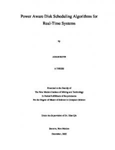
5 α=2.5 α=3 α=4 α=5

4.5 Spatial Reuse Ratio

Lemma 4: The maximum number of concurrent transmisˆ is upper bounded by N . sions Nmax in the hexagon H The proof of Lemma 4 is given in the Appendix. Theorem 3: The approximation ratio of the GGS algorithm is at most 3KN . ˆ which are Proof: Consider the links in subset Lk,q (H), ˆ the links with receivers located in the hexagon H. The number of time slots that an optimal scheduling algorithm needs to ˆ can satisfy the traffic demands of the links in subset Lk,q (H) Fmax k,q ˆ not be less than Nmax . Because L (H) is only a subset of the total wireless link set L, the number of time slots that an optimal scheduling algorithm needs to schedule all the links in L satisfies the following inequality:

4 3.5 3 2.5 2 1.5 1

5

10

15 SINR Requirement γ (dB)

20

25

0

Fig. 2.

Analytical Results of Spatial Reuse Ratio

GGS algorithm can be accomplished in O(|L| log2 |L| + K · 4 4 Ftotal · |L| ), which is equivalent to O(K · Ftotal · |L| ) time. This means GGS is a polynomial-time algorithm. The detailed proof is available in the online technical report [23]. VI. N UMERICAL AND S IMULATION R ESULTS In this section, we present numerical and simulation results of the GGS algorithm to gain further insights on how spatial reuse and power control influence the network performance. In our simulations, the transmitting nodes are uniformly distributed in a square area of 2000m × 2000m. The length of each link ranges from 10 to 50 meters. Each receiving node is randomly located between 10m and 50m from the corresponding transmitting node. Links’ traffic demands are uniformly distributed in the set [1, 3, 5, · · · , 19] with an average value of 10 time slots. We compare the performances of the following three algorithms: 1) AAS (existing algorithm): the Approximation Algorithm for the Scheduling problem proposed in [4]. 2) GS (our algorithm): the Guaranteed Scheduling part (lines 9 to 18) of Algorithm 1. 3) GGS (our algorithm): the complete Algorithm 1. In Fig. 2, we compare the spatial reuse ratio of the hexagon coloring in the GS algorithm with the square coloring in the AAS algorithm. Here the spatial reuse ratio is defined as the ratio of the smallest spatial reuse area in AAS (four squares) to the one in GS (three hexagons). Because the effects of the cumulative interference are treated differently in the two coloring schemes, the sides of the square and the hexagon are different even for the same values of α and γ0 . A large value of spatial reuse ratio means that our GS algorithm offers better performance (since it can accommodate more links within a given area). Fig. 2 shows the spatial reuse ratio as a function of the SINR requirements γ0 . Different curves represent different choices of path loss exponent α. We can see that the spatial reuse ratios are greater than 1 for γ0 ≥ 5dB and α ≥ 2.5, which are typical for wireless communications. Also, the spatial reuse ratio increases when γ0 increases or α decreases. This is the case where the separation among links must be larger to meet the SINR targets. For a fixed range of link length, although the areas of both squares and hexagons increase, the hexagons expand much slower which leads to a larger spatial reuse ratio.

1536 Authorized licensed use limited to: Chinese University of Hong Kong. Downloaded on August 26, 2009 at 23:05 from IEEE Xplore. Restrictions apply.

This full text paper was peer reviewed at the direction of IEEE Communications Society subject matter experts for publication in the IEEE INFOCOM 2009 proceedings.

Average Number of Time Slots

2500

AAS GS GGS

2000 1500 1000 500 0

5

10

15 SINR Requirement γ (dB)

20

25

0

Fig. 3.

Average Frame Lengths (the number of links= 500)

Spatial Reuse Ratio

2.2 analytical result number of links=500 number of links=1000 number of links=2000 number of links=4000

2 1.8 1.6 1.4 1.2

Fig. 4.

5

10

15 SINR Requirement γ0 (dB)

20

25

Spatial Reuse Ratio (Simulations v.s. Analysis) with α = 4

Fig. 3 shows the average frame lengths of these three algorithms as a function of SINR requirements γ0 . We simulate a wireless network with 500 links with α = 4. It is clear from Fig. 3 that GGS algorithm outperforms GS, which in turn outperforms AAS. The better spatial reuse demonstrated in Fig. 2 explains why GS is better than AAS. By adding a greedy power control component, GGS achieves further improvement over GS. The improvement becomes more significant when the SINR requirement increases. The average frame length of GGS grows much slower than GS and AAS with SINR target increase. At γ0 = 25dB, using AAS algorithm as the base line, GS achieves a frame length reduction of more than 50% and GGS achieves more than 80%. In Fig. 4, we compare the simulated performance ratio between GS and AAS with the theoretical results in Fig. 2. This is motivated by the fact that the two algorithms mainly differ in their coloring mechanisms (hence, the difference in their spatial reuse ratios). Under the assumption that α = 4, Fig. 4 shows that the trends of the simulated results closely follow the theoretical results. It also shows that the gap between the simulation and theoretical results becomes smaller when the network becomes denser. The gap is likely due to the fact that a link which could be scheduled in theory does not exist in practice. The probability of this happening decreases as the network becomes more dense. VII. C ONCLUSION We considered the joint power control and minimum-framelength scheduling problem in wireless networks, under the

physical interference model and subject to consecutive transmission constraints. We presented the first NP-completeness proof of this problem in the literature. Compared with the widely used protocol interference model, the physical interference model leads to more realistic (but also more complicated) characterization of wireless interference. We prove the NP-completeness by identifying a proper instance of our scheduling problem and reduce a well-known NP-complete problem (i.e., Partition Problem) to it. We then proposed the first polynomial-time algorithm with a bounded approximation ratio for the power controlled scheduling problem under the physical interference model. Both the algorithm and the approximation ratio are applicable for any network topology with or without consecutive transmission constraints. Through extensive simulations under various system parameters, we show that our algorithm outperforms the state-of-the-art algorithm in the literature, thanks to better spatial reuse and efficient power control. There are a number of challenging questions arising from the work in this paper. Although we successfully proposed a polynomial-time algorithm with bounded approximation ratio for the power controlled scheduling problem, the bound may be loose for some network settings. Finding a tighter bound would be an interesting problem. Another interesting direction is to develop a distributed scheduling algorithm based on our algorithm. We believe that the ideas and the theoretical results presented in this paper are very useful in designing distributed scheduling algorithm with bounded approximation ratio. A PPENDIX A P ROOF OF L EMMA 4 First we show that Nmax is upper bounded by N1 . We prove this by contradiction. Consider any two links li and lj in subset ˆ Since both the receivers Ri and Rj are located in Lk,q (H). ˆ we have the following two inequalities: the hexagon H, dmax dmax < d(Ti , Ri ) ≤ k−1 , k 2 2 dmax dmax d(Tj , Ri ) ≤ 2A + k−1 = (2W + 1) · k−1 . 2 2 So any non-zero element in the relative path gain matrix B satisfies the following inequality: −α  max (2W + 1) · 2dk−1 d−α (Tj , Ri ) 1 > =  d −α α. −α max d (Ti , Ri ) (2 (2W + 1)) k 2

Suppose N1 + 1 links can be active simultaneously. There are N1 non-zero elements in each row of the relative path gain matrix B. We can find that for any row, the row sum Srow satisfies the following inequality: 1 Srow > N1 · α (2 (2W + 1))

1 1 α · > (2 (2W + 1)) α γ0 (2 (2W + 1)) 1 = . γ0

1537 Authorized licensed use limited to: Chinese University of Hong Kong. Downloaded on August 26, 2009 at 23:05 from IEEE Xplore. Restrictions apply.

This full text paper was peer reviewed at the direction of IEEE Communications Society subject matter experts for publication in the IEEE INFOCOM 2009 proceedings.

According to Theorem 3 we find that 1 ρ(B) ≥ min(Srow ) > . γ0 So condition (4) can not be satisfied, which means N1 + 1 number of links can not be active simultaneously. This is contradictory to our assumption. So we have Nmax ≤ N1 .

(13)

Next we show that Nmax is also upper bounded by N2 . ˆ We have Consider any two links li and lj in subset Lk,q (H). the following four inequalities: dmax dmax 1, there is a minimum requirement on the distance between Ri and Rj : 1 dmax d(Ri , Rj ) > (γ0 α − 1) k , (γ0 > 1). 2 If Nmax number of links can be active simultaneously, according to Proposition 2, we know that any two links of these Nmax links can be active simultaneously. This means that the distance of any two receivers should be greater than 1 (γ0 α − 1) dmax . We know that all the receivers are located in 2k ˆ with side length A. [22] gives a tight upper the hexagon H bound on the number of nodes packed in a Jordan polygon with minimum distance requirement. The bound is related to both the area and the perimeter of the Jordan polygon. When applying the result in [22] to our problem, we have ⎥ ⎢  2   ⎥ ⎢ ⎥ ⎢ 2W 2W ⎣ Nmax ≤ 3 + 1⎦ , (γ0 > 1). +3 1 1 γ0α − 1 γ0α − 1 (18)

So Nmax is also upper bounded by N2 . According to (13) and (18), we know Nmax is upper bounded by the minimum of N1 and N2 : Nmax ≤ min{N1 , N2 } = N. R EFERENCES [1] S. A. Borbash and A. Ephremides, “Wireless link scheduling with power control and SINR constraints”, IEEE Trans. Information Theory, vol. 52, no. 11, pp. 5106-5111, Nov. 2006. [2] G. Brar, D. M. Blough, and P. Santi, “Computationally efficient scheduling with the physical interference model for throughput improvement in wireless mesh networks”, In Proceedings of ACM Mobicom, pp. 2-13, 2006. [3] G. Sharma, R.R. Mazumdar, and N.B. Shroff, “On the Complexity of Scheduling in Wireless Networks”, In Proceedings of ACM Mobicom, pp. 227-238, 2006. [4] O. Goussevskaia, Y.A. Oswald, and R. Wattenhofer, “Complexity in Geometric SINR”, In Proceedings of ACM MobiHoc, pp. 100-109, 2007. [5] T. Moscibroda and R. Wattenhofer, “ The Complexity of Connectivity in Wireless Networks.”, In Proceedings of the 25 th IEEE Infocom , 2006. [6] T. Moscibroda, Y. A. Oswald, and R. Wattenhofer, “ How optimal are wireless scheduling protocols? ”, In Proceedings of IEEE Infocom, Anchorage, Alaska, USA, May 2007. [7] T. Moscibroda, R. Wattenhofer, and A. Zollinger, “ Topology Control Meets SINR: The Scheduling Complexity of Arbitrary Topologies”, In Proceedings of ACM MobiHoc, pp. 310-321, 2006. [8] K. Jain, J. Padhye, V. Padmanabhan, and L. Qiu, “Impact of interference on multi-hop wireless network performance,” In Proceedings of ACM Mobicom, pp. 66-80, 2003. [9] R. Ramaswami and K. K. Parhi, “Distributed scheduling of broadcasts in a radio network,” In Proceedings of IEEE Infocom, 1989. [10] D. Chafekar, V.S. Kumar, M.V. Marathe, S. Parthasarathy, and A. Srinivasan, “Cross-layer Latency Minimization in Wireless Networks with SINR Constraints”, In Proceedings of ACM MobiHoc, pp. 110119, 2007. [11] P. Gupta and P.R. Kumar, “The Capacity of Wireless Networks,” IEEE Trans. Information Theory, vol.46, no. 2, pp. 388-404, Mar. 2000. [12] T. Moscibroda, R. Wattenhofer, and Y. Weber, “ Protocol Design Beyond Graph-Based Models”, In Proceedings of ACM SIGCOMM Workshop on Hot Topics in Networks (HotNets), 2006. [13] J. Chen, K. Sivalingam, P. Agrawal, and R. Acharya,“Scheduling multimedia services in a low-power MAC for wireless and mobile ATM networks”, IEEE Trans. Multimedia, vol. 1, no. 2, pp. 187-201, June 1999. [14] IEEE Std 802.16-2004, “IEEE Standard for Local and Metropolitan Area Networks—Part 16: Air Interface for Fixed Broadband Wireless Access Systems,” October 2004. [15] S. Even, O. Goldreich, S. Moran, and P. Tong, “On the NP-completeness of certain network testing problems,” Networks, 14: 1-24, 1984. [16] S. A. Grandhi, R. Vijayan, D. J. Goodman, and J. Zander, “Centralized power control in cellular radio systems”, IEEE Trans. Veh. Technol., vol. 42, no. 6, pp. 466-468, Nov. 1993. [17] R. A. Horn and C. R. Johnson, Matrix Analysis, New York: Cambridge Univ. Press, 1991. [18] S. A. Borbash and A. Ephremides, “The feasibility of matchings in a wireless network”, IEEE Trans. Information Theory, vol. 52, no. 6, pp. 2749-2755, Nov. 2006. [19] D. Mitra, “An asynchronous distributed algorithm for power control in cellular radio systems”, In Proceedings of 4th WINLAB Workshop, Rutgers University, New Brunswick, NJ, 1993. [20] N. Bambos, C. Chen, and G. Pottie,“Channel access algorithms with active link protection for wireless communication networks with power control”, IEEE/ACM Transactions on Networking, vol. 8, no. 5, pp. 583597, Oct. 2000. [21] M. R. Garey and D. S. Johnson, Computers and Intractability, A Guide to the Theory of NP-Completeness San Francisco, CA: Freeman, 1979. [22] Norman Oler, “A Finite Packing Problem”, Canad. Math. Bull. vol.4, no.2, May 1961. [23] L. Fu, S. Liew, and J. Huang, “Power Controlled Scheduling with Consecutive Transmission Constraints: Complexity Analysis and Algorithm Design,” Technical Report. http://www.ie.cuhk.edu.hk/∼jwhuang/ publication/Scheduling TechReport.pdf.

1538 Authorized licensed use limited to: Chinese University of Hong Kong. Downloaded on August 26, 2009 at 23:05 from IEEE Xplore. Restrictions apply.