Power domination in maximal planar graphs

Power domination in maximal planar graphs Paul Dorbec, Antonio Gonz´alez and Claire Pennarun

arXiv:1706.10047v1 [cs.DM] 30 Jun 2017

July 3, 2017 Abstract Power domination in graphs emerged from the problem of monitoring an electrical system by placing as few measurement devices in the system as possible. It corresponds to a variant of domination that includes the possibility of propagation. For measurement devices placed on a set S of vertices of a graph G, the set of monitored vertices is initially the set S together with all its neighbors. Then iteratively, whenever some monitored vertex v has a single neighbor u not yet monitored, u gets monitored. A set S is said to be a power dominating set of the graph G if all vertices of G eventually are monitored. The power domination number of a graph is the minimum size of a power dominating set. In this paper, we prove that any maximal planar graph of order n ≥ 6 admits a power dominating set of size at most n−2 . 4

1

Introduction

The notion of power domination arose in the context of monitoring an electrical network [1, 14, 15], i.e., knowing the state of each component (e.g. the voltage magnitude at loads) by measuring some variables such as currents and voltages. The measurements are done by placing Phasor Measurement Units (PMUs) at selected locations. PMUs monitor the state of the adjacent components, then with the use of electrical laws (such as Ohm’s and Kirschoff’s Laws), it is possible to determine the state of components further away in the network. Since PMUs are costly, it is important to monitor a graph with as few PMU as possible. In this paper, we consider the problem of monitoring maximal planar graphs with few PMUs. Before getting further into technical details, we need the following graph definitions. Let G = (V (G), E(G)) be a finite, simple, and undirected graph of order n = |V (G)|. The open neighborhood of a vertex u ∈ V (G) is NG (u) = {v ∈ V (G) | uv ∈ E(G)}, and its closed neighborhood is NG [u] = NG (u) S∪ {u}; the open and closed neighborhood of a subset of vertices S is NG (S) = v∈S NG (v) and NG [S] = S ∪ NG (S), respectively. The subgraph of G induced by S is written G[S] (the subscript G is dropped from the notations when no confusion may arise). The electrical network monitoring problem was transposed into graph-theoretical terms by Haynes et al. [9]. Originally, the definition of power domination ensured the monitoring of the edges as well as of the vertices, and contained many propagation rules. Here, we consider an equivalent definition from [3] that only requires monitoring the vertices. Given a graph G and a set S ⊆ V (G), we 1

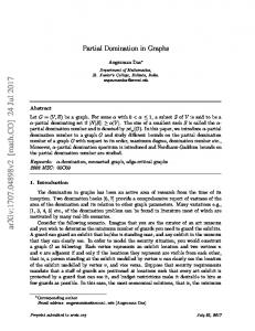
build a set MG (S) (or simply M (S) when the graph G is clear from the context) as follows: at first, MG (S) = N [S], and then iteratively a vertex u is added to MG (S) if u has a neighbor v in MG (S) such that u is the only neighbor of v not in MG (S) (we say that v propagates to u). At the end of the process, we say that MG (S) is the set of vertices monitored by S; the non-monitored vertices are those of the set V (G) \ MG (S). We say that G is monitored by S when MG (S) = V (G) and, in that case, S is said to be a power dominating set of G. The minimum cardinality of such a set is the power domination number of G, denoted by γP (G). The decision problem Power Dominating Set naturally associated to power domination (i.e., “Given a graph G and an integer k, does G have a power dominating set of order at most k?”) was proven NP-complete, by a reduction from the 3-SAT problem [9, 11] (giving NP-completeness of the problem on bipartite graphs, chordal graphs and split graphs). A reduction from Dominating Set was also given [8, 10], that implies the NP-completeness when restricted to planar graphs or circle graphs. However, polynomial algorithms were proposed to compute the power domination number of trees [9, 8], block graphs [16], interval graphs [11], and circular-arc graphs [11, 12]. Concerning the parameter γP (G), tight upper bounds are also known for particular classes: γP (G) ≤ n3 if G is connected [18] or a tree [9], whereas cubic graphs satisfy γP (G) ≤ n4 [4]. Furthermore, the exact value of γP (G) has been determined for regular grids and their generalizations: square grid [6] and other products of paths [5], hexagonal grids [7], as well as cylinders and tori [2]. The only known results for general planar graphs concern graphs with diameter two or three [17]. A graph G is a planar graph if it admits a crossing-free embedding in the plane. When the addition to G of any edge would result in a non-planar graph, G is said to be a maximal planar graph. A planar graph G together with a crossing-free embedding on the plane is called a plane graph, or a triangulation when G is a maximal planar graph. For any subset S ⊆ V (G), the graph G[S] can be viewed as a plane graph with the embedding inherited from the embedding of G. The only unbounded face is called the outer face of G, and the vertices of G are called respectively exterior or interior depending on whether they belong to the outer face or not. We say that a subgraph of a triangulation G is facial if all of its faces but the outer face are also faces of G. In particular, we denote by [uvw] a facial triangle formed by vertices u, v and w in G. Note that power dominating sets are independent of the embedding of the graph as they only depend on vertex adjacencies. We only make use of the embedding of the graph in the proofs. The main result of this paper consists in the following theorem: Theorem 1.1. If G is a maximal planar graph of order n ≥ 6, then γP (G) ≤ n−2 4 . The bound of Theorem 1.1 is tight for graphs on six vertices. We also know of one graph on ten vertices for which this bound is tight, the triakis tetrahedron drawn in Figure 1. To propose a general family of maximal planar graphs that have large power domination number, we use the configurations of Figure 2. Observe that if one of these configurations H is a facial subgraph of G, then 2

Figure 1: The triakis tetrahedron, having ten vertices and power domination number two. any power dominating set of G contains one of the vertices of H. Otherwise, even if all the exterior vertices are monitored, they can not propagate to any of the interior vertices of H. Thus γP (G) is at least the number of disjoint facial special configurations in G. Taking many disjoint copies of the two first configurations (that have six vertices) and then completing the graph into a triangulation by arbitrarily adding edges between external vertices of the configurations (see Figure 3), we obtain a family of graphs that have power domination number n6 . Note that this construction is similar to the construction for classical domination given in [13] reaching the bound γ(G) = n4 . As a consequence, and thanks to Theorem 1.1, we also get the following result: Theorem 1.2. For n ≥ 6, every maximal planar graph with n vertices has a power dominating set containing at most α(n) vertices, with n6 ≤ α(n) ≤ n−2 4 . Determining the best possible value of α(n) remains an open problem.

Figure 2: The good, the bad and the ugly configurations in a triangulation.

Figure 3: A class of maximal planar graphs for which γP (G) = hatched area is triangulated arbitrarily.

n 6.

The

The proof of Theorem 1.1 is done in three distinct steps, each of them described in a separate algorithm in Section 3. The first algorithm deals with the special configurations formed by overlapping configurations from Figure 2. 3

These special configurations are characterized in Section 2. The end of the proof relies on a final Lemma that is proved in Section 4.

2

Identifying bad guys

Our algorithm deals first with some special configurations, that are the possible intersections of the configurations from Figure 2. We here characterize these special configurations. Note that a facial octahedron (third configuration of Figure 2) may only share vertices of its outer face with other configurations. We thus focus on the other two configurations. We call 3-vertex a vertex of G with degree 3, and therefore whose neighborhood induces a K4 . A b-vertex is any vertex u ∈ V (G) with exactly two 3-neighbors v and v 0 , and such that N [u] = N [v] ∪ N [v 0 ]. Note that b-vertices have degree at most six and their neighborhood necessarily induces one of the subgraphs of Figure 4. In all figures of this section, b-vertices are depicted with blue squares, and 3-vertices are drawn white.

Figure 4: The two possible neighborhoods of a b-vertex v. Observation 2.1. Any two b-vertices u, u0 ∈ V (G) are adjacent if and only if there exists a 3-vertex v ∈ N (u) ∩ N (u0 ). Proof. By definition of b-vertices, if u0 is adjacent to u, it is also adjacent to a 3-vertex v adjacent to u, and so u and u0 have a common neighbor of degree 3. Moreover, if v has degree 3, all its of v are pairwise adjacent, and thus two b-vertices u and u0 that have v as a common neighbor are adjacent. Lemma 2.2. If G contains two 3-vertices v1 , v2 with two common b-neighbors, then G is isomorphic to one of the graphs depicted in Figure 5. Proof. Either v1 and v2 have three common neighbors (inducing the first subgraph), or they have distinct third neighbors (inducing the second subgraph). In the first subgraph, all triangles are incident to a 3-vertex, so they are facial and there is no possibility for more vertices in the graph. In the second subgraph, the only faces not incident to a 3-vertex are incident to a b-vertex, which can not have other neighbors. Again, all triangles must then be facial. Lemma 2.3. If all the neighbors of a 3-vertex are b-vertices, then G is isomorphic to a graph depicted in Figure 5 or these vertices belong to a facial triakis tetrahedron as depicted in Figure 6.

4

v1 v1

v2

v2 Figure 5: The two possibilities for G if two 3-vertices v1 and v2 have two common b-neighbors. In both cases, γP (G) = 1. Proof. Let v be a 3-vertex adjacent to three b-vertices u1 , u2 and u3 , which necessarily form a triangle. By definition of a b-vertex, each ui has another 3neighbor vi . If the vertices vi are not all distinct, then there exist two b-vertices sharing two adjacent 3-vertices, and Lemma 2.2 concludes. So assume the vi are distinct. Let w1 and w2 be the neighbors of v1 distinct from u1 (which are both adjacent to u1 ). Since u1 may not have any other neighbor, we infer without loss of generality that w2 is adjacent to u2 (and w1 to u3 ), and therefore that w2 is also adjacent to v2 (and w1 to v3 ). Similarly, v2 and v3 must have some vertex w3 as a common neighbor, also adjacent to u2 and u3 . Now, since the neighborhoods of 3-vertices and b-vertices are fully determined, we get a facial triakis tetrahedron, as depicted in Figure 6. w2

v2

v1 u1 v

u2 u3 v3

w3

w1

Figure 6: A facial triakis tetrahedron. Observe in particular that if a b-vertex has three adjacent b-vertices, then by Observation 2.1, we are in the case of Lemma 2.3 (and the graph is a triakis tetrahedron). Lemma 2.4. If G contains three b-vertices forming a three cycle, then either Lemma 2.3 applies, or G contains the first configuration depicted in Figure 7, or it is isomorphic to one of the last two graphs depicted in Figure 7. Proof. Let u1 , u2 , u3 be three b-vertices forming a cycle. If they have a common 3-neighbor, then Lemma 2.3 applies, so assume they do not. By Observation 2.1, every two of these vertices have a 3-vertex as a common neighbor, and they are distinct by hypothesis. Let v1 , v2 , v3 be the 3-vertices adjacent respectively to u1 and u2 , u2 and u3 , and u1 and u3 , and let z1 , z2 , z3 be the (not necessarily distinct) third neighbors of respectively v1 , v2 and v3 . Suppose two zi are distinct, say z1 and z3 , and observe that the neighbors of u1 are exactly 5

{u2 , u3 , v1 , v3 , z1 , z3 }. Therefore, if (u1 u2 u3 ) separates z1 from z3 , then z3 is adjacent to u2 and z1 is adjacent to u3 . Now, since u2 is a b-vertex, then v2 is adjacent to z3 and z1 , a contradiction. So [u1 u2 u3 ] does not separate any two zi and is facial. Moreover, if say z1 and z3 are distinct, then they must be adjacent since u1 has no other neighbor. So depending on whether the zi are distinct or not, G contains the first configuration depicted in Figure 7, or is isomorphic to one of the last two graphs depicted in Figure 7 (note that all faces incident to a 3-vertex or a b-vertex in these drawings are facial). z1 = z2 = z3

z1

z1 v1

v1

v1 u2

u1 v3 u3 z3

u1 u2

u1

v2

v3

u3

u2

v3

u3 v2

v2 z2 = z3

z2

Figure 7: The possible configurations of G if there is a face composed of b-vertices. The last two graphs, that satisfy γP (G) = 1, are contracts of the first configuration. Property 2.5. Let (u1 , u2 , u3 ) be a path on three b-vertices. Let v1 be the 3vertex adjacent to u1 and u2 and let v2 be the 3-vertex adjacent to u2 and u3 . If u1 is not adjacent to u3 , then there exist distinct vertices x and x0 such that {u1 , u2 , u3 , v1 } ⊆ N (x), {u1 , u2 , u3 , v2 } ⊆ N (x0 ), and [xu2 u3 ] and [x0 u1 u2 ] are facial (see Figure 8). Proof. Since v1 and v2 are 3-vertices, then there exist two vertices x, x0 such that {u1 , u2 , v1 } ∈ N (x) and {u2 , u3 , v2 } ∈ N (x0 ). Since u2 is a b-vertex, we have that x 6= x0 (otherwise u1 and u3 would be adjacent as the second configuration of Figure 4 shows). Thus, u2 is a b-vertex corresponding to the first configuration of Figure 4, and so x is adjacent to u3 , x0 is adjacent to u1 , and [xu2 u3 ] and [x0 u1 u2 ] are facial. x

u1

v1 u2 v2

u3

x0

Figure 8: There are two distinct vertices both adjacent to {u1 , u2 , u3 }. All triangles are facial.

6

Observe that the above property together with Lemmas 2.3 and 2.4 covers all possibilities of three connected b-vertices. We now consider the cases when b-vertices form paths and cycles of length at least four. Corollary 2.6. Suppose a set of k ≥ 3 b-vertices form a path (u1 , . . . , uk ) (where u1 and uk may be adjacent when k > 3). Let v1 , . . . , vk−1 be 3-vertices with vi being adjacent to ui and ui+1 , and let v0 be the 3-vertex adjacent to u1 but not to u2 . Then there exists a vertex x adjacent to all ui , 1 ≤ i ≤ k and to v0 and v2 . (see Figure 9). x

u1

v1 uk−1 uk

u2 v2 v0

x0

Figure 9: There are two vertices universal to the (u1 , u2 , u3 , . . . , uk ). Vertex x0 is also adjacent to v0 and v2 .

path

Proof. Applying Proposition 2.5 to vertices u1 , u2 , u3 , there exist distinct vertices x, x0 such that {u1 , u2 , u3 , v1 } ⊆ N (x), {u1 , u2 , u3 , v2 } ⊆ N (x0 ), and [xu2 u3 ] and [x0 u1 u2 ] are facial. Since x is adjacent to the b-vertex u3 , x must be adjacent to v3 and thus to u4 . Then u4 is also adjacent to x0 as u3 has no other neighbor. Iterating this argument, we infer that x and x0 are adjacent to all ui . Now, since x0 is adjacent to u1 but not to v1 , by definition of a b-vertex it is adjacent to v0 , and the corollary follows. Lemma 2.7. If G contains a maximal component of b-vertices isomorphic to P2 , then G contains a facial subgraph isomorphic to one of the graphs of Figure 10. Proof. Let u1 , u2 be b-vertices, and let v1 be the 3-vertex adjacent to u1 and u2 , and z the third neighbor of v1 . Let v0 and v2 be the second 3-neighbors of respectively u1 and u2 , which can be assumed distinct by Lemma 2.2. Since v0 is a 3-vertex and is not adjacent to u2 , v0 has a neighbor t which is adjacent to u1 and u2 (we can see u1 as the central vertex of any configuration of Figure 4). By definition of b-vertices, v2 must also be adjacent to t. Let z1 and z2 be the third neighbors of respectively v0 and v2 . If z1 = z2 , then N [t] ⊆ N [v0 ] ∪ N [v2 ], and the vertex t is in fact a b-vertex, contradicting our hypothesis. Thus z1 6= z2 . Depending on whether z and z1 are distinct or not, we get one of the configurations of Figure 10 (in both cases, the outer face of the drawing may not be facial).

7

z = z1

z

v0 u1

z1

z2

v1

z u1 v1 u2 2

u2 v0

v2 t

v2 t

Figure 10: The possible configurations of G if there is a P2 component of b-vertices. The outer faces are not necessarily facial. All other triangles of the drawing are facial. Finally, if there is an isolated b-vertex in G, then it belongs to one of the subgraphs depicted in Figure 4. This concludes the proof of the following lemma, that gives a characterization of the possible intersections of the configurations from Figure 2. The special configurations of G are then all the configurations depicted in Figure 11. Lemma 2.8. If G contains a special configuration as facial subgraph, then either G is a small graph (characterized in Lemmas 2.2, 2.3, and 2.4) and γP (G) ≤ n−2 4 , or each maximal component of b-vertices of G belongs to one of the induced configurations depicted in Figure 11, 1 to 7, or G contains a facial octahedron (configuration 8 in Figure 11). Observation 2.9. If a vertex belongs to two facial subgraphs isomorphic to configurations from Figure 11, then it is a vertex from the outer face for both of them. Proof. Let v be a vertex that belongs to two configurations of Figure 11. If v is a b-vertex, then none of the two configurations is an octahedron. Then by maximality of the components of b-vertices in each configuration, the two configurations must rely on the same set of b-vertices, so they are the same configuration. Now suppose v is a 3-vertex. In both configurations it must be an internal vertex, and have an adjacent b-vertex. So the configurations also share a b-vertex and the same argument concludes. Finally, if v is a vertex of degree 4, it is an internal vertex of an octahedron. Since two octahedra cannot intersect on internal vertices and no internal vertex of an octahedron may be adjacent to a 3-vertex, v does not belong to any other configuration. The observation follows.

3

Constructing the power dominating set

We now describe the process that defines incrementally a power dominating set S of G satisfying the announced bound. In Section 3.1, Algorithm 1 produces a set S1 monitoring special configurations from Figure 2 with a small number of vertices. Then, Algorithm 2 of Section 3.2 builds a set S2 by expanding the set S1 iteratively, while keeping certain properties. If the graph G is not fully monitored after that, we show in Section 3.3 that G has a characterized 8

2

1

3

6

4

5

7

8

Figure 11: The different configurations containing a b-vertex, and the octahedron. So-called “special” vertices of configurations 1 to 5 are circled in red. For these configurations, vertices circled with a blue-dashed curve form a set relative to the special vertex of the configuration, and they are called the circled vertices of the configuration. structure, which guarantees that our last Algorithm 3 maintains the wanted bound while adding some well chosen vertices to S2 to build the required set S. During the three algorithms, we ensure the following property on the set of selected vertices, that is necessary for the proof of Lemma 3.5: Property (∗). We say that a subset S of vertices of a plane graph G has Property (∗) in G whenever, for each induced triangulation G0 ⊆ G of order at least 4, if G0 is monitored by S then one of the following holds: (a) one vertex of the outer face of G0 has its closed neighborhood in G monitored by S, (b) or, we have |S ∩ V (G0 )| ≤

3.1

|V (G0 )|−2 . 4

Monitoring special configurations

The first step of our algorithm is described in Algorithm 1, which takes care of monitoring vertices creating special configurations. In the following, we say a configuration is monitored by S1 when all its interior b-vertices are in M (S1 ), or for an octahedron, if all its vertices are in M (S1 ). Note that the output of Algorithm 1 is the empty set whenever G contains neither b-vertices nor facial octahedra. We prove the following lemma: 9

Algorithm 1: Monitoring special configurations Input: A triangulation G of order n ≥ 6. Output: A set S1 ⊆ V (G) monitoring all b-vertices and all vertices of facial octahedra. S1 := ∅ if G has a vertex u of degree at least n − 2 then Label N [u] with u Return {u} if G is a triakis tetrahedron (as in Figure 6) then u, v: two b-vertices of G at distance 2 Label u, its 3-neighbors and two of its adjacent b-vertices with u Label all other vertices of G with v Return {u, v} while ∃ a non-monitored configuration H from Figure 11(1,2,3,4,5) do u: the special vertex of H S1 ← S1 ∪ {u} Label u and the circled vertices of H with u while ∃ non-monitored configurations H, H 0 from Figure 11(6,7,8) with a common vertex u do S1 ← S1 ∪ {u} Label u and the interior vertices of H and H 0 adjacent to u with u while ∃ a non-monitored configuration H from Figure 11(6,7,8) do u: any exterior vertex of H S1 ← S1 ∪ {u} Label all vertices of H with u Return S1

Lemma 3.1. Let S1 be the set obtained by application of Algorithm 1 to G. The following statements hold: (i) All b-vertices and all facial octahedra are monitored by S1 . (ii) If S1 is not empty, |S1 | ≤

|M (S1 )|−2 . 4

(iii) S1 has Property (∗) in G. Proof. (i) Every b-vertex in the graph belongs to one of the configurations of Figure 11. The selected vertices in each configuration monitor all the b-vertices of the configuration, and thus the algorithm monitors all such vertices. Taking any vertex of a facial octahedron monitors the whole octahedron, thus all facial octahedra are monitored as well. (ii) If the graph is dealt with by the first if s, the statement is straightforward. Otherwise, we first ensure that for each vertex u ∈ S1 , there are indeed at least five vertices labeled with u. For configurations 1, 3, 4 and 5, this is clear by definition of the circled vertices. For configuration 2, the vertex taken plus the (at least) three b-vertices of the path plus at least one 3-vertex make (at least) five labeled vertices. For every vertex u added in the second while loop, there are at least two vertices labeled with u in each of the two configurations, which together with u itself makes five vertices. For vertices added in the last while loop, at least six vertices are labeled with u each time. 10

Now, we show that each vertex receives at most one label during Algorithm 1. By Observation 2.9, only vertices on the outer face of some configuration may be labeled several times, and so in only two cases: they may receive their own label when they are themselves added to S1 , or they may receive a label during the last while loop if they are in a non-monitored configuration 6, 7 or 8 disjoint from all remaining non-monitored configurations. Since these last configurations are monitored by any vertex of their outer face, all vertices are labeled at most once. If S1 contains two or more vertices at the end of the algorithm, the statement is proved. If S1 is reduced to a singleton, since the chosen vertex is of degree at least five, the statement holds. (iii) Let G0 be an induced triangulation of G monitored after Algorithm 1. If |S1 ∪ V (G0 )| = 0, then Property (∗).(b) holds. Assume then |S1 ∪ V (G0 )| > 0. If there is a vertex v ∈ S1 such that some vertices labeled with v are not in G0 , then v is a vertex of the outer face of G0 and Property (∗).(a) holds. Otherwise, for every vertex v ∈ S1 ∩ V (G0 ), all vertices with label v (which are at least five as said above) are in G0 . If |S1 ∩V (G0 )| ≥ 2, then this is sufficient to deduce that Property (∗).(b) holds. Otherwise, we observe that the set of vertices bearing a same label u either does not form an induced triangulation or is of size at least six, so G0 contains at least six vertices and the statement also holds. In the following, S1 denotes the output of Algorithm 1 applied to the graph G. Note that we can now forget the labels put on vertices during Algorithm 1.

3.2

Expansion of S1

The next step consists in selecting greedily any vertex that increases the set of monitored vertices by at least four. We first make a small observation. In the following, the graphs of the form P2 + Pk (i.e., formed by two vertices both adjacent to all vertices of a path Pk ) for some k ≥ 1 are called tower graphs. Remark that the only maximal planar graphs of order n ≤ 6 are the complete graphs K3 and K4 , the graphs P2 + P3 and P2 + P4 , the octahedron, and the flip-octahedron (see Figure 12).

Figure 12: The maximal planar graphs of order n ≤ 6. Observation 3.2. Let G be a triangulation. Unless G is an octahedron or a tower graph P2 + Pk (for some k ≥ 1), one interior vertex of G has degree at least 5. Proof. Suppose G is not an octahedron or a tower graph. If G is a flipoctahedron (last configuration of Figure 12), then one of its interior vertices has degree five. Otherwise, by the preceding observation, G contains at least seven vertices. Suppose by way of contradiction that all interior vertices of G have degree at most 4. Denote by u the exterior vertex of G with maximum degree, v, w the other two exterior vertices of G, and u1 , . . . , uk the interior 11

neighbors of u (k ≥ 2 or G is K4 ), so that (vu1 . . . uk w) form a cycle. Without loss of generality, we assume that v is adjacent to no less vertices among u1 , . . . , uk than w is. Let ` be the maximum integer such that for all i ≤ `, ui is adjacent to v. Since G is not a tower graph, ` < k. Observe that since v is not adjacent to u`+1 , u` and v have a common neighbor t (that is neither u`−1 nor u) to make another face on the edge vu` . If ` > 1, then v, t, u, u`−1 and u`+1 make five neighbors to u` , a contradiction. So ` = 1 and since u2 is not adjacent to v, t 6= u2 . (Note that t 6= w or v would have only one neighbor among u1 , . . . , uk while w has at least two, contradicting our assumption.) Thus u1 has at least four neighbors: u, v, u2 and t. By our initial assumption, [u1 u2 t] is a facial triangle. Now if k ≥ 3, u2 also already has four neighbors so [u2 u3 t] form a facial triangle. But then t and u3 are already of degree four, so it is not possible to form another facial triangle containing the edge tu3 , a contradiction. So k = 2, and [u2 wt] is facial. But then we get an induced octahedron where the only non facial triangle is [vtw], in which adding a vertex would raise the degree of t to more than 4, a contradiction. This concludes the proof. Let us now proceed with the second part of the algorithm defining a power dominating set. Assume that after Algorithm 1, M (S1 ) 6= V (G). We now apply Algorithm 2 that builds a set of vertices S2 ⊂ V (G) by iteratively expanding S1 in such a way that each addition of a vertex increases by at least four the number of monitored vertices. Moreover, at each round, the vertex added to S2 has maximal degree in G among all candidate vertices. Algorithm 2: Greedy selection of vertices to expand S1 Input: A triangulation G of order n ≥ 6 Output: A set S2 ⊆ V (G) with |S2 | ≤ |M (S42 )|−2 S2 := Algorithm 1(G) M := M (S2 ) while ∃ u in V (G) \ S2 such that |M (S2 ∪ {u})| ≥ |M | + 4 do Select such a vertex u of maximum degree in G. S2 ← S2 ∪ {u} M ← M (S2 ) Return S2

We now prove the following lemma: Lemma 3.3. Let S2 be the output of Algorithm 2 applied to G. The following statements hold: (i) |S2 | ≤

|M (S2 )|−2 . 4

(ii) S2 has Property (∗) in G. Proof. (i) Let ` denote the number of rounds of Algorithm 2 (i.e., the number (i) of vertices added during the “while” loop). For 0 ≤ i ≤ `, we denote by S2 the (0) set of selected vertices after the i-th round of Algorithm 2 (where S2 denotes (i) the result of Algorithm 1 applied to G), and by M (i) the set M (S2 ) of vertices 12

(i)

monitored by S2 . The algorithm ensures that for all 0 ≤ i ≤ `−1, we have that (i) (i+1) (i) if S2 is not the empty set, then |S2 | = |S2 | + 1 and |M (i+1) | ≥ |M (i) | + 4. So, provided we can establish a base case (either for i = 0 or i = 1), Statement (0)

(i) holds by induction on `. If S2 (0)

and thus |S2 | ≤

|M (0) |−2 . 4

(0)

is not the empty set, then 1 ≤ |S2 | ≤

|M (0) | 6 ,

Otherwise, by Observation 3.2, the first vertex added (1)

to S2 is of degree at least 5 so |M (1) | ≥ 6. Thus this time |M 4 |−2 ≥ 1 = |S2 |, and the induction allows to conclude. (ii) Let G0 ⊆ G be an induced triangulation monitored by S2 after Algorithm 2. First assume G0 is isomorphic to a tower graph. Note that no vertex selected during Algorithm 1 is an interior vertex of a tower graph. Observe that for each interior vertex v of a tower graph, there exists an exterior vertex v 0 such that N [v] ⊆ N [v 0 ] and d(v 0 ) > d(v). Then at any given round i, Algorithm 2 would rather select v 0 instead of any interior vertex v, and thus no interior vertex of G0 is in S2 . Since G0 is monitored, then at least one of the exterior vertices of G0 (say u) is in S2 or has propagated to an interior vertex of G0 , so N [u] ⊆ M and Statement (a) of Property (∗) holds for S2 in G. If G0 is isomorphic to the octahedron or to the flip-octahedron, then one of the exterior vertices of G0 is in S1 thanks to Algorithm 1, and Property (∗).(a) also holds. Assume now that |V (G0 )| ≥ 6, and suppose that Property (∗).(a) does not hold for G0 . Then some vertices of G0 belong to S2 , and vertices of V (G0 ) ∩ S2 only monitor vertices of G0 (no propagation may occur from a vertex of the outer face of G0 ). Then the same proof as for (i) above restricted to G0 shows that Property (∗).(b) holds. This proves that Property (∗) holds for S2 in G. (1)

In the following, S2 denotes the output of Algorithm 2 on the graph G.

3.3

Monitoring the remaining components

After Algorithm 2, some vertices of the graph may still remain non-monitored. Algorithm 3 thus completes the set S2 into a power dominating set of G, while keeping the wanted bound. In order to succeed, we need to have a better understanding of the structure of the graph around these non-monitored vertices. More precisely, we show that the graph can be described in terms of splitting structures (see Figure 13): they are structures composed of a set C = {u1 , u2 , u3 } of three non-monitored vertices and of two associated triangulations G1 and G2 whose exterior vertices are monitored. We make use of the following lemma, that is proved in Section 4. We denote by M G (S) the set of vertices not monitored by S in G (i.e., V (G) \ MG (S)). Lemma 3.4. Let G be a triangulation, S a subset of vertices of G monitoring all b-vertices and facial octahedra. Let G0 an induced triangulation of G. If M G (S) ∩ V (G0 ) 6= ∅, and for any v ∈ V (G), |MG (S ∪ {v})| ≤ |MG (S)| + 3 (i.e., Algorithm 2 stopped), then G0 corresponds to one of the configurations depicted in Figure 13. Observe that the triangulations associated to a splitting structure may contain non-monitored vertices, in which case we can again apply the above lemma and deduce that they are in turn isomorphic to a splitting structure. If M (S2 ) = V (G), then by Lemma 3.3, S2 is a power dominating set of G vertices. Otherwise, Algorithm 3 recursively goes down to with at most n−2 4 13

G1

G2

u1

G1

u2 u1

G1 u2

u2

u1

u3

u3

u3 G2

G2

(a)

(b)

(c)

u3

G1

G1 u1

u2

u1

u2 G2

G2

(d) u1

(e) G2

u1

G1 u2

u3

G1

u3

u3

u2

G2

(f)

(g)

Figure 13: The seven different splitting structures and their associated triangulations G1 and G2 . White vertices are non monitored. All triangles are facial except for G1 and G2 .

14

splitting structures whose associated triangulations are completely monitored, in which case it adds a vertex to S to monitor the remaining vertices. Algorithm 3: Monitoring the last vertices Input: A triangulation G of order n ≥ 6 and an induced triangulation G0 ⊆ G 0 Output: A set S ⊆ V (G0 ) monitoring G0 and such that |S| ≤ |V (G4 )|−2 S ← V (G0 )∩Algorithm 2(G) if ∃ u 6∈ MG (S) then G1 , G2 ← triangulations associated to the splitting structure of G0 containing u S 0 ← Algorithm 3(G, G1 ) S 00 ← Algorithm 3(G, G2 ) S ← S 0 ∪ S 00 ∪ {u} Return S We now prove that after the addition of vertices during Algorithm 3, the wanted bound still holds. Lemma 3.5. Let G0 be an induced triangulation of G, and S a subset of vertices of G monitoring all b-vertices and facial octahedra. Let C be a splitting structure in G0 with G1 and G2 its associated triangulations. Let u be a vertex of C, and let S 0 denote the set S ∩ V (G1 ) and S 00 the set S ∩ V (G2 ). If G1 and G2 are monitored by S and S 0 and S 00 have Property (∗) respectively in G1 and G2 , then S 0 ∪ S 00 ∪ {u} has Property (∗) in G0 , and G0 is monitored. Proof. First recall that after application of Algorithm 2, any vertex in MG (S) has at most three non-monitored neighbors. Therefore, in the induced triangulation G0 , a vertex adjacent to a vertex in C may not be adjacent to vertices from another configuration C 0 in G, or it would have two non-monitored neighbors in C and two in C 0 , a contradiction. Thus if a vertex can propagate in G0 , then it can also propagate in G. We know that S 0 and S 00 have Property (∗) in repectively G1 and G2 , and so G1 and G2 both satisfy either Property (∗).(a) or (b). Since all exterior vertices of G1 and G2 have non-monitored neighbors, then in fact, G1 and G2 satisfy Property (∗).(b). Thus |S 0 | ≤ |V (G41 )|−2 and |S 00 | ≤ |V (G42 )|−2 . Remark that |V (G0 )| ≥ |V (G1 )| + |V (G2 )| + 2 in every splitting structure. After adding a vertex u ∈ C, we have: |S 0 ∪S 00 ∪{u}| ≤

|V (G1 )| − 2 |V (G2 )| − 2 |V (G1 | + |V (G2 )| |V (G0 )| − 2 + +1 = ≤ . 4 4 4 4

Moreover, the exterior vertices of induced triangulations of G0 all have only monitored neighbors (the exterior vertices of G0 excepted) and thus S 0 ∪S 00 ∪{u} has Property (∗) in G0 . To prove that the addition of one vertex of C is sufficient to monitor G0 , we consider different cases depending on the splitting structure. • For splitting structures (a), (b) and (c), adding u2 , then u1 and u3 are monitored by adjacency.

15

• For splitting structures (d) and (e), adding u1 , then u2 is monitored by adjacency, and then any vertex of the outer face of G1 or G2 propagates to u3 . • For splitting structures (f) and (g), adding u1 , then two exterior vertices of G1 propagate independently to the other two vertices of C. Thus G0 is monitored, which concludes the proof. We can now use Lemma 3.5 to prove by direct induction on the splitting structures that at the end of Algorithm 3, Property (∗) holds for S in G. Moreover, the proof of Lemma 3.5 shows that for the set S, G satisfies Property (∗).(b). Thus the output S of Algorithm 3 satisfies the wanted bound and the graph is completely monitored. We thus get the following corollary that concludes the proof of Theorem 1.1. Corollary 3.6. At the end of Algorithm 3, M (S) = V (G) and |S| ≤

|V (G)|−2 . 4

In the following section, we finally prove Lemma 3.4.

4

Defining splitting structures

This section is dedicated to the proof of Lemma 3.4. In the following, we work under the assumption of the lemma, i.e., we assume that the set S monitors all octahedra and b-vertices, and that the addition of any vertex v to S would extend the set of vertices monitored by S by at most three. Any vertex contradicting the second part of the assumption is called a contradicting vertex. For simplicity, when G and S are clear from context, we denote M = MG (S) and M = V (G) \ MG (S). As a direct consequence of the definition of power domination, we get the following observation: Observation 4.1. Let S be a set of vertices of G such that for every vertex v ∈ V (G), |MG (S ∪ {v})| ≤ |MG (S)| + 3. The following properties hold: (i) Each vertex of M has either zero, two or three non-monitored neighbors. (ii) Each vertex of M has at most 2 neighbors in M . (iii) For every vertex u ∈ M \S, there exists v ∈ M ∩N (u) such that N [v] ⊂ M (that propagated to u). We now make the following statement. Lemma 4.2. If v is of degree at least five, then for every two neighbors u1 and u2 of v, there exists a neighbor w of v adjacent to u1 or u2 , but not both, and the corresponding triangle [vui w] is facial. Proof. We partition the set of neighbors of v into two paths from u1 to u2 : a path (w10 , . . . , wk0 ) of length at least three (i.e., k ≥ 2) and another path (w1 , . . . , w` ), possibly empty. We have w10 6= wk0 . By way of contradiction, assume both w10 and wk0 are adjacent to both u1 and u2 . Contracting the 0 path (w10 , . . . , wk−1 ) into w10 and the path (u1 , w1 , . . . , w` ) into u1 , we get that 16

x1 u

G2 v

G1 x2

x3 w

Figure 14: The configuration for G0 containing a non-monitored component isomorphic to K3 . G1 and G2 are triangulations. All other triangles of the drawing are facial. u1 , u2 , v, w10 , wk0 induce a K5 in the resulting graph, contradicting planarity of G. Thus w10 is not adjacent to u2 (and [w10 u1 v] is facial) or wk0 is not adjacent to u1 (and [wk0 u2 v] is facial). Remark that Lemma 4.2 also holds when v is in M with at least two neighbors in M . Indeed, by Observation 4.1(iii), v has a neighbor v 0 that propagated to it. Then v 0 only has monitored neighbors, and two of them are also adjacent to v. Thus v has degree at least five, which is the hypothesis of Lemma 4.2. Lemma 4.3. Connected components of G[M ] are of order at most three. Proof. Let C be a connected component of G[M ]. By Observation 4.1(ii), each vertex of M has degree at most two in M , so C is a path or a cycle. Then adding any vertex of C to S would monitor all of C. Since we work under the assumption of Lemma 3.4, C is of order at most three. Thus each connected component of G[M ] is isomorphic to either K3 , P3 , P2 , or K1 . Lemmas 4.4, 4.5 and 4.6 deal successively with the first three cases, whereas Lemma 4.7 goes through the case where M is an independent set in the induced triangulation considered. Lemma 4.4. Let G and M satisfy the assumption of Lemma 3.4. If an induced triangulation G0 contains a component of G[M ] isomorphic to K3 , then G0 is isomorphic to the configuration depicted in Figure 14. Proof. Let C be a component of G[M ] isomorphic to K3 with V (C) = {x1 , x2 , x3 }. Let u be a vertex of M , adjacent to at least one of the vertices of C. We first consider the case when u has neighbors in M \ C. If u is adjacent to two vertices in C, then by Observation 4.1(i), u has exactly one neighbor in M \C, say v. Then M (S ∪{u}) ⊇ M (S)∪{x1 , x2 , x3 , v}, and u is a contradicting vertex. So u has only one neighbor in C, say x1 . Within the neighborhood of x1 , the path from x2 to x3 going through u must contain at least three interior vertices since u is not adjacent to x2 or x3 , so x1 is of degree at least five. Applying Lemma 4.2 on x1 , we get that a neighbor w of x1 is adjacent to x2 or x3 but not both. Since w is adjacent to two vertices in C, it has no other neighbors in M or the above case would apply. Hence, adding u to S, all

17

y G1

y w w G1 z x2

x1

x2

x1

z

x3

x3 w0

w0

z

0

G2

G2

z0

y0

Figure 15: The two possible configurations for G0 containing a nonmonitored component isomorphic to P3 . G1 and G2 are triangulations. All other triangles of the drawing are facial. neighbors of u in M get monitored, then w propagates to x2 or x3 which can in turn propagate to the last vertex of C. So u is a contradicting vertex. We assume now that any vertex of M adjacent to C has only vertices of C as neighbors in M . Note that such a vertex must be adjacent to at least two vertices in C. Let u be a common neighbor of x1 and x2 such that [ux1 x2 ] is facial (u exists since the edge x1 x2 is contained in exactly two facial triangles). By Lemma 4.2, there is a neighbor v of u that is adjacent to only one of {x1 , x2 } (say x1 ) and [uvx1 ] is facial. The vertex v must have a second non-monitored neighbor, that must be in C, so v is adjacent to x3 . Observe that the triangle [vx1 x3 ] must be facial. Otherwise, there is a vertex t 6= v such that [tx1 x3 ] is facial and t is separated from x2 by (vx1 x3 ). Then by Lemma 4.2, t has a neighbor t0 with only one neighbor among {x1 , x3 } also separated from x2 by (vx1 x3 ), and thus with only one non-monitored neighbor, a contradiction. Now, v and x3 have a common neighbor w outside the triangle [vx1 x3 ], such that [vwx3 ] is facial. By definition of v, we have w 6= x2 . We also have w 6= u or v would be of degree three contradicting Observation 4.1(iii). The cycle (uvx3 x2 ) separates w from x1 , so the second non-monitored neighbor of w (different from x3 ) must be x2 . Unless an additional edge uw form a facial triangle [uwx2 ], there is another neighbor of x2 that is separated from both x1 and x3 by the cycle (uvwx2 ), a contradiction. So u is adjacent to w in a facial triangle [uwx2 ]. In a similar way that we proved that [vx1 x3 ] is facial, we infer that [wx2 x3 ] is facial. By construction, [ux1 x2 ], [uvx1 ], [vwx3 ] are facial, and we proved [vx1 x3 ], [uwx2 ] and [wx2 x3 ] also are. If the triangle [x1 x2 x3 ] is facial, then the graph induced by the vertices u, v, w, x1 , x2 , x3 is a facial octahedron, contradicting the assumption of Lemma 3.4. Thus [x1 x2 x3 ] is not facial, and applying the same line of reasoning as above inside [x1 x2 x3 ] shows that G0 is isomorphic to the configuration depicted in Figure 14. Lemma 4.5. Let G and M satisfy the assumption of Lemma 3.4. If an induced triangulation G0 contains a component of G[M ] isomorphic to P3 , then G0 is isomorphic to one of the splitting structures depicted in Figure 15. Proof. Let C be a component of G[M ] isomorphic to P3 with V (C) = {x1 , x2 , x3 }. 18

Let u be a vertex adjacent to C. We first prove that all neighbors of u in M are vertices of C. By Observation 4.1(i), u has at most two neighbors in M \ V (C). If u has exactly one neighbor u1 in M \ V (C), then x2 is a contradicting vertex, since u propagates to u1 once x2 is added to S. Assume then that u has two neighbors in M \ V (C) and thus only one neighbor in C. If u is adjacent to x1 or x3 , then u is a contradicting vertex. Suppose that u is adjacent to x2 only, which must then be of degree at least five. We apply Lemma 4.2 on x2 and get a neighbor v of x2 adjacent to x1 or x3 but not both. Taking u in S, v then propagates (and then x2 propagates to x3 ) so u is a contradicting vertex. Thus neighbors of C may not be adjacent to vertices in M that are not in C. We now prove that there is no vertex of M adjacent to all vertices of C. Suppose by way of contradiction that u is a vertex in M adjacent to x1 , x2 and x3 . By Lemma 4.2, u has a neighbor z ∈ M with exactly one neighbor in {x1 , x3 } (say x1 ) and [uzx1 ] is facial. Note that by the above statement, z is also adjacent to x2 . Again, we can apply Lemma 4.2 to find a neighbor z 0 of z adjacent to x1 or x2 but not both. Vertex z 0 must have a second non-monitored neighbor, namely x3 . So z 0 cannot be adjacent to x1 which is separated from x3 by (ux2 z), so z 0 is adjacent to x2 and x3 and [x2 zz 0 ] is facial. Now u is necessarily adjacent to z 0 forming a facial triangle [ux3 z 0 ] (otherwise some vertex would have a single neighbor in C). Observe that the triangle [zx1 x2 ] must be facial. Otherwise, there is a vertex t 6= z such that [tx1 x2 ] is facial and t is separated from x3 by (zx1 x2 ). Then by Lemma 4.2, t has a neighbor t0 with only one neighbor among {x1 , x2 } also separated from x3 by (zx1 x2 ), and thus with only one non-monitored neighbor, a contradiction. With a similar argument, we get that [z 0 x2 x3 ], [ux1 x2 ] and [ux2 x3 ] are facial. But then x2 is a b-vertex (as in the bad configuration of Figure 2), a contradiction. Let w, w0 , z, z 0 ∈ M such that [x1 x2 w], [x1 x2 w0 ], [x2 x3 z], [x2 x3 z 0 ] are faces. By the above statement, all these vertices are distinct. Suppose that there is a neighbor u of x2 different from the above vertices. Vertex u has a second neighbor in C, say x1 . The cycle (ux1 x2 ) separates w or w0 from x3 , say w. By Lemma 4.2, w has a neighbor with exactly one neighbor in {x1 , x2 }, and that cannot be adjacent to x3 , a contradiction. Thus x2 has no other neighbor. Renaming vertices if necessary, we suppose [x2 wz] and [x2 w0 z 0 ] are facial triangles. Note that x1 or x3 must have another neighbor. Otherwise, w is adjacent to w0 andz is adjacent to z 0 , which implies that x2 is a b-vertex (as in the ugly configuration of Figure 2), a contradiction. Let y ∈ M be a neighbor of x1 such that [x1 wy] is facial. The second neighbor of y in C is necessarily x3 . Similarly, z has a neighbor z1 such that [x3 z1 z] is facial and adjacent to x1 and x3 . Note that z1 6= w or w would be adjacent to three vertices in C. Then y = z1 or the cycle (x3 ywz) would separate z1 from x1 . We prove with similar arguments that there is a vertex y 0 such that [x1 w0 y 0 ] and [x3 z 0 y 0 ] are facial. If y = y 0 , then G0 is isomorphic to the first splitting structure of Figure 15. Otherwise, suppose first that x1 has another neighbor t. It also has to be adjacent to x3 . Then applying Lemma 4.2 to t, we find a vertex adjacent to only one vertex in C, a contradiction. So y and y 0 are adjacent, and [x1 yy 0 ]

19

x3

x3

G1 w u1

x1

G2

x2 w0

G1 w

u1

v1

x2

x1 v2

u2

v1

w0

v2

G2

Figure 16: The two possible configurations of an induced triangulation G0 if G[M ] has a connected component isomorphic to P2 . G1 and G2 are triangulations. All other triangles of the graph are facial. and [x3 yy 0 ] are facial. Thus G0 is isomorphic to the second configuration of Figure 15. Lemma 4.6. Let G and M satisfy the assumption of Lemma 3.4. If an induced triangulation G0 contains a non-monitored component isomorphic to P2 , then G0 is isomorphic to one of the configurations depicted in Figure 16. Proof. Let C = {x1 , x2 } with x1 x2 ∈ E(G), and let w and w0 be the vertices such that [x1 x2 w] and [x1 x2 w0 ] are facial. Claim 1. There is exactly one vertex of M at distance 2 of C. Proof. Suppose there is no vertex of M at distance 2 from C. By Lemma 4.2, w has a neighbor t ∈ M adjacent to only one vertex among {x1 , x2 }. Then t has only one neighbor in M , which contradicts Observation 4.1(i). Thus there is a vertex of M at distance 2 from C. Suppose that there is u0 ∈ M \ V (C) neighbor of a vertex u ∈ N (C) and v 0 ∈ M \ V (C) neighbor of another vertex v ∈ N (C). Then u is a contradicting vertex (whether it is distinct from v or not). () Let x3 be the only vertex of M at distance 2 of C. Claim 2. The vertices adjacent to x3 are exactly the vertices of (N (x1 ) ∪ N (x2 )) \ {w, w0 }. Proof. Suppose there is a vertex w00 ∈ M, w00 6= {w, w0 } adjacent to x1 and x2 . The cycle(x1 x2 w00 ) separates x3 from either w or w0 , say w. By Lemma 4.2, there exists a vertex v adjacent to w and to only one vertex among {x1 , x2 }. By Observation 4.1(i), v has a second non-monitored neighbor, that cannot be x3 , which contradicts Claim 1. Thus w and w0 are the only common neighbors of x1 and x2 . Therefore, all vertices adjacent to only one of x1 and x2 (i.e., in N (x1 ) ∪ N (x2 ) \ {w, w0 }) are adjacent to x3 (and there is at least one such vertex). Suppose there exists some vertex v adjacent to x3 but not in N (x1 ) ∪ N (x2 ). Then v is in M or it has another neighbor x4 ∈ M \ {x1 , x2 , x3 }, and v is a contradicting vertex. Thus no vertex v ∈ V (G) \ (N (x1 ) ∪ N (x2 )) is adjacent to x3 . 20

We now prove that w and w0 are not adjacent to x3 . Suppose w is adjacent to x3 . By Lemma 4.2, w has a neighbor u1 adjacent to only one of {x1 , x2 } (say x1 ) such that [u1 x1 w] is facial. (Thus u1 is also adjacent to x3 and [wu1 x3 ] is facial, since it separates x3 from x1 and x2 .) Again by Lemma 4.2, u1 has a neighbor v1 in M adjacent to only one of {x1 , x3 }. Suppose first v1 is adjacent to x3 (and not to x1 ). Then v1 is also adjacent to x2 . Following Observation 4.1(iii), w has other neighbors in M different from u1 . So there is a vertex t such that [x2 tw] is facial, and since t is separated from x1 by (x2 v1 x3 w), t is adjacent to x3 . Applying Lemma 4.2 on t, we get a contradiction. So v1 is adjacent to x1 but not to x3 , and thus v1 = w0 (and w0 is not adjacent to x3 ). But x3 has degree at least three, so there is a vertex v2 adjacent to x2 and x3 . Again, [u1 x3 w], [v2 x2 w] and [v2 x3 w] must be facial. But then there is no vertex that may have propagated to w. Thus w and w0 are not adjacent to x3 . () Let us now consider the neighbors of x1 and x2 in M \{w, w0 }. Let (u1 , . . . , uk ) and (v1 , . . . , v` ) be the paths from w to w0 among respectively N (x1 ) ∩ M and N (x2 ) ∩ M . Since x3 has degree at least 3, then by Claim 2, k + ` ≥ 3. First observe that k and ` both are at most 2. Otherwise, say k ≥ 3, then by Claim 2, each ui is adjacent to x3 , and the triangles [ui ui+1 x3 ] are facial, in particular [u1 u2 x3 ] and [u2 u3 x3 ]. But then u2 contradicts Observation 4.1(iii). We thus have two cases: • k + ` = 3, say u1 is the only neighbor of x1 and v1 , v2 are the only two neighbors of x2 in M \ {w, w0 }. By Claim 2, u1 , v1 and v2 are neighbors of x3 . Moreover, since none of {w, w0 } is adjacent to x3 , u1 is adjacent to v1 and v2 . Also by Claim 2, triangles [u1 v1 x3 ], [v1 v2 x3 ] and [u1 v2 x3 ] are facial, and G is isomorphic to the first graph depicted in Figure 16. • x1 and x2 both have exactly two neighbors in M \ {w, w0 }. By Claim 2, u1 , u2 , v1 and v2 are neighbors of x3 . Again, u1 is adjacent to v1 and u2 is adjacent to v2 since neither w nor w0 is adjacent to x3 . Also by Claim 2, triangles [u1 v1 x3 ], [v1 v2 x3 ], [u1 u2 x3 ] and [u2 v2 x3 ] are facial and G is isomorphic to the second graph depicted in Figure 16. This concludes the proof. Lemma 4.7. Let G and M satisfy the assumptions of Lemma 3.4. If an induced triangulation G0 is such that M ∩ V (G0 ) is an independent set, then G0 is isomorphic to one of the splitting structures depicted in Figure 17. Proof. Let G satisfy the assumptions of the lemma. In this proof, we denote 0 M 0 the set M ∩ V (G0 ), and M the set M ∩ V (G0 ). 0

Claim 1. There exists a vertex u ∈ M 0 with only two neighbors in M . Proof. Suppose by way of contradiction that every vertex in M 0 with non0 monitored neighbors has exactly three neighbors in M . Note first that no two 0 vertices in M 0 have exactly two common neighbors in M , or they would be contradicting vertices. Hence, they share either one or three such neighbors. 0 Suppose first that all vertices in M 0 with a common neighbor in M have exactly one such common neighbor. We define an auxiliary graph H as follows: 0 the vertices of H are the vertices in M , and two vertices in H are adjacent 21

u1

x

G2

x

u0

u3

u2

u1

G1 z

w1

u3

u2 G1

y

z

v1

w1

y

v1

G2

Figure 17: The two possible configurations of an induced triangulation G0 if M ∩ V (G0 ) is an independent set. G1 and G2 are triangulations. All other triangles of the drawings are facial. if they have a common neighbor in G0 . Observe that from a planar drawing of G0 , we can easily build a planar drawing of H: we keep the position of the vertices, and for each edge (uv) in H, u and v have a common neighbor x in G0 and we can have the edge (uv) follow closely the edges (ux) and (xv) (that 0 would not create crossings since NG0 (x) ∩ M = 3). By our assumption that no 0 two vertices in M 0 have more than one common neighbor in M , the degree of 0 a vertex in H is precisely twice its degree in G0 . Since every vertex in M has 0 degree at least 3 and every vertex in M 0 has three neighbors in M , that implies that H has minimum degree at least 6. But this contradicts Euler’s formula for planar graphs. So there are at least two vertices u and v in M 0 with three common neighbors 0 in M , say x1 , x2 and x3 , forming a subgraph isomorphic to a K2,3 . Consider such five vertices, such that the subgraph G00 induced by the vertices within the outer face of the K2,3 does not contain the same structure. Denote x1 and x3 the exterior vertices (i.e., x2 is inside the cycle (x1 ux3 v)). Since x1 , x2 and x3 are pairwise non adjacent, there is another neighbor w of x2 in M 0 , which has 0 at least two other neighbors in M . By minimality of the selected K2,3 , now all 0 vertices in G00 that belong to M 0 and share a neighbor in M do share exactly one. Building the graph H on G00 the same way as above, we get a planar graph H where every vertex has degree at least six except for x1 , x2 and x3 that have respectively degree at least 2, 4 and 2. Therefore, we get that the sum of the degrees of the vertices in H is at least 6|V (H)| − 10, again a contradiction with Euler’s formula. This concludes the proof. () 0

Claim 2. If a vertex u of M 0 has degree 2 in M , then all the vertices of 0 0 0 M sharing a neighbor in M with u also have degree 2 in M . 0

Proof. Let u1 be a vertex of M 0 with two neighbors v1 , v2 in M . Suppose that there exists a vertex u2 in M 0 adjacent to v1 or v2 (say v1 ) and with degree 0 3 in M . If u2 is not adjacent to v2 , then u2 is a contradicting vertex. So assume 0 u2 is also adjacent to v2 and let v3 be the third neighbor of u2 in M . Applying Lemma 4.2 to vertex u1 , let t be a vertex adjacent to only one of v1 and v2 , say 0 v1 , and such that [u1 v1 t] is facial. There is another vertex adjacent to t in M . If this vertex is not v3 , then t is a contradicting vertex (as u1 propagates to v2 22

0

then u2 to v3 ). So t has only two neighbors in M , v1 and v3 . Now, every other vertex in the graph is separated from v1 , v2 or v3 by one of the three separating cycles (u1 v1 u2 v2 ), (tv1 u2 v3 ) and (tu1 v2 u2 v3 ). The monitored vertex u2 necessarily has more neighbors (by Observation 4.1(iii)). Suppose there is a neighbor of u2 in the cycle (tu1 v2 u2 v3 ). Then there is a neighbor w to u2 and v2 forming a face [u2 v2 w]. If w is not adjacent to v3 , 0 then w has some extra neighbors in M , and is a contradicting vertex (u1 propagates to v1 then u2 to v3 ). If w is also adjacent to v3 , by Lemma 4.2 it has a neighbor adjacent to only one of v2 and v3 , also separated from v1 by the cycle (tu1 v2 u2 v3 ), and the same argument applies. The same arguments apply also if u2 has neighbors in the other separating cycles. Thus there is no vertex 0 adjacent to v1 or v2 with degree 3 in M . This concludes the proof. () 0

Let u1 be a vertex of M 0 with exactly two neighbors in M , denoted x and z. By Lemma 4.2, there is a neighbor of u1 adjacent to only one of x and z, say u2 is adjacent to x but not z (and [xu1 u2 ] is facial). By Claim 2, u2 has only one 0 other neighbor in M , denote it y. Note that we now have the property (P): any 0 neighbor v ∈ M of x, y or z has at least two neighbors in {x, y, z} and is not 0 adjacent to any vertex of M \ {x, y, z}. Otherwise v would be a contradicting vertex. Consider the two paths from u2 to z that partition N (u1 ). Let w1 be the last vertex before z in the path that does not go through x (i.e., [u1 w1 z] is facial and w1 is not adjacent to x). Since u2 is not adjacent to z, then w1 6= u2 . By the above property (P), w1 is adjacent to y. Moreover, y may not have a neighbor separated from x and z by (u1 u2 yw1 ), so [u2 w1 y] is a facial triangle. Suppose first that x is of degree three, and let u3 denote its third neighbor, adjacent to both u1 and u2 . It has one other neighbor among y and z, say y. Observe that [u2 u3 y] is necessarily a facial triangle, and that by Claim 2, u3 is not adjacent to z. Since z is of degree at least 3, it has a neighbor v1 6= u3 such that [u1 v1 z] is facial. By property (P), v1 is adjacent to y. Now z has no other neighbor within the cycle (v1 yw1 z), or it would be a common neighbor to y and z, but applying Lemma 4.2 would lead to a contradiction. So w1 is adjacent to v1 , and [v1 w1 y] and [v1 w1 z] are facial triangles. In addition, y cannot have a neighbor separated from x and z by (u1 u3 yv1 ) so [u3 v1 y] is a facial triangle. Thus we are in the first configuration of Figure 17. Assume now that each of x, y and z have degree at least 4. Let u3 form a facial triangle with x and u2 . If u3 is adjacent to z, then the fourth neighbor of x is also adjacent to z. By Lemma 4.2, it has a neighbor adjacent to only one of x and z, which is separated from y by (u1 xu3 z), a contradiction. So u3 is adjacent to y forming a facial triangle [u2 u3 x]. By the same argument, we infer the existence of u0 and v1 , common neighbors of x and z and of y and z respectively, and that the corresponding triangles are facial. If x were of degree 5, then we would get similarly a contradiction applying Lemma 4.2 on u3 or u0 . By the same reasoning on y and z, we obtain the second configuration of Figure 17, which concludes the proof of Lemma 4.7. The results from the four Lemmas 4.4, 4.5, 4.6 and 4.7 conclude the section: after Algorithm 2, each induced triangulation of G is isomorphic to one of the graphs depicted in Figure 13.

23

References [1] T. Baldwin, L. Mili, M. Boisen, and R. Adapa. Power system observability with minimal phasor measurement placement. IEEE Transactions on Power Systems, 8(2):707–715, 1993. [2] R. Barrera and D. Ferrero. Power domination in cylinders, tori, and generalized petersen graphs. Networks, 58(1):43–49, 2011. [3] D. J. Brueni and L. S. Heath. The PMU placement problem. SIAM Journal on Discrete Mathematics, 19(3):744–761, 2005. [4] P. Dorbec, M. A. Henning, C. L¨owenstein, M. Montassier, and A. Raspaud. Generalized power domination in regular graphs. SIAM Journal on Discrete Mathematics, 27(3):1559–1574, 2013. ˇ [5] P. Dorbec, M. Mollard, S. Klavˇzar, and S. Spacapan. Power domination in product graphs. SIAM J. Discrete Math., 22(2):554–567, 2008. [6] M. Dorfling and M. A. Henning. A note on power domination in grid graphs. Discrete Applied Mathematics, 154(6):1023–1027, 2006. [7] D. Ferrero, S. Varghese, and A. Vijayakumar. Power domination in honeycomb networks. Journal of Discrete Mathematical Sciences and Cryptography, 14(6):521–529, 2011. [8] J. Guo, R. Niedermeier, and D. Raible. Improved algorithms and complexity results for power domination in graphs. Algorithmica, 52(2):177–202, 2008. [9] T. W. Haynes, S. M. Hedetniemi, S. T. Hedetniemi, and M. A. Henning. Domination in graphs applied to electric power networks. SIAM Journal on Discrete Mathematics, 15(4):519–529, 2002. [10] J. Kneis, D. M¨ olle, S. Richter, and P. Rossmanith. Parameterized power domination complexity. Information Processing Letters, 98(4):145–149, 2006. [11] C.-S. Liao and D.-T. Lee. Power domination problem in graphs. In Computing and Combinatorics, pages 818–828. Springer, 2005. [12] C.-S. Liao and D.-T. Lee. Power domination in circular-arc graphs. Algorithmica, 65(2):443–466, 2013. [13] L. R. Matheson and R. E. Tarjan. Dominating sets in planar graphs. European J. Combin., 17(6):565–568, 1996. [14] L. Mili, T. Baldwin, and R. Adapa. Phasor measurement placement for voltage stability analysis of power systems. In Proceedings of the 29th IEEE Conference on Decision and Control, pages 3033–3038, Honolulu, Hawaii, 1990. IEEE. [15] A. Phadke, J. Thorp, and K. Karimi. State estimation with phasor measurements. IEEE Transactions on Power Systems, 1(1):233–238, 1986.

24

[16] G. Xu, L.-Y. Kang, E. Shan, and M. Zhao. Power domination in block graphs. Theoretical Computer Science, 359(1):299–305, 2006. [17] M. Zhao and L.-Y. Kang. Power domination in planar graphs with small diameter. Journal of Shanghai University (English Edition), 11:218–222, 2007. [18] M. Zhao, L.-Y. Kang, and G. J. Chang. Power domination in graphs. Discrete Math., 306(15):1812–1816, 2006.

25