Power efficiency has become the most important consideration for many modern computing devices. .... efficiency of softw
Power Efficiency for Software Algorithms running on Graphics Processors Björn Johnsson, Per Ganestam, Michael Doggett and Tomas Akenine-Möller Lund University
Abstract Power efficiency has become the most important consideration for many modern computing devices. In this paper, we examine power efficiency of a range of graphics algorithms on different GPUs. To measure power consumption, we have built a power measuring device that samples currents at a high frequency. Comparing power efficiency of different graphics algorithms is done by measuring power and performance of three different primary rendering algorithms and three different shadow algorithms. We measure these algorithms’ power signatures on a mobile phone, on an integrated CPU and graphics processor, and on high-end discrete GPUs, and then compare power efficiency across both algorithms and GPUs. Our results show that power efficiency is not always proportional to rendering performance and that, for some algorithms, power efficiency varies across different platforms. We also show that for some algorithms, energy efficiency is similar on all platforms.
1. Introduction All kinds of computing devices, be it CPUs, GPUs, or integrated CPUs with graphics processors, face great challenges in terms of power efficiency. Transistor technology scaling will no longer provide the performance improvements that we are used to [KDK∗ 11]. One of the reasons for this is that when the supply voltage, and consequently the threshold voltage, of the transistor is reduced, the current leakage of the transistor increases exponentially [BC11]. This, in turn, means that the supply voltage cannot be reduced, and that future architectures will be limited by power instead of area. It is well known that the power consumption of an external memory access, e.g., to DRAM, is substantially higher than both floating-point (more than an order of magnitude) and integer (more than three orders of magnitude) operations [Dal09], and for CPUs, logic tends to use more power than caches [BC11]. In addition, moving data inside a chip is also becoming increasingly expensive, and starts to be a major part of power dissipation. Historically, we are used to the growth of memory bandwidth being slower than compute growth, but lately, the memory bandwidth growth has slowed down more [KDK∗ 11]. Recently, Esmaeilzadeh et al. [EBA∗ 11] have modeled multi-core speedup as a combination of single-core scaling, multi-core scaling, and device scaling, and predict that with a 22 nm technology process, 21% of the chip has to be powered off. When the technol-
←− graphics card
←− PCIe extender card
←−our custom card
Figure 1: We have built a power measurement station, which measures power on the PCI express bus (which can deliver up to 75 W) and on the graphics card’s two power connectors, which in this case can deliver up to 75+150 W. This sums to a max of 300 W. ogy scales down to 8 nm, more than half the chip has to be powered off. This under-utilization is called dark silicon. On top of this, current leakage also increases exponentially with the temperature of the chip [ZPS∗ 03]. All this indicates that the main optimization axis for the foreseeable future for any computing architecture is power. It should be clear that predicting power consumption of a
Johnsson et al. / Power Efficency for Software Algorithms
particular architecture is not an easy undertaking, and in fact, it may not always be meaningful, since power consumption also is a function of the program that runs on the architecture. However, optimizing for lower power consumption is very important, and there are opportunities for improving the power efficiency of future architectures by developing new hardware mechanisms to reduce power. This has been the focus of mobile graphics, which often has translated to algorithms for bandwidth savings [AMS03]. For GPUs, simulators can be used to model power and leakage [SLS04], and different low-level hardware optimization techniques can be developed and studied [SSL05]. Power gating techniques can also be used [WYCC11]. It is also possible to save energy by reducing the precision in the computations in the vertex shader unit [PLS08, PLS11a] and in the pixel shader cores [PLS11b]. If you are not in a position to make power-efficient hardware changes, another approach to reduce power consumption remains, namely, to develop power-efficient software. Koduri [Kod11] suggests that software developers should optimize for power as well, and in particular so for mobile devices. Some of the advice includes minimizing the frame rate and continuing to optimize the code of an application even if the frame rate goal has been reached. In this paper, we take a different approach to study power efficiency of software running on graphics processors. We have built a power measurement station, as shown in Figure 1, which measures power consumption directly on the PCIe bus and on the power connectors of discrete graphics cards. For integrated CPU and graphics processors, we measure directly at the battery connection (for mobile phones) or directly on the power connectors of the motherboard. Using our power measurement station, we have studied the power efficiency of algorithms that generate exactly or approximately the same result, and we compare the power consumption per frame with the time needed to render the frame. For example, one of our case studies uses different shadow algorithms. In our study, power consumption is measured on two different discrete graphics cards, on a CPU with integrated graphics processor, and on a mobile phone, and these have widely different power efficiency characteristics. We hope that our research will spark an increased interest in the power efficiency of graphics software, and as such, that it opens a new research area for the graphics community.
2. Methodology Our goal in this research is to measure power consumption on a number of different rendering algorithms running on several different types of graphics architectures. This includes discrete graphics cards from different vendors, integrated graphics on the CPU die, and inside a mobile phone. Some graphics architectures have built-in counters to estimate some kind of power draw, but not all architectures ex-
Figure 2: Our power measurement station, also seen in Figure 1, connected directly on the battery power connects on an iPhone 4S. pose those, and they tend to estimate different things anyway. Instead, we take another approach, which allows for a fairer comparison (at least between different discrete graphics cards, or between different mobile phones, etc). The general idea is to measure power draw on all incoming power sources. It suffices to measure the current of the power sources, since the voltages are constant, and due to the following relationship between power, P, voltage, U, and current, I: P = UI.
(1)
The units are watts (W or joules/second) for power, volts (V) for voltage, and ampere (A) for current. Note that energy is the integral of P over time. In addition, the dissipation power due to switching in CMOS is P = CU 2 f , where C is the capacitance, and f is the clock frequency. For discrete graphics cards, there are several sources of power, namely, the PCI express bus, which can deliver up to 75 W, and between 0 and 2 power connectors, where connectors with 6 pins can deliver up to 75 W, and 8-pin connectors can deliver up to 150 W. To measure all currents on these power sources, we have built a custom power measurement station, as shown in Figure 1. The currents from the PCI express bus is measured using an Ultraview PCIeEXT-16HOT expander card, which has test points for measuring the currents. On our custom card, we have four ACS710 Hall effect current sensors, which can measure currents up to 12 A. There are also two shunt current sensors that can accurately measure smaller currents of up to 1 A, which are useful for mobile phone measurements. In Figure 2, we show the setup when measuring power on a mobile phone.
Johnsson et al. / Power Efficency for Software Algorithms
All these currents are going to an A/D converter, and these are fed to an ARM Cortex-M3 processor that samples the currents at 40 kHz. The resulting sampled signals are sent via ethernet to a PC, which can show the currents in real time directly in a window, or save them to a file for later analysis (e.g., conversion to power and filtering). The power measurement station as described above can be used directly to measure the power consumption of discrete graphics cards. For mobile phones and for CPUs with an integrated graphics processor, this approach cannot be used directly since the graphics processor is not an isolated unit. For mobile phones, we decided to measure all (including, for example, the display) power consumption by measuring power draw at the battery connector inside the phone. This is not perfect, but it is hard to measure more accurately than that, and at least, no power consumption is missed with this methodology. Similary for CPUs with integrated graphics processors, we measure the power consumption on the 4-pin power connector, which supplies +12 V to the mother board. For both these architectures, we subtract the power consumption in some form of “idle” state in order to isolate the power consumption of the graphics processor. We define the idle power as measured power draw of our application without submitting any OpenGL API calls at all† . These differences in measuring methodology affects the comparability of the results across platforms. On the integrated platform and mobile phone, the idle memory power usage is removed, but the power for graphics usage of memory is included. For this reason, we compare the relative consumption of different algorithms on different platforms, but in general, we attempt to not draw too detailed conclusions from comparing power consumption of discrete graphics cards and mobile phones or CPUs with integrated graphics. The questions that we were interested in answering when starting this project include: 1. What are the power characteristics of different graphics algorithms solving the same problem on different graphics architectures?
3. Case Studies We have chosen two case studies to measure power consumption on. Both of these are commonly used in real-time rendering today. The first is simply rendering the scene from the eye, and the second is shadow rendering. Those are described in the subsequent subsections. All our algorithms have been written in OpenGL and some have been ported to OpenGL ES, since we want to test them on mobile phones as well. 3.1. Case 1: Primary Rendering It is likely that graphics hardware’s most common use case is to render a scene from the eye, i.e., to evaluate both primary visibility and shading. We have three different flavors of this case study, where lighting with 32 spotlights (without shadows) is included. The first is basic forward rendering (FR), where the triangles simply are submitted as vertex arrays, and lighting computed for non-culled fragments. Our second technique starts with rendering the scene only to the depth buffer, which is followed by a pass with the depth test set to GL_LEQUAL and lighting computed for each fragment with a loop over the light sources. This way of priming the depth buffer avoids expensive pixel shading for fragments that will not be visible in the final image. We call this method Z-prepass rendering (ZR). Finally, we use deferred rendering (DR), which starts by creating various G-buffers [ST90], e.g., one buffer for depth, one for the normal in world space, one for specular exponent, and one for the diffuse texture. Then, for each light source, we render a volume covering the region of influence of the spotlight, and accumulate the lighting to each affected pixel. For all primary rendering algorithms, we use the same camera path through the Sponza atrium with five Stanford dragons added. The Sponza atrium contains 224, 337 triangles and the dragons contain 100, 000 triangles each. Some frames from this animation can be seen in the middle left part of Figure 4.
2. Is energy directly proportional to frame time?
3.2. Case 2: Shadow Algorithms
3. What does the power consumption look like during an animation?
As our second case study, we have chosen three different shadow algorithms, namely, shadow volumes (SV) [Cro77], shadow mapping (SM) [Wil78], and variance shadow mapping (VSM) [DL06]. While the algorithms for case 1 (Section 3.1) all generate exactly the same result, our chosen shadow algorithms only generate approximately the same result. For example, the shadow volume algorithm generates pixel-exact shadows without anti-aliasing, while the quality of both shadow mapping techniques depends on the shadow map resolution. In addition, variance shadow mapping provides filtered shadow lookups, and so has smoother edges. We chose those three shadow algorithms because they are rather different, and our hypothesis was that they may have different power consumption characteristics.
4. What does the power consumption look like inside a frame (for different algorithms)? 5. Can power optimization of software algorithms become a new subtopic in graphics? In the following, we will attempt to answer these questions.
† The CPU power cost of the OpenGL calls is included in the CPU with integrated graphics and mobile phone measurements.
Johnsson et al. / Power Efficency for Software Algorithms
The shadow map and variance shadow map algorithms need to render a shadow map — containing depths to the closest surfaces as seen from the light source — of the shadow casting geomety in a first pass. The variance shadow map algorithm then creates two mipmap hierarchies containing filtered depths, and filtered squared depths. Using Chebyshev’s inequality and those two mipmap hierarchies, the shadow test provides a floating-point value, instead of a binary outcome. Normal shadow maps do not use a mipmap hierarchy, and so gain some speed there. However, when the filter is large, variance shadow mapping will go up towards the tip of the mipmap hierarchy. For mipmap-based algorithms [Wil83], this is known to increase cache hit ratio as compared to not using a mipmap. As a result, the memory bandwidth usage to main memory is reduced. So even though variance shadow maps create a mipmap hierarchy, it is not clear that it will be more expensive in terms of power consumption. For the shadow algorithms, we use a camera path over the scene with tesselated geometry without textures. The scene contains 396, 344 polygons. Some frames from this animation can be seen in the middle right part of Figure 4.
3.3. OpenGL ES For the mobile phone, we use OpenGL ES, and there we have chosen to omit deferred rendering (DR), shadow volumes (SV), and variance shadow mapping (VSM). Deferred rendering was omitted since our target mobile platform does not support multiple render targets. A multi-pass solution for creating the G-buffers would be possible, but would not result in a fair comparison. Likewise, variance shadow maps were omitted, since it was not possible to implement without adding an extra pass. Shadow volumes were omitted because the mobile phone could not support the amount of geometry of our test scene without drastically splitting up geometry into more draw calls, which would incur a significant overhead.
Single Frame Rendering Signature Power Start Finish
300 Power (W)
The shadow volume algorithm extracts a shadow volume from each shadow caster by determining which of its edges are silhouette edges as seen from the light source. These edges are then extruded away from the light source, creating the sides of the shadow volume as quads. This shadow volume is then capped at each end. These shadow primitives are rasterized from the eye, and front facing quads increment the stencil buffer, while back facing quads decrement the stencil buffer. We have used Carmack’s reverse (also called z-fail) [AMHH08], where the increment/decrement is done for occluded shadow quads. Since a shadow quad often can cover many pixels, the shadow volume algorithm is known to burn fill rate.
250 200 150
29.4
29.45 Time (s) 29.5
29.55
Figure 3: Power signature of eight frames of forward rendering on the AMD Radeon 7970, where the fourth frame is followed by a delay which also affects our time stamp measurements.
4. Results Using our two case studies and our power measurement station, we have measured power on a series of GPUs. Starting with high-end discrete GPUs, we have taken measurements on an AMD Radeon HD7970 and on an NVIDIA GeForce GTX 580. For integrated GPUs, we measure power on an Intel Sandy Bridge Core i7 2700K with Intel HD 3000 graphics. The graphics processor part of Sandy Bridge is running at between 850 MHz and 1350 MHz because we have turbo mode enabled. In addition, we have set idle turbo mode to “high performance.” For mobile GPUs, we measure power on an iPhone 4S, which contains an Apple A5 chip with a dual core PowerVR SGX543MP2 GPU running at 250 MHz. In all main diagrams, we show the raw data, which often is a bit noisy, in a lighter color, while we show a low-pass filtered version with a fatter curve using a stronger color. In Figure 4, we show power consumption diagrams for both the GeForce 580 and the Radeon 7970 for our primary rendering application and for our shadow algorithms. These animations were rendered at 2560 × 1440 pixels. It should be noted that the GeForce was manufactured in 40 nm, while the Radeon was manufacted in 28 nm, which gives a power advantage for the Radeon.‡ This advantage is one of the possible reasons that Radeon power varies between 170–245 W, while GeForce power varies between 240–310 W. For the shadow algorithm runs, the number of lights is varied from 2 to 8 lights in increments of 2, and the resolution of the shadow maps was set to 25602 pixels. As can be seen, the Radeon 7970 has spikes where the frame time increases and, as a result, the average frame power decreases ‡ In all fairness, it should be noted that NVIDIA recently released the Kepler architecture [NVI12], which also is manufacted in 28 nm, and has been optimized for power (e.g., tripling the number of shader cores while lowering the shader core clock frequency). However, at the time of writing no such cards were available to us.
Johnsson et al. / Power Efficency for Software Algorithms
GeForce GTX 580
Primary Rendering Power and Frame Rendering time vs Frame Number
320
60
300
300
280
2 lights
4 lights
60
6 lights
8 lights
280 50
260
50
260 240
40 Rendering time (ms)
200 Power (W)
180 160
30
140 120
20
100
220
40
200
Rendering time (ms)
220
180
Power (W)
240
160
30
140 120
20
100
80
80
60
60
10
40
10
40
20 0 0
Shadow Algorithms Power and Frame Rendering time vs Frame Number
320
20 200
400 FR power
600 ZR power
800 1000 Frame Number DR power
FR time
1200 ZR time
1400
0 0
500
DR time
SV power
AMD Radeon HD 7970
Primary Rendering Power and Frame Rendering time vs Frame Number
260
1600
0
60
240 50
SM power
1500 Frame Number
VSM power
SV time
2000 SM time
2500
2 lights
4 lights
0
VSM time
Shadow Algorithms Power and Frame Rendering time vs Frame Number
220 200
220
1000
60
6 lights
8 lights
50
180
200 160
Rendering time (ms)
160 Power (W)
140
30
120 100
20
80
40
140
Rendering time (ms)
40
120
Power (W)
180
30
100 80
20
60
60 10
40
10
20
20 0 0
40
200
400 FR power
600 ZR power
800 1000 Frame Number DR power
FR time
1200 ZR time
1400
1600
0
DR time
0 0
500 SV power
1000 SM power
1500 Frame Number
VSM power
SV time
2000 SM time
2500
0
VSM time
Figure 4: Frame times and power consumption for primary rendering (left) and the different shadow algorithms (right) on an NVIDIA GTX580 (top) and on an AMD Radeon HD 7970 (bottom). Abbreviations: FR (forward rendering), ZR (Z-prepass), DR (deferred), SV (shadow volumes), SM (shadow mapping), and VSM (variance shadow mapping).
at the same time, as a longer period of idle power is taken into account. Looking at the frames in which this occurs, we see that the power usage does not really change compared to neighboring frames, but the time stamps for start and end of a frame are further apart as shown in Figure 3. At this point, we do not know the root cause of this, but since the frame
time increases, and those measurements are independent of our power measurement station, we are certain that it is not a shortcoming of our custom card. For primary rendering, FR is more expensive in terms of power on both platforms. On the GeForce 580, DR generally uses the least power, and has the best performance. On the Radeon 7970, ZR has higher
Johnsson et al. / Power Efficency for Software Algorithms
frame times than FR and DR at times, while FR and DR have about the same. For power, FR clearly uses the most power, while ZR and DR are more similar, but ZR often uses a little less power than DR. So even though FR and DR are generally faster, ZR uses less power. From these measurements, it is clear that one cannot just measure frame times in order to find the most energy-efficient algorithm (since FR and DR have about the same frame times, but widely different power usage, for example). For the shadow rendering results, the order of power usage is SV (highest), VSM, and then SM (lowest) for both discrete GPUs. Increasing the number of lights has little impact on power, except when going from 2 lights to 4 lights. In particular, on the Radeon 7970 when going from 2 to 4 lights, there is a large increase in SM power, but little change in SM frame times, and in fact, frame time goes down. The Radeon 7970 has two power states, where the first runs at 300 MHz and the second at 925 MHz. It would appear that SM with 2 lights runs at the 300 MHz state and then switches to the 925 MHz state for 4 lights. We cannot determine this exactly because we do not have accurate frequency measurements. Shadow performance on the GeForce 580 is clearly separated with SM being fastest, followed by VSM and then SV. Power consumption is clearly lowest for SM. On the Radeon 7970, SM is again the fastest, but SV and VSM vary over the animation with VSM varying a lot and SV staying fairly steady. The power measurements for the Sandy Bridge, which is manufactured in 32 nm, are shown in Figure 5, where the animation was rendered at 1600 × 1200 to reach real-time frame rates. The shadow maps for the Sandy Bridge measurements were scaled with a factor taking into account the difference in screen resolution, i.e., scaled by k = 1600 × 1200/(2560 × 1440) compared to the discrete GPUs. This means that we used 17922 as resolution for the shadow maps, and this is to make the energy/pixel measurements in Table 1 fairer. As can be seen, the power consumption for graphics varies between 8–22 W, and it contains a regular oscillation, which we presume is the effect of some voltage and frequency scaling. This oscillation originates in the idle power measurement, where the pattern is inversed. In general, we observed an idle power draw of about 40 W. The power results show that FR draws the most power followed by DR and ZR. The order of DR and ZR is the opposite compared to the GeForce 580, and yet the performance results show that DR is the fastest, then ZR and FR, which is the same order as the GeForce 580. This shows that performance is not always a good indicator of power and that it varies across platforms. We also note that both ZR and DR uses about 50% of the power of FR, and since ZR and DR also are faster, this turns into a significant difference in energy efficiency as we will see later (Table 1). For shadows, the power draw is highest for VSM, followed by SV. SM uses less power for only 2 lights, but then generally matches SV. This is quite different compared to the discrete cards in
that SV and VSM have changed places, and we note that SV on Sandy Bridge uses consistently less power than VSM. Shadow performance on Sandy Bridge has similar curves for each algorithm as the GeForce 580, with SM being the fastest, followed by VSM, and then SV. In Figure 6, we show the power measurements for the iPhone 4S, where the animation was rendered at 960 × 640. The shadow map resolutions were scaled in a similar manner as done for Sandy Bridge, resulting in a resolution of 10242 for this architecture. In general, the power consumption for graphics varies between 0.7–1.1 W. The power results show that ZR uses more power than FR to achieve lower frame times for ZR compared to FR. Again, we observe that frame time does not correlate to power usage, and it is only through power measurement analysis that the lower power algorithm can be determined. It is interesting to note that the iPhone uses a sort-middle architecture with deferred rendering [Ima11], which essentially performs a pre-Z pass in hardware before shading, and yet our ZR, which adds another pre-Z pass, still improves performance. SM runs at a much lower frame time than primary rendering due to the shadow scene having less geometry, but SM still uses more power for each frame. It is also interesting to compute how much energy is used over an entire animation divided by the number of frames in the animation and the screen resolution. This is computed as shown below: Z ttot
P(t)dt E=
0
F ·R
,
(2)
where ttot is the total time it took to render the entire animation, F is the number of frames in the animation, and R is the screen resolution in pixels. By dividing with screen resolution, we weigh in that different resolutions are used for different platforms. Two advantages of this measure are that GPUs that are faster to render the animation will integrate over a shorter time domain (ttot ), which should be taken into account, and that it is a screen resolution independent measure. We believe this makes the comparison fairer. In Table 1, we have gathered statistics for the average energy per pixel and its standard deviation. We note that in some situations, performance/Watt is reported. This could be interpreted as frames per second per Watt, which is frames per joule, and due to the resolution differences, we would report pixels/joule. While all the information is available in the table, we have chosen joules per pixel for the same reasons that frames per second often is avoided, and pure time per frame is preferred. One of these reasons is that one cannot split the running time of an algorithm into different parts and measure them using frames per second, while on the other hand, it makes sense to measure the time of a certain part of an algorithm. For power efficiency, we foresee a future where it may be possible to measure the power consumption for
Johnsson et al. / Power Efficency for Software Algorithms
Intel HD Graphics 3000 (Sandy Bridge) Primary Rendering Power and Frame Rendering time vs Frame Number
30
400
Shadow Algorithms Power and Frame Rendering time vs Frame Number
30
400
360 25
360 25
320
320
280 20
280 20
200
Rendering time (ms)
15
240
Power (W)
Power (W)
Rendering time (ms)
240
15
200
160 10
160 10
120
120
80 5
80 5
40
0 0
200
400
FR power
600
800 1000 Frame Number
ZR power
DR power
FR time
1200
ZR time
1400
1600
0
DR time
40
0 0
500
SV power
1000
SM power
Frame Number VSM power
1500
SV time
2000
SM time
2500
0
VSM time
Figure 5: Frame times and power consumption for primary rendering (left) and the different shadow algorithms (right) on an Intel Sandy Bridge integrated graphics HD3000.
a certain part of an algorithm, and therefore, joules/pixel is chosen in our presentation. Table 1 shows that energy/pixel follows similar trends across all GPUs. For primary rendering, it is noticeable that the differences between algorithms are much greater for the GeForce 580 and the Sandy Bridge than the Radeon 7970. For the shadow algorithms, we observe that SM, which uses a lighter rendering load, has similar energy/pixel over all four GPUs. However, it is also interesting to note that there is about an order of magnitude in difference in frame times (discrete GPUs are fastest), while at the same time there is more than an order of magnitude in difference in the number of transistors used for graphics (discrete GPUs use the most transistors). Also VSM, compared to SM, requires a small energy/pixel increase on the GeForce 580, but requires a more significant increase on the Radeon 7970 and on the Sandy Bridge. While SV, compared to VSM, has a large energy/pixel increase on the GeForce 580 and on the Sandy Bridge, but requires a small increase on the Radeon 7970. Our power measuring station samples at a high frequency, so we can look at the characteristics of individual frame power usage. Figure 7 shows frames for the GeForce 580 and Figure 8 shows frames for the Radeon 7970. For the primary rendering algorithms, FR shows full power usage throughout the frame, while ZR has some drops in power usage. DR shows a drop to idle power in the middle of the frame before finishing with full power usage. The shadow rendering algo-
rithm frames have 6 lights and the processing for the 6 lights can be clearly seen in each graph. It is interesting to note that in SM, both discrete cards drop to idle power between some lights, but for VSM only Radeon 7970 drops fully to idle, and does that between each light. Also, the amount of idle-time is larger for Radeon 7970.
5. Conclusions and Future Work Power is a major concern for all graphics processors today, and will be even more important in the future when technology continues to scale down. In this work, we have built a power measurement station, and measured power and frame times for a set of different GPUs and graphics algorithms. As we have shown, the fastest algorithm is not always the least power hungry algorithm, and we have also shown that this varies greatly between different architectures. More importantly, we believe that power is so incredibly important that it will become an integral part of most graphics research papers in the near future. We speculate that it will become as common to report joules per pixel as it is to report milliseconds per frame today. At this point, we have not provided any new and more energy-efficient algorithms. So, for future work, we want to focus on studying more algorithms, and to explore optimizations for existing algorithms that reduce power consumption, or even invent new algorithms with better power behaviour.
Johnsson et al. / Power Efficency for Software Algorithms
iPhone 4S
Primary Rendering Power and Frame Rendering time vs Frame Number
3000
1.2
2700
1.1
1.3
Rendering time (ms)
2100
0.8
Power (W)
1800
0.7
1500
0.6
1200
0.5 0.4
900
0.3
600
0.2
300
0.1 200
400 FR power
600
800 1000 Frame Number ZR power
1200
FR time
1400
1600
0
1200
6 lights
8 lights
1.1
900
1 0.9 0.8
Power (W)
0.9
4 lights
1.2
2400
1
2 lights
Rendering time (ms)
1.3
0 0
Shadow Algorithms Power and Frame Rendering time vs Frame Number
3300
0.7
600
0.6 0.5 0.4
300
0.3 0.2 0.1 0 0
ZR time
500
1000
1500 Frame Number
SM power
2000
2500
0
SM time
Figure 6: Frame times and power consumption for primary rendering (left) and the different shadow algorithms (right) on an iPhone 4S. Note that the frame time axis is different in the two graphs.
FR
Average energy/pixel (nJ) [std. dev] Primary rendering Shadow algorithms ZR DR SV SM VSM
GeForce 580 Radeon 7970
1443 [180] 607.4 [73.0]
722.1 [62.1] 510.6 [87.1] 1325 [114] 512.0 [103] 489.2 [79.9] 953.9 [44.9]
446.6 [80.3] 469.0 [88.3]
532.0 [67.5] 804.0 [250]
Sandy Bridge iPhone 4S
871.5 [134] 2234 [423]
314.2 [46.8] 280.0 [53.4] 2015 [290] −−−
311.3 [76.2] 460.5 [135]
511.3 [87.9] −−−
1317 [212] −−−
Table 1: Average energy per pixel measurements for all our architectures and algorithms. To measure standard deviation in a meaningful way, we have kept the number of light sources constant at four for the shadow algorithms. Note that Sandy Bridge and iPhone energy measurements have excluded idle memory power usage, but included the driver overhead.
It would also be useful to put together a graphics benchmark for measuring power consumption and frame times. We hope that our work has opened up a new small subfield for graphics performance optimization. Acknowledgements We acknowledge support from the Swedish Research Council, Intel Visual Computing Institiute, Saarbrücken, Germany, the ELLIIT Excellence Center at Linköping-Lund in Information Technology, and in addition, Tomas Akenine-Möller is a Royal Swedish Academy of Sciences Research Fellow supported by a grant from the Knut and Alice Wallenberg Foundation. Also many thanks to the skillful members of ElektroTekniska Föreningen for constructing the measurement station.
References [AMHH08] A KENINE -M ÖLLER T., H AINES E., H OFFMAN N.: Real-Time Rendering, 3rd ed. AK Peters Ltd., 2008. 4
[AMS03] A KENINE -M ÖLLER T., S TRÖM J.: Graphics for the Masses: A Hardware Rasterization Architecture for Mobile Phones. ACM Transactions on Graphics, 22, 3 (2003), 801–808. 2 [BC11] B ORKAR S., C HIEN A. A.: The Future of Microprocessors. Communications of the ACM, 54, 5 (2011), 67–77. 1 [Cro77] C ROW F.: Shadow Algorithms for Computer Graphics. In Computer Graphics (Proceedings of ACM SIGGRAPH 77) (July 1977), pp. 242–248. 3 [Dal09] DALLY W.: Power Efficient Supercomputing. Accelerator-based Computing and Manycore Workshop (presentation), 2009. 1 [DL06] D ONNELLY W., L AURITZEN A.: Variance Shadow Maps. In Symposium on Interactive 3D Graphics and Games (2006), pp. 161–165. 3 [EBA∗ 11] E SMAEILZADEH H., B LEM E. R., A MANT R. S., S ANKARALINGAM K., B URGER D.: Dark Silicon and the End of Multicore Scaling. In 38th International Symposium on Computer Architecture (2011), pp. 365–376. 1 [Ima11] I MAGINATION T ECHNOLOGIES LTD: POWERVR Series5 Graphics SGX architecture guide for developers, 2011. 6
Johnsson et al. / Power Efficency for Software Algorithms 340
340
ics Processing Units. Journal of Low Power Electronics, 7, 2 (2011), 148–162. 2
360
Power (W)
[PLS11b] P OOL J., L ASTRA A., S INGH M.: Precision Selection for Energy-Efficient Pixel Shaders. In High Performance Graphics (2011), pp. 159–168. 2
160
27.646
27.662
160
20.546 Time (s) 20.554
340
18.748
18.756
160
42.595
42.62
160
25.832 Time (s) 25.84
160
29.848
29.86
Figure 7: Single frame rendering power signature for the NVIDIA GeForce GTX580. The top row contains measurements for (from left to right) FR, ZR, and DR, while the bottom row shows SV, SM, and VSM. All shadow algorithms use 6 light sources.
300
140
19.19
19.196
280
140
19.788 Time (s) 19.792
300
140
20.308
20.312
300
Power (W) 140
48.38
48.41
140
43.97
Time (s)
43.985
140
46.66
46.695
Figure 8: Single frame rendering power signature for the AMD Radeon HD7970. The top row contains measurements for (from left to right) FR, ZR, and DR, while the bottom row shows SV, SM, and VSM. All shadow algorithms use 6 light sources.
[KDK∗ 11] K ECKLER S. W., DALLY W. J., K HAILANY B., G ARLAND M., G LASCO D.: GPUs and the Future of Parallel Computing. IEEE Micro, 31, 5 (2011), 7–17. 1 [Kod11] KODURI R.: “Power” of Realtime 3D Rendering. In Beyond Programmable Shading (SIGGRAPH course) (2011). 2 [NVI12]
[ST90] S AITO T., TAKAHASHI T.: Comprehensible Rendering of 3-D Shapes. In Computer Graphics (Proceedings of ACM SIGGRAPH 90) (1990), pp. 197–206. 3 [Wil78] W ILLIAMS L.: Casting curved shadows on curved surfaces. In Computer Graphics (Proceedings of ACM SIGGRAPH 78) (1978), ACM Press, pp. 270–274. 3 [Wil83] W ILLIAMS L.: Pyramidal Parametrics. In Computer Graphics (Proceedings of ACM SIGGRAPH 83) (July 1983), ACM, pp. 1–11. 4 [WYCC11] WANG P.-H., YANG C.-L., C HEN Y.-M., C HENG Y.-J.: Power Gating Strategies on GPUs. ACM Transactions on Architecture and Code Optimization 8, 3 (2011), 13:1–13:25. 2 [ZPS∗ 03] Z HANG Y., PARIKH D., S ANKARANARAYANAN K., S KADRON K., S TAN M.: HotLeakage: A Temperature-Aware Model of Subthreshold and Gate Leakage for Architects. Tech. Rep. CS-2003-05, University of Virginia, March 2003. 1
300
Power (W)
300
[SLS04] S HEAFFER J. W., L UEBKE D., S KADRON K.: A Flexible Simulation Framework for Graphics Architectures. In Graphics Hardware (2004), pp. 85–94. 2 [SSL05] S HEAFFER J. W., S KADRON K., L UEBKE D. P.: Studying Thermal Management for Graphics-Processor Architectures. In IEEE International Symposium on Performance Analysis of Systems and Software (2005), pp. 54–65. 2
360
Power (W)
340
160
NVIDIA: GeForce GTX 680. Tech. rep., 2012. 4
[PLS08] P OOL J., L ASTRA A., S INGH M.: Energy-Precision Tradeoffs in Mobile Graphics Processing Units. In International Conference onf Computer Design (2008), pp. 60–67. 2 [PLS11a] P OOL J., L ASTRA A., S INGH M.: Power-Gated Arithmetic Circuits for Energy-Precision Tradeoffs in Mobile Graph-