sensors Article
Power Performance Verification of a Wind Farm Using the Friedman’s Test Wilmar Hernandez 1, *, José Luis López-Presa 2 and Jorge L. Maldonado-Correa 1 1
2
*
Departamento de Ciencias de la Computación y electrónica, Universidad Técnica Particular de Loja, Campus de la Universidad Técnica Particular de Loja, Calle San Cayetano Alto s/n, Loja 1101608, Ecuador;
[email protected] Departamento de Ingeniería Telemática y Electrónica, Universidad Politécnica de Madrid, Madrid 28031, Espana;
[email protected] Correspondence:
[email protected]; Tel.: +593-73701444
Academic Editor: Debbie G. Senesky Received: 9 March 2016; Accepted: 31 May 2016; Published: 3 June 2016
Abstract: In this paper, a method of verification of the power performance of a wind farm is presented. This method is based on the Friedman’s test, which is a nonparametric statistical inference technique, and it uses the information that is collected by the SCADA system from the sensors embedded in the wind turbines in order to carry out the power performance verification of a wind farm. Here, the guaranteed power curve of the wind turbines is used as one more wind turbine of the wind farm under assessment, and a multiple comparison method is used to investigate differences between pairs of wind turbines with respect to their power performance. The proposed method says whether the power performance of the specific wind farm under assessment differs significantly from what would be expected, and it also allows wind farm owners to know whether their wind farm has either a perfect power performance or an acceptable power performance. Finally, the power performance verification of an actual wind farm is carried out. The results of the application of the proposed method showed that the power performance of the specific wind farm under assessment was acceptable. Keywords: SCADA system; wind farm power performance; nonparametric statistical tests
1. Introduction After a wind farm is built, the power performance of each wind turbine must be verified in accordance with the international standard IEC61400-12-1 [1]. However, when restrictions of an economic or technical nature appear, then it is recommended to use the data from the Supervisory Control and Data Acquisition (SCADA) system to verify the power curve of the wind turbines [2,3]. Nevertheless, attention should be paid to the fact that wind speed measurements collected by the nacelle anemometer do not accurately represent the free-stream wind speeds experienced by the rotor. However, this problem can be addressed if the measurements can be adjusted [3]. In the scientific literature, several research works have been published in which data from the SCADA system are used to carry out the performance monitoring of wind turbines. In [4], research was carried out in order to create a model of the power output of each wind turbine during fault-free operation from the data of the SCADA system. In [5], the data from the SCADA system were used to obtain different models based on artificial intelligence techniques for the monitoring of the power output of a wind farm. In [6], historical data of the SCADA system were used for the construction of models for analyzing power curves of wind turbines. In [7], the SCADA data were effectively used in the process of tuning a wind farm and to provide early warnings of possible failures. In that paper, historical wind turbine data were used to construct reference curves of wind power, rotor speed, and blade pitch angle, with wind speed as an input variable. Furthermore, in [8] an effective method for
Sensors 2016, 16, 816; doi:10.3390/s16060816
www.mdpi.com/journal/sensors
Sensors 2016, 16, 816
2 of 17
processing raw SCADA data was presented. Also, in that paper the authors proposed an alternative condition monitoring technique based on investigating the correlations among relevant SCADA data. Moreover, with respect to novel methods of estimation of the power output of wind farms, in [9] the authors presented a novel probabilistic technique that was based on the use of power probability distribution functions to estimate the power output of each wind turbine. In addition, in [9] the power output of the wind farm was estimated in a probabilistic manner, using the previously calculated distribution functions and assigning Poisson distribution as the statistical spatial distribution for wind speed over the wind farm. In [10], estimation using polynomial regression, polynomial regression by weighing, and splines have also been used. In [11], regression procedures have been applied by using logistic equations. Also, in order to carry out the modeling of the power curve of wind turbines, models based on data mining have been used in [12]. In that paper, fuzzy logic, neural networks, and models of order k closest neighbors were used. Furthermore, in [13] Gaussian models and censored Gaussian models to approximate the power curve were proposed. In [14], the authors presented a multi-sensory system for fault diagnosis in wind turbines, combined with a data-mining solution for the classification of the operational state of the turbine. In [15], the authors explained the basic concepts of power curve, the different methodologies that are used for its estimation, and presented an approximation to the estimation of this curve by using a kernel method with multiple factors. Also, the use of the kernel method can be seen in [16]. In [17], the authors discussed the anomalies that appear on the power curve when an irregularity occurs in order to try to relate the probability of interruption of operation of wind turbines with the wind speed. In [18], heavy-tailed distributions have been used in order to analyze the problem of appearance of outliers when there are significant changes in wind speed. In [19], Copula theory is adopted to establish the probability distribution of correlated input random variables, and this theory is also applied for constructing the multivariate distribution function of wind speeds at different wind sites [20]. In addition, in [21], due to the fact that the data from the SCADA system records often contain significant measurement deviations, the authors presented a probabilistic method for eliminating outliers that was developed by using a copula-based joint probability model. In [22], SCADA data were used to demonstrate the applicability of a probabilistic model of a power curve for condition monitoring purposes that was developed by the authors. In that paper, the application of copulas to modeling the power curve of a wind turbine was developed. In [23], a comprehensive overview on the wind turbine power curve modeling techniques is presented. In that paper, several parametric and nonparametric modeling techniques that have been employed for wind turbine power curve modeling are presented in detail. Needless to say, the abovementioned papers represent only a small quantity of the many published papers related to probability and SCADA usage. In the present paper, a novel method of verification of the power performance of a wind farm is presented. The proposed method is based on a nonparametric statistical inference technique, the Friedman’s test [24,25]. This method uses the information from the sensors embedded in the wind turbines that is collected by the SCADA system to determine whether the power performance of the specific wind farm under assessment differs significantly from what would be expected. Here, the guaranteed power curve is used as one more wind turbine of the wind farm that is under assessment, and a multiple comparison method is used to investigate differences between pairs of wind turbines with respect to their power performance. The power performance verification method presented in this paper was applied to an actual wind farm. Here, the wind farm under analysis was the Villonaco Wind Farm (VWF), which is located in the province of Loja in southern Ecuador, in the hilltop of the Villonaco [26,27]. The VWF is placed in a complex terrain. Wind farms placed in complex terrains have to operate under harsh and undesirable flow conditions that affect their performance. This type of terrain is affected by high variations of turbulence. In addition, in some cases, the value of the inflow angle can be undesirable due to steep
Sensors 2016, 16, 816
3 of 17
slopes, and the geographic features have an extremely important influence on the wind shear. All of this, among other factors, justifies the need for novel procedures that allow wind farm owners to know whether their farms need maintenance or which turbines are performing below expectations. In the scientific literature, there are several research papers that have been focused on wind farms placed in complex terrains. For example, in [28] a three-dimensional flow simulation is performed to investigate the wind flow in a wind farm in a mountainous area of complex terrain. The method presented in [28] can be applicable for optimal arrangements of turbines in the wind farm. In [29], the authors highlighted the importance of advanced computer-aided engineering tools in the cognitive communication process, involved in the wind resource assessment and wind farm design optimization. In [30], a novel optimization method is proposed to optimize the layout for wind farms in complex terrains. In [31], a model to improve the quality of wind and power production forecasts, especially in complex terrains, is presented. The organization of this paper is as follows: Section 2 is devoted to general comments about the most important sensors of a wind turbine and the SCADA system. Section 3 makes general comments on the current wind farm power performance verification method. Section 4 is devoted to the problem formulation. Section 5 presents a procedure to determine which wind turbines are producing a different outcome from what is expected. Section 6 is devoted to carrying out the power performance verification on an actual wind farm using nonparametric statistical inference. Lastly, Section 7 is devoted to the conclusions of this paper. 2. Some General Comments about the Most Important Sensors of a Wind Turbine and the SCADA System The previous section was aimed at making general comments on some research papers that present both well-known and new techniques for verifying the power curve of wind turbines. Overall, the abovementioned papers were focused mainly on the following topics: power curve modeling, power curve estimation, condition monitoring of wind turbines, correlation among relevant SCADA data, and outlier elimination, among others. Statistical inference techniques and artificial intelligent techniques have been used. However, before going on to present the power performance verification method proposed in this paper, it is important to make some general comments about the most common sensors embedded in wind turbines and the operation of the SCADA system. To this end, it is important to highlight that sensors play a fundamental role in wind turbines. They allow wind farm operators to increase the efficiency of their wind turbines and energy production and to ensure reliability. In order to achieve this aim, the SCADA system continually processes the information coming from sensors embedded in the wind turbine and on the nacelle. In accordance with [32], some of the measured parameters that are of interest are the following: ‚ ‚ ‚ ‚ ‚ ‚ ‚
Wind speed and direction Rotor and generator speed Temperature (ambient, bearings, gearbox, generator, nacelle) Pressure (gearbox oil, cooling system, pitch hydraulics) Pitch and yaw angle Electrical data (voltage, current, phase) Vibrations and nacelle oscillation In addition, examples of sensors used in wind turbine control systems are the following [33]:
‚ ‚ ‚ ‚
anemometers wind vane rotor speed sensors electrical power sensors
Sensors 2016, 16, 816
‚ ‚ ‚ ‚ ‚ ‚
4 of 17
accelerometers load sensors pitch position sensors temperature sensors oil level indicators hydraulic pressure sensors, etc.
However, the information coming from the sensors is usually corrupted by noise and interference, and it is necessary to carry out a filtering process before using the data to make decisions on the performance of the wind turbine. Examples of robust filtering techniques that have been used to diminish unwanted information in the performance of the turbine can be found in [34]. On the other hand, the SCADA system, which very often is designed by the same wind turbine manufacturer, sends the information to the wind farm management office and controls the operation of the wind turbines. Here, it is important to point out that the SCADA system is designed to reject unwanted information in an optimal manner. Nevertheless, the SCADA system not only collects satisfactory performance data, but also collects information about faults and malfunctioning of the wind turbine operation. This information does not represent noise and interference that corrupt the electrical signals of the sensors. Therefore, this information appears on the actual power curve of the wind turbines as anomalous data and outliers, and does not represent the true power curve of the wind turbine. This is the reason why it is necessary to carry out a further filtering process, in which the person responsible for verifying the power performance of the wind turbines and of the wind farm in general can analyze only the most representative data. In this sense, this paper is aimed at presenting a method for verifying the power performance of a wind farm by taking into consideration the data from the SCADA system. Here, the anomalous data and outliers are eliminated by using a simple, easy to implement process; afterwards, the power performance of the wind farm is verified by using a novel method based on the Friedman’s test [24,25]. 3. Some General Comments on the Current Method for the Power Performance Verification of a Wind Farm According to [32], the International Electrotechnical Commission (IEC) has bundled together under the number 61,400 several standards for different sectors of the wind energy. For example, five of these standards are the following: ‚ ‚ ‚ ‚ ‚
IEC 61400-1 Design Requirements IEC 61400-2 Design Requirements of Small Wind Turbines IEC 61400-3 Design Requirements for Offshore Wind Turbines IEC 61400-11 Acoustic Noise Measurements Techniques IEC 61400-12-1 Power Performance Measurements of Electricity Producing Wind Turbines
Overall, IEC 61400-12-1 encompasses the procedure for power performance assessment of wind turbines, including measurement instrumentation and data analysis. IEC 61400-12-1:2005 specifies a procedure for measuring the power performance characteristics of a single wind turbine and applies to the testing of wind turbines of all types and sizes connected to the electrical power network. It also describes a procedure to be used to determine the power performance characteristics of small wind turbines when connected to either the electric power network or a battery bank. New versions such as IEC 61400-12-2:2013 specify a procedure for verifying the power performance characteristics of a single electricity-producing, horizontal axis wind turbine, which is not considered to be a small wind turbine per IEC 61400-2. This standard is intended to be used when the specific operational or contractual specifications may not comply with the requirements set forth in IEC 61400-12-1:2005 [1]. In accordance with [1], the parameters that are taken into consideration for the assessment of the power curve of the wind turbine are the following:
Sensors 2016, 16, 816
‚ ‚ ‚ ‚
5 of 17
Test site Test equipment Measurement procedure Derived results.
In short, the test site is the position of the wind turbine under assessment and its vicinity. Here, a meteorological mast must be installed near the wind turbine to measure wind speed and direction. This process involves an experimental site calibration, which requires the installation of one more meteorological mast, anemometers, wind direction sensors, and a data acquisition system along with a data logger. In addition, equipment is needed for carrying out the following measurements: electric power, wind speed, wind direction, air density, rotational speed and pitch angle, blade condition, and wind turbine control system. Furthermore, regarding the measurement procedure, it is a well-known fact that companies that carry out the power performance verification of wind turbines keep the know-how of their measurement procedures as classified information. Therefore, it is not very common to find detailed step-by-step information about this procedure. However, taking into consideration the information given in the standard, technicians know the variables that must be measured, the sampling frequency for each type of measurement, the number of measurement points for each type of measurement, the type of statistical analysis to be applied to the collected data, and the type of data that must be rejected. Moreover, with regard to the derived results, the standard also defines clearly how the data must be normalized, how the power curve must be determined, how the annual energy production must be determined, how the power coefficient must be determined, and, finally, how the reporting format has to be done. To sum up, for a wind farm owner, the application of the methodology based on the IEC standard to carry out a power performance verification method of the wind turbine can be expensive. Furthermore, it is worth noting that in very large wind farms (on the order of some kilometers of extension) carrying out the power performance verification according to IEC standards could be impossible due to the huge cost. Therefore, due to the cost of the standard power performance verification method, the wind farm owner cannot do it very often. This is the reason why it is important to propose inexpensive alternative methods. As will be seen in the next sections, the method proposed in this paper only needs the data collected by the SCADA system. 4. Problem Formulation and Some Wind Farm Power Performance Statements Consider a wind farm WF as a set {WTi } of n wind turbines WTi that are placed either onshore or offshore and interconnected through an electrical system, and whose main purpose is to produce electricity by converting kinetic energy from the wind into electrical power. Problem Formulation. Given set WF of n WTi , verify the power performance of WF by using the information of the SCADA system to compare the power performance of each WTi with the guaranteed power curve for i = 1, . . . , n. Next, a practical, convenient definition of the power performance of a WF is introduced. Then, this definition is used to mathematically formalize the power performance of a WF under test in terms of the median of the power output of the wind turbines (WTs) of such a WF and the guaranteed power curve (GPC) of the WTs. Definition 1. A wind farm WF is said to have a perfect power performance if, considering the GPC of the WTs as one more WT, there are not significant differences among the power curves of the WTs (including the GPC) at some α significance level. However, if the power performance of the WF is not perfect but there are not significant differences between the power curve of each individual WT and the GPC for at least 80% of the WTs at some α significance level, and also the other 20% of the WTs are in operation but they need some minor technical
Sensors 2016, 16, 816
6 of 17
adjustments in order to increase their electricity production in some intervals of wind speed, then it is said that the WF has an acceptable power performance. mˆn Let P P Rą 0 (Rą0 : set of positive real numbers) be an m-by-n matrix whose element p h,i is the power output of the i-th WT, i “ 1, . . . , n of the WF at the h-th measurement point of the GPC, h “ 1, . . . , m. m is the number of wind speed values of the GPC (i.e., the measurement points) and n is the number of WTs of the WF. Let WTi be a random variable from a population with a completely ` ˘ unspecified probability distribution Fi and let wti = p1,i , . . . , pm,i be the observed realization of WTi . In addition, let the power output of the GPC be a random variable from a population with probability distribution FGPC that represents the GPC evaluated at each of the m measurement points. Moreover, the WF under testing consists of n independent WTs and there are k “ n ` 1 independent sets of observations, one from each of the populations F1 , . . . , Fn and one from the population FGPC , where the size of the j-th random sample is equal to n j , with j “ 1, . . . , k. ř The data consist of kj“1 n j “ N observations. The location parameter θhj for h P t1, . . . , mu and j P t1, . . . , nu is the median of the population F j at the h-th measurement point, for h P t1, . . . , mu and j “ k (recall that FGPC “ Fk ) is the value of the GPC xh . Also, θhj is unknown for h P t1, . . . , mu and j “ k. Furthermore, θhj ą 0 and n j “ nl “ m for all j, l P t1, . . . , ku.
Theorem 1. The power performance of a WF is perfect if the null hypothesis H0 : F1 “ ¨ ¨ ¨ “ Fn “ FGPC cannot be rejected at any specific α significance level. Theorem 1 is based on the Friedman’s test [24,25] and the null hypothesis asserts that the distributions F1 , . . . , Fn , FGPC are the same for each WTi , i “ 1, . . . , n. According to Friedman [25], this test involves first ranking the data in each row of a two-way table and then testing to see whether the different columns of the resultant table of ranks can be supposed to have all come from the same universe. This test is made by computing from the mean ranks for the several columns of a statistic, which tends to be distributed according to the chi-square distribution when the ranking is random, i.e., when the factor tested has no influence. The Friedman’s test tests only for column effects after adjusting for possible row effects. In [25], Friedman explained the test by presenting an example, and researchers that have used the test since then have followed the same steps as Friedman. The data and assumptions made in this section can be seen as the mathematical formalization of the power performance verification problem framed in the Friedman's test, and the procedure to compute the Friedman statistic is shown next in the proof of Theorem 1. Proof of Theorem 1. Taking into account the above assumptions, the null hypothesis for the h-th measurement point is that there are no differences among θh1 . . . θhk , h P t1, . . . , mu, namely, H0 : θh1 “ ¨ ¨ ¨ “ θhn “ θhk
(1)
and the alternative hypothesis is the following: H1 : D u ‰ v with u, v P t1, . . . , ku such that θhu ‰ θhv . Also, in order to perform the test, the procedure is the following: First, for each measurement point h P t1, . . . , mu rank the k “ n ` 1 observations from 1 to k. Second, sum the ranks for each wind turbine WTi , i “ 1, . . . , n, and also for the GPC evaluated at the m measurement points. Third, let the sums of the ranks for the n wind turbines and the GPC be R1 , . . . , Rn and Rk , respectively. Fourth, the Friedman statistic [24,25] is given by » S“
12 – mk pk ` 1q
k ÿ j “1
fi R2j fl ´ 3m pk ` 1q
(2)
Sensors 2016, 16, 816
7 of 17
Fifth, at the α significance level, reject H0 (see Equation (1)) if S ě sα , where sα is the critical value, and, for m ě 10 and k ě 4, the critical region of size α is the upper portion of the chi-square distribution with k ´ 1 degrees of freedom [24]. Sixth, and finally, if H0 (see Equation (1)) cannot be rejected at the specified α significance level, then the power performance of the WF is perfect (see Definition 1). Now, in accordance with Definition 1, if the power performance of the WF is not perfect, we must verify whether it is acceptable or not. In order to make that decision, a new proposition that follows Theorem 1 is presented as Corollary 1. This corollary is used for restating Theorem 1 for the special case that the WF is not perfect. Corollary 1. If H0 (see Equation (1)) is rejected at the α significance level but for at least 80% of the WTs the hypothesis H0ik : θhi “ θhk for i P t1, . . . , nu and h P t1, . . . , mu (3) cannot be rejected, then the power performance of the WF is acceptable (see Definition 1). For the case where the WF is not perfect, a procedure to compare the power performance of the wind turbines to determine which wind turbines did produce either a superior outcome or an inferior outcome has been devised. This procedure is presented in the next section. 5. Procedure to Determine Which Wind Turbines are Producing a Different Outcome from What Is Expected At the end of the previous section, it was mentioned that a procedure to determine which wind turbines prevent the wind farm performance under assessment from being perfect was devised. A procedure of this type is necessary because it is important to know whether the wind farm owner has to take actions to adjust the parameters of any specific wind turbine in order to improve its power performance. Before continuing, it is worth mentioning that the procedure proposed in this section should be applied only after having done what is mentioned in the previous section. 5.1. Proposed Procedure First, for each one of the m measurement points, rank the k observations from 1 to k. Call this ranks rij , i “ 1, . . . , n j and j “ 1, . . . , k, where n j is the number of measurement points of the j-th wind turbine and the guaranteed power curve. Second, define the following: T¨ j “
ÿn j
r i“1 ij
for j “ 1, . . . , k
T¨ j for j “ 1, . . . , k nj
R¨ j “
T¨ ¨ “
k ÿ
(4) (5)
T¨ j
(6)
nj
(7)
j “1
N“
k ÿ j“1
R¨ ¨ “ řk σˆ e2 “
j “1
řn j
T¨ ¨ N
2 i“1 rij
´
N´k
(8) T¨2j j “1 n j
řk
(9)
Sensors 2016, 16, 816
8 of 17
where R¨ 1 , . . . , R¨ k , for k “ n ` 1, are the mean values of the ranks of the n wind turbines and the guaranteed power curve, respectively; and σˆ e2 is the mean square error of the ranks. Third, build the following set of all pairwise comparisons: R¨ 1 ´ R¨ 2 R¨ 2 ´ R¨ 3 ¨¨¨ R¨ 10 ´ R¨ 11 R¨ 11 ´ R¨ 12
R¨ 1 ´ R¨ 3 R¨ 2 ´ R¨ 4 ¨¨¨ R¨ 10 ´ R¨ 12
R¨ 1 ´ R¨ 11 R¨ 2 ´ R¨ 12
¨¨¨ ¨¨¨ ¨¨¨
R¨ 1 ´ R¨ 12 (10)
Fourth, for a 100 p1 ´ αq % confidence interval use the following formula [35] for the difference between two wind turbines: g ˜ ¸ f f σˆ 2 1 ` ˘ 1 e e R¨ i ´ R¨ j ˘ qα,k,N ´k ` for i “ 1, . . . , n j and j “ 1, . . . , k (11) 2 ni n j where qα,k,N ´k is the 100 p1 ´ αq th percentile of the Studentized range distribution with parameter k and N ´ k degrees of freedom, where N is given by Equation (7). Here, it is important to say that Equation (11) is due to the Tukey-Kramer method for multiple comparisons [35], and the application of this method to the case under study is to reject the null hypothesis H0 : R¨ i “ R¨ j for i ‰ j (12) If
g ˜ ¸ f f σˆ 2 1 ˇ ˇ 1 e ˇ R¨ i ´ R¨ j ˇ ą qα,k,N ´k e ` 2 ni n j
(13)
In this case, the statistic is given by [35]: ˇ ˇ ˇ R¨ i ´ R¨ j ˇ TK “ c ´ ¯ σˆ e2 n1 ` n1 i
(14)
j
Fifth, and finally, at the α significance level, reject H0 (Equation (12)) if TK ě tk9 , where the constant tk9 is the critical value. In other words, at the α significance level, reject H0 (Equation (12)) if p-value = PpTK ě tk|H0 is trueq ă α , where tk is the observed value of TK (Equation (14)). After the application of the previous steps, at the α significance level, the pairs that do not have a significantly different power performance can be found. 6. Power Performance Verification of an Actual Wind Farm Using Nonparametric Statistical Inference As was already mentioned in Section 1, the wind farm under analysis was the Villonaco Wind Farm (VWF). The VWF consists of 11 ˆ 1.5 MW Goldwind GW70, Permanent Magnet Direct Drive, IEC Class “S” wind turbine generators along a ridge approximately 6 km (aerial distance) to the west of the city of Loja. Figure 1 shows the orographic map of the VWF. Figure 2 shows the annual average wind speed at 100 m above ground level (AGL) at the VWF. The annual mean wind at 100 m AGL was greater than 10.5 m/s in the year 2014, which was the year in which the data were collected (from 1 January to 31 December). In this paper, in order to obtain the orographic map shown in Figure 1 and the annual average wind speed map shown in Figure 2, the Meteodyn WT wind resource assessment software was used [36]. In order to verify the power performance of the VWF, in this paper the wind speed and power output information of each wind turbine were taken from the Goldwind SCADA system. The wind speed was measured by using the nacelle anemometer of each turbine, the hub height was equal to 65 m,
Sensors 2016, 16, 816
9 of 17
and the sampling interval was equal to 10 min [1]. Figure 3 shows the scatter plot of the wind speed versus the power output of the 11 WTs of the VWF for the year 2014. The method that was used in this paper to find the most representative points of the power curves of the WTs is presented in Section 6.1. Sensors 2016, 16, 816
9 of 17
Sensors 2016, 16, 816
9 of 17
Figure 1. Orographic map of the VWF with wind turbine positions in UTM (Universal Transverse
Figure 1. Orographic map of the VWF with wind turbine positions in UTM (Universal Transverse Figure 1. Orographic Mercator) coordinates.map of the VWF with wind turbine positions in UTM (Universal Transverse Mercator) coordinates. Mercator) coordinates.
Figure 2. Annual average wind speed at 100 m AGL at the VWF in 2014. Figure 2. Annual average wind speed at 100 m AGL at the VWF in 2014.
Figure 2. Annual average wind speed at 100 m AGL at the VWF in 2014.
Sensors 2016, 16, 816 Sensors 2016, 16, 816
10 of 17 10 of 17
Figure Scatter plot plot of of the the wind wind speed speed vs vs the the power power output output of of the the 11 11 WTs WTs of of the the VWF VWF for for 2014. 2014. Figure 3. 3. Scatter WTi: i-th wind turbine, i P t1, . . . , 11u; PO: Power output; WS: Wind speed. WTi: i-th wind turbine, ∈ 1, … ,11 ; PO: Power output; WS: Wind speed.
6.1. Finding the Most Representative Points of the Power Output Output of of Each Each Wind Wind Turbine Turbinefor forEach EachWind Speed Wind Speed The scatter plot of the wind speed versus the power output of the wind turbine (WT) shows the relationship that of exists between these twothe variables proves that oneturbine variable is causing The scatter plot the wind speed versus power and output of the wind (WT) shows the other. However, whenbetween lookingthese at alltwo thevariables scatter plots that are shown in Figure 3, it canthe beother. seen relationship that exists and proves that one variable is causing that there are outliers or at extreme These observation can have many However, when looking all the observations. scatter plots that are anomalous shown in Figure 3, it canpoints be seen that there are causes. example,observations. a WT may have suffered a transient malfunction, SCADA systemcauses. may have outliers For or extreme These anomalous observation pointsthe can have many For transmitted erroneous information at some specific time the instant, some mistakes made by example, a WT may have suffered a transient malfunction, SCADA system maythat haveare transmitted humans, in the performance of thetime WTinstant, during some its operation, on.made by humans, faults erroneousfaults information at some specific mistakesand thatsoare the other hand, are notand partso ofon. the so-called dirty data and they contain in theOn performance of thesometimes WT duringoutliers its operation, valuable information about the poweroutliers performance the WT and/or the data recording On the other hand, sometimes are notofpart of the so-called dirtygathering data andand they contain process out by about the SCADA system. Therefore, of thethe process of removing outliers shouldand be valuablecarried information the power performance WT and/or the data gathering carried outprocess carefully. recording carried out by the SCADA system. Therefore, the process of removing outliers In this sense, out in this paper, in order to obtain the most representative points of the power output should be carried carefully. of theInWTs Figure 3) paper, and build the power curves compared with the power this(see sense, in this in order to obtain the that mostwere representative points ofguaranteed the power output curve (GPC), theFigure following steps were of the WTs (see 3) and build the followed: power curves that were compared with the guaranteed power the the timefollowing intervals steps in which thefollowed: registered values of power output were not in correspondence curveFirst, (GPC), were with First, the recorded wind speed were filteredthe out.registered Therefore,values numerical values output for which the not power the time intervals in which of power were in correspondence with or theequal recorded wind speed were filtered Therefore, numerical values for output was less than to zero were discarded, becauseout. these values represent faults in the which the power output was less or equal to zero discarded, because these values represent performance of the WT during itsthan operation. Here, it iswere important to mention that at some wind speed faults inthere the performance of the WT during its operation. Here, is important values were many samples, while at others there were noitsamples at all.to mention that at some windSecond, speed for values therespeed werevalue many while by at the others there werethenothree samples each wind thatsamples, was registered SCADA system, most at all. significant power output values of each of the 11 WTs were found. In order to do this, the power Second, eachconsidered wind speed wasEuclidean registered2D byspace the SCADA the three point most output valuesfor were as value pointsthat of the and thesystem, most significant significant powerwind output values of each of the WTs were found. In order this,points the power for each specific speed value was the one11whose Euclidean distance to to thedoother was output values were considered as points of the Euclidean 2D space and the most significant point for the shortest. each specific wind speed value was the one whose Euclidean distance to the other points was Definition 2. (Three most significant points of the power output of a WT at a specific wind speed value, forı ” the shortest. the case in which all the power output values are different from each other). Let Zijtij “ zij1 , zij2 , . . . , zijtij Definition 2. (Three mostofsignificant points of thewhere power WT at wind a specific speed denote a vector consisting power output values, i Poutput Rą0 isofaaspecific speedwind value, j “ value, 1, . . . ,for 11 the case in the which thetijpower values are different from each other). Let = , , … , represents j-thall WT, P Nąoutput ( N : set of positive integers) is the total amount of power output values of 0 ą0
denote a vector consisting of power output values, where ∈ ℛ is a specific wind speed value, = 1, … ,11 represents the j-th WT, ∈ ℕ (ℕ : set of positive integers) is the total amount of power output values of
Sensors 2016, 16, 816
11 of 17
( tij tij the j-th WT at i m{s, and zija ‰ zijb @ a ‰ b, where a, b P Ną0 (Ną0 “ 1, . . . , tij ). Thus, the probability is zero that any two or more of the elements of Zijtij have equal magnitudes. Suppose that zijp1q denotes the element of Zijtij whose Euclidean distance to the other elements is the shortest; zijp2q denotes the element whose Euclidean distance to the other elements is the second shortest; ... and zijptq denotes the element whose Euclidean distance to the other elements is the longest. Then zijp1q ă zijp2q ă ¨ ¨ ¨ ă zijptq denotes the original vector Zijtij after arrangement in increasing order of magnitude, and therefore the three most significant points (i.e., the three most significant power output values) at i m{s are: zijp1q , zijp2q , and zijp3q . Definition 3. (Three most significant points of the power output of a WT at a specific wind speed value, for the case in which at least two power output values are the same). If in Definition 2 zijau “ zijav , ( with u, v P 1, . . . , tij , for at least one au ‰ av , then for example for the case of l equal observations zijpa1 q “ ¨ ¨ ¨ “ zijpal q and q equal observations zijpb1 q “ ¨ ¨ ¨ “ zijpbq q but zijpa1 q ‰ zijpb1 q , the original vector Zijtij after arrangement in increasing order of magnitude will be denoted by zijp1q ă ¨ ¨ ¨ ă zijpa1 q “ ( ¨ ¨ ¨ “ zijpal q ă ¨ ¨ ¨ ă zijpb1 q “ ¨ ¨ ¨ “ zijpbq q ă ¨ ¨ ¨ ă zijptq for al ă b1 , with a1 P 1, . . . , tij ´ 1 , a2 P ( ( ( ( a1 ` 1, . . . , tij ´ 1 , . . . , al P al ´1 ` 1, . . . , tij ´ 1 , b1 P al ` 1, . . . , tij , b2 P b1 ` 1, . . . , tij , . . . , ( and bq P bq´1 ` 1, . . . , tij . Therefore, the three most significant power output points at i m{s are the elements ! ) ! ) ! ) of one and only one of the following sets: zijp1q , zijp2q , zijp3q , zijp1q , zijpa1 q , zijpa1 q , zijpa1 q , zijpa1 q , zijpa1 q , ! ) ! ) ! ) zijpa1 q , zijpa1 q , zijp3q , zijpa1 q , zijpa1 q , zijpb1 q , zijpa1 q , zijpb1 q , zijpb1 q . Third, in order to compare the power output of each WT with its GPC, it was necessary to choose the important information that was needed to build the wind speed interval of interest (I), in agreement with the wind speed interval of the GPC for the WTs of the VWF. The wind speed interval of this GPC was r3 m{s, 25 m{ss, where the measurement points were t3 m{s, 3.5 m{s, 4 m{s, 4.5 m{s, . . . , 25 m{su (i.e., 45 points from 3 m{s up to 25 m{s, the step size was equal to 0.5 m{s). However, it was found that after the second step there were not any significant power output points for the wind speed interval from 22 m{s onwards, because in that region most of the power output values were the result of anomalous information. Therefore, the power output information that fell in this latter interval was discarded. In addition, as the electricity production of the WTs at very low wind speeds is meaningless, the power output information in the interval r0 m{s, 2.4 m{sq was discarded as well. Thus, only the information on the most significant points that were found in the second step and fell in the interval I0 “ r2.4 m{s, 22 m{ss was used to build the wind speed interval of interest I. Fourth, the most significant points of I0 were found in accordance with Definition 4. However, in order to understand Definition 4, it is important to make the following assumptions: 1. 2. 3. 4.
5.
Let M Ă R2 (R2 : two-dimensional vector space over the set or real numbers) be the set of the most significant points that were found in the second step and fell in I0 . Let mi “ pmi1 , mi2 q P M, i P Ną0 , be the i-th point of M, where mi1 and mi2 are the wind speed and power output value, respectively. Let w “ rw0 , w0 ` 0.2 m{ss be a wind speed interval of length 0.2 m{s. k Let M j Ă M, j P Nď ą0 , be the j-th subset of points of M that fall in the j-th wind speed subinterval of I0 (i.e., I0j Ă I0 ) that is created as result of the intersection of w “ rw0 , w0 ` 0.2 m{ss with I0 “ r2.4 m{s, 22 m{ss as we increase w0 from 2.4 m{s up to 21.8 m{s with a step size of 0.2 m{s. Note that the overlap between adjoint subintervals is equal to 0.1 m{s. Let m j P M j be the point whose Euclidean distance to the other points of M j is the shortest.
Definition 4. (Most significant points of I0 ). Taking into consideration the above assumptions, the most significant points of I0 are the points m j , j “ 1, . . . , k. In order to contribute to a better understanding of the process described in the fourth step, Figure 4 shows a graphical example of the process of formation of interval I0j and its most significant point, m j .
Sensors 2016, 16, 816 Sensors Sensors 2016, 2016, 16, 16, 816 816
12 of 17 12 12 of of 17 17
⁄ ⁄ ⁄ Figure 4. 4. Most significant significant ⁄ with ⁄ ,, 22 ⁄ .. Most Figure Intersection of “ rw0,, , w0+ 0.2 m{ss “ 2.4 r2.4 m{s, 22 m{ss. 4. I0j ::: Intersection of w = = +`0.2 0.2 with I0 = = 2.4 22 significant Red o; Points of I0j :::{Red {Red o, Green o}; Points of the the interval {Black o, point of point of I0j ::: Red interval I0 ::: {Black o, Green o}. Red o; o; Points Points of {Red o, o, Green Green o}; o}; Points Points of Green o, o, Red Red o}. o}. PO: Power Output. WS: Wind Speed. PO: Power Output. WS: Wind Speed.
Fifth, once the most significant points of were found, the of II was built Fifth, once oncethe themost most significant points found, the interval interval of interest interest was built Fifth, significant points of I0ofwerewere found, the interval of interest I was built selecting ⁄ ⁄ selecting the most significant points of that fell in the interval = 3 m ss ,, 21.5 m ss .. The choice of ⁄ ⁄ selecting the most significant points of that fell in the interval = 3 m 21.5 m The choice of the most significant points of I0 that fell in the interval I “ r3 m{s, 21.5 m{ss. The choice of the the lower endpoint of I is self-evident and the choice of the upper endpoint of I was made in order to the lower endpoint is self-evident and choice theupper upperendpoint endpointofofI Iwas wasmade madein in order order to to lower endpoint of Iof isIself-evident and thethe choice ofof the be conservative. be conservative. be conservative. Sixth, the points of the interval were used to build the power curve the WT for Sixth, and and finally, finally, the the points points of of the the interval interval III were were used used to to build build the the power power curve curve of of the the WT WT for for Sixth, and finally, of which they were found. which they were found. which they were found. Figure shows the that were compared with the GPC at the Figure 555 shows shows the the power power curves curves of of the 11 11 WTs WTs that that were were compared compared with with the the GPC GPC at at the the Figure the power curves of the 11 WTs ⁄ ⁄ measurement points in the interval 3 m s , 21.5 m s . The power performance verification is carried measurement points m⁄s ,21.5 21.5m{ss. m⁄s .The Thepower powerperformance performance verification verification is is carried carried measurement points in in the the interval interval r33 m{s, out in Section 6.2. out in Section 6.2. out in Section 6.2.
Figure 5. Power Power curves of of the wind wind turbines (WTs) (WTs) of the the Villonaco Wind Farm in the year 2014, and Figure Figure 5. 5. Power curves curves of the the wind turbines turbines (WTs) of of the Villonaco Villonaco Wind Wind Farm Farm in in the the year year 2014, 2014, and and the Guaranteed Power Curve (GPC). WT-1: Blue WT-2: Red *; WT-3: Black *; WT-4: Green *; WT-5: WT-5: the Guaranteed Power Curve (GPC). WT-1: Blue *; WT-2: Red *; WT-3: Black *; WT-4: Green the Guaranteed Power Curve (GPC). WT-1: Blue *; WT-2: Red *; WT-3: Black *; WT-4: Green *; *; WT-5: Blue o; WT-6: Red o; WT-7: Black o; WT-8: Green o; WT-9: Blue ˛; WT-10: Red ˛; WT-11: Black ˛. Blue Blue o; o; WT-6: WT-6: Red Red o; o; WT-7: WT-7: Black Black o; o; WT-8: WT-8: Green Green o; o; WT-9: WT-9: Blue Blue ⋄; ⋄; WT-10: WT-10: Red Red ⋄; ⋄; WT-11: WT-11: Black Black ⋄. ⋄.
6.2. 6.2. Power Power Performance Performance Verification Verification The The procedure procedure to to carry carry out out the the wind wind farm farm power power performance performance verification verification was was as as explained explained in in Section 1 shows the Guaranteed Power Curve. accordance what has been stated in 4. Table Guaranteed In with Section 4. Table 1 shows the Guaranteed Power Curve. In accordance with what has been stated in Section Section 6.1, 6.1, the the measurement measurement points points are are the the wind wind speed speed values values shown shown in in the the first first and and third third columns columns of Table 1. Table 1. of Table 1.
Sensors 2016, 16, 816
13 of 17
Table 1. Guaranteed power curve for the wind speed interval r3 m{s, 21.5 m{ss. WS: Wind Speed. PO: Power Output. WS at Hub Height (m/s)
PO (kW)
WS at Hub Height (m/s)
PO (kW)
3 3.5 4 4.5 5 5.5 6 6.5 7 7.5 8 8.5 9 9.5 10 10.5 11 11.5 12
16 31 55 85 121 161 211 273 345 425 514 616 729 854 984 1114 1234 1334 1409
12.5 13 13.5 14 14.5 15 15.5 16 16.5 17 17.5 18 18.5 19 19.5 20 20.5 21 21.5
1455 1481 1494 1500 1500 1500 1500 1500 1500 1500 1500 1500 1500 1500 1500 1500 1500 1500 1500
Here, the statistic S (see Equation (2)) was S “ 194.37 and p-value = ˇ PpS ě 194.37ˇ H0 is trueq “ 1.0929 ˆ 10´35 , which is the probability of obtaining the observed sample results, or more extreme results, when the null hypothesis H0 (see Equation (1)) is actually true. Also, for α “ 0.05 the critical value [24] was s0.05 “ 19.6751 and for α “ 0.01 the critical value was s0.01 “ 24.7250. Therefore, since S ą s0.01 ą s0.05 , H0 was rejected at the α “ 0.05 significance level and at the α “ 0.01 significance level as well. In other words, since p-value = 1.0929 ˆ 10´35 ă 0.01 ă 0.05, H0 cannot be accepted. For this reason, in accordance with Theorem 1, it cannot be said that the power performance of the VWF was perfect. At this point, it is important to say that usually researchers use a significance level of either 0.05 or 0.01 [37,38]. Nevertheless, other significance levels can also be used. However, despite the fact that in this paper it was decided to show the results at both levels (i.e., at the 0.05 level and at the 0.01 level), as it will be seen shortly, the final decision about the power performance of the VWF was made at the 0.01 level, because at this significance level the results are highly significant. Now, due to the fact that the null hypothesis was rejected, in accordance with what was explained in Section 4, it is important to compare the power performance of the wind turbines to determine which wind turbines produced either a superior outcome or an inferior outcome. In order to do this, the procedure explained in Section 5.1 was used. Here, taking into consideration the information given in Table 1, we ranked the 11 observations of the wind turbines along with the one of the guaranteed power curve from 1 to 12, for each one of the 38 measurement points (see Table 1). As was already mentioned in Section 5.1, these ranks were called rij , i “ 1, . . . , n j and j “ 1, . . . , k, where for the problem at hand k “ 12 and n j “ 38 for all j P t1, . . . , 12u. Next, the parameters given by Equations (4)–(9) were calculated and the set of all pairwise comparisons given by Equation (10) was built. Afterwards, following the steps described in Section 5.1, at the α “ 0.05 significance level, it was found that the pairs that did not have a significantly different power performance were the ones shown in Table 2, where WTi is the i-th wind turbine for i P t1, . . . , 11u and WT12 is the guaranteed power curve. In addition, at the α “ 0.01 significance level, which means that the results are highly significant, it was found that the pairs that did not have a significantly different power performance were the ones shown in Table 3.
Sensors 2016, 16, 816
14 of 17
These results show that the power performance of the VWF was not perfect (see Theorem 1). Figure 6 shows the multiple comparison (see Equation (11)) of the power performance of the wind turbines at the α “ 0.05 significance level. That is to say, this figure shows the multiple comparison of the means R¨ 1 , . . . , R¨ 12 given by Equation (5), at the α “ 0.05 significance level, where these means are the center points of each of the 12 horizontal segments, and each comparison interval is represented by the projection of the endpoints of each one of these 12 segments on the horizontal axis of the figure. In Figure 6, the comparison interval of the guaranteed power curve (WT12) is in blue (dashed lines). If the comparison interval of any wind turbine does not intersect with the interval for WT12, it can be said that their power performances are significantly different from each other. From Figure 6, it can be seen that the power performance of wind turbines 2, 4, 10, and 11 (i.e., WT2, WT4, WT10, and WT11, respectively) was significantly different from the power performance of WT12 (i.e., the guaranteed power curve) at the α “ 0.05 significance level. However, it is important to point out that the power performance of WT2 was significantly better than the one of WT12. Table 2. Pairs of wind turbines (WTs) that did not have a significantly different power performance at the α “ 0.05 significance level. WT1 WT1 WT2 WT3 WT4 WT5 WT6 WT7 WT8 WT9 WT10 WT11 WT12
WT2
WT3
X X
X X X
X X X X X X X
WT4
X X
X
X X X X
WT6
WT7
WT8
WT9
X
X
X
X
X
X
X X X
X X X X X
X X X
WT5
X
X X
WT10
X
X X X
X
X
X
X X X
X X X
X X X X
X
X
X X
WT12 X
X X X X X X
WT11
X X
X X X
X X X X X
X
Table 3. Pairs of wind turbines (WTs) that did not have a significantly different power performance at the α “ 0.01 significance level.
WT1 WT2 WT3 WT4 WT5 WT6 WT7 WT8 WT9 WT10 WT11 WT12
WT1
WT2
WT3
X X X
X X X
X X X
X X X X X
WT4
X X
X
X X X X X X
X
X
WT5
WT6
WT7
WT8
WT9
X
X
X
X
X
X
X X X
X X X X X X X X
X X X X X
X
X X X X X X X
X X X X
X
WT10
WT11
X
X X X X X X X X
WT12
X X X
X X X
X X
X X X X
X X X X X X X
Furthermore, Figure 7 shows the multiple comparison of the power performance of the wind turbines at the α “ 0.01 significance level. As in Figure 6, in Figure 7 the comparison interval of the guaranteed power curve (WT12) is in blue (dashed lines). If the comparison interval of any wind turbine does not intersect with the interval for WT12, it can be said that their power performances are significantly different from each other. From Figure 7, it can be seen that the power performance of WT2, WT4, and WT10 was significantly different from the power performance of WT12 at the α “ 0.01 significance level. Also, once again, the power performance of WT2 was significantly better than that of WT12. Finally, taking into consideration Definition 1 and the results shown in Figures 5 and 7, it can be said that the power performance of the Villonaco Wind Farm is acceptable.
Sensors 2016, 16, 816 Sensors 2016, 16, 816
15 of 17
Sensors 2016, 16, 816
15 of 17
15 of 17
Figure Multiplecomparison comparisonofofthe thepower power performance performance of of the the wind wind turbines Figure 6. 6. Multiple turbines at at the the α =“0.05 0.05 significance level. WT1: Wind Turbine 1 (Black); WT2: Wind Turbine 2 (Green); WT3: Wind Figure 6. level. Multiple comparison of the1 (Black); power performance of the wind turbines at the = 0.05 significance WT1: Wind Turbine WT2: Wind Turbine 2 (Green); WT3: WindTurbine Turbine 3 (Black); WT4: Wind Turbine 4 (Red); 1WT5: Wind Turbine 5Turbine (Black);2WT6: Wind Turbine (Black); significance WT1: Wind4Turbine (Black); WT2: Wind5 (Green); WT3: Wind6Turbine 3 (Black); WT4:level. Wind Turbine (Red); WT5: Wind Turbine (Black); WT6: Wind Turbine 6 (Black); WT7: Wind Turbine 7 (Black); WT8: Wind Turbine 8 (Black); WT9: Wind Turbine 9 (Black); WT10: 3 (Black); WT4: Wind Turbine 4 (Red); Wind TurbineWT9: 5 (Black); Wind TurbineWT10: 6 (Black); WT7: Wind Turbine 7 (Black); WT8: WindWT5: Turbine 8 (Black); WindWT6: Turbine 9 (Black); Wind Wind Turbine 10 (Red); WT11: Wind Turbine 11 (Red); WT12: Guaranteed Power Curve (Blue). WT7: Wind Turbine 7 (Black); WT8: Wind Turbine 8 (Black); WT9: Wind Turbine 9 (Black); WT10: Turbine 10 (Red); WT11: Wind Turbine 11 (Red); WT12: Guaranteed Power Curve (Blue). Wind Turbine 10 (Red); WT11: Wind Turbine 11 (Red); WT12: Guaranteed Power Curve (Blue).
Figure 7. Multiple comparison of the power performance of the wind turbines at the = 0.01 significance level. comparison WT1: Wind Turbine (Black); WT2: Wind Turbine 2 (Green); WT3: Figure Multiple comparison of the the 1power power performance of turbines atatWind the Figure 7. 7.Multiple of performance of the the wind wind turbines the Turbine α=“0.01 0.01 3 (Black); WT4: Wind Turbine 4 (Red); WT5: Wind Turbine 5 (Black); WT6: Wind Turbine 6Turbine (Black); significance level. WT1:Wind WindTurbine Turbine11(Black); (Black); WT2: WT2: Wind significance level. WT1: Wind Turbine Turbine22(Green); (Green);WT3: WT3:Wind Wind Turbine Wind Turbine 7Turbine (Black); WT8: 8 (Black); WT9: Wind Turbine 9Turbine (Black); 3WT7: (Black); WT4: WindTurbine (Red);Wind WT5:Turbine Wind Turbine Turbine 55 (Black); WT6: Wind 6 (Black); 3 (Black); WT4: Wind 4 4(Red); WT5: Wind (Black); WT6: WindTurbine 6WT10: (Black); Wind Turbine 10 7(Red); WT11: Wind Turbine 11 8(Black); WT12: Guaranteed Power Curve (Blue). WT7: Wind Turbine 7 (Black); WT8: Wind Turbine 8 (Black); WT9: Wind Turbine 9 (Black); WT10: WT7: Wind Turbine (Black); WT8: Wind Turbine (Black); WT9: Wind Turbine 9 (Black); WT10: Wind Wind10 Turbine (Red);Wind WT11: Wind Turbine 11 (Black); Guaranteed (Blue). Turbine (Red);10 WT11: Turbine 11 (Black); WT12: WT12: Guaranteed PowerPower CurveCurve (Blue).
7. Conclusions 7. Conclusions 7. Conclusions In this paper, a nonparametric method of verification of the power performance of a wind farm has been presented. The proposed method is based on theofFriedman’s test; it only requires thefarm data this paper, a nonparametric methodof ofverification verification In In this paper, a nonparametric method of the the power powerperformance performanceofofa awind wind farm collected by the SCADA and is independent of the theitpopulation from has been presented. The system, proposed method is based on the distribution Friedman’s of test; only requires thewhich data has been presented. The proposed method is based on the Friedman’s test; it only requires the data the samples are SCADA drawn. system, and is independent of the distribution of the population from which collected by the collected by the SCADA system, and is independent of the distribution of the population from which Here, the the samples areguaranteed drawn. power curve of the wind turbines has been used as one more wind turbine the samples are drawn. of the wind under power assessment. of the nonparametric statistical analysis of the Here, thefarm guaranteed curve The of theresults wind turbines has been used as one more wind turbine Here, the guaranteed power curve of the wind turbines has been used as one more of wind turbine experimental data, which were collected by the SCADA system for a year of operation the of the wind farm under assessment. The results of the nonparametric statistical analysis ofwind the of experimental the wind farm under assessment. Thebyof results of the nonparametric statistical analysis of the farm, showed that the power performance theSCADA wind farm was for acceptable. Inoperation short, the farm data, which were collected the system a year of ofwind the wind experimental data, were collected byofthe SCADA system for athat year of operation of thefarm wind undershowed assessment consists of 11 wind turbines and it has been shown the of farm, thatwhich the power performance the wind farm was acceptable. Inpower short,performance the wind farm, showed that the power performance of the wind farm was acceptable. In short, the wind farm eight of these windconsists turbines expected, andand the it power performance of one of themperformance is much better under assessment ofis11aswind turbines has been shown that the power of under consists of is 11aswind turbines andpower it hasperformance been shownofthat power performance eightassessment of these wind turbines expected, and the onethe of them is much better
Sensors 2016, 16, 816
16 of 17
of eight of these wind turbines is as expected, and the power performance of one of them is much better than expected. This was wind turbine 2. Also, from Figures 5 and 7 it can be seen that the power performance of wind turbines 4 and 10 can be easily improved by carrying out some minor technical adjustments, in order to improve their power curve in the approximate interval of wind speed from 10 m{s up to 14 m{s. The method presented in this paper is inexpensive, easy to apply, and contributes to enrich actual techniques that exist to verify the power performance of wind farms. Acknowledgments: The authors would like to thank the research project 754-Universidad Nacional de Loja-SENESCYT, the public company GENSUR-CELEC.EP, and the National Institute of Energy Efficiency and Renewable Energy (INER) of Ecuador for the information provided. This research has been supported by Prometeo-SENESCYT and by the Universidad Técnica Particular del Loja, Ecuador. Author Contributions: This manuscript has been written by Wilmar Hernandez. In addition, Wilmar Hernandez carried out the basic research, invented the power performance verification method presented in this manuscript, and conducted the analysis of the experimental data. José Luis López-Presa devised the way to filter the data of the power curve of the wind turbines analyzed in this manuscript, by using as the most representative points of the power curve those points that are closest to the others at each wind speed value. Figures 1 and 2 of this manuscript were created by Jorge L. Maldonado-Correa by using computational fluid dynamics. Conflicts of Interest: The authors declare no conflict of interest.
References 1. 2. 3.
4.
5. 6. 7. 8. 9. 10. 11. 12. 13. 14. 15.
IEC 61400. Part 12–1: Power Performance Measurements of Electricity Producing Wind Turbines; IEC 61400-12-1 International Standard; 2005. Oh, H.; Kim, B. Comparison and verification of the deviation between guaranteed and measured wind turbine power performance in complex terrain. Energy 2015, 85, 23–29. [CrossRef] Smith, B.; Link, H.; Randall, G.; McCoy, T. Applicability of nacelle anemometer measurements for use in turbine power performance tests. In Proceedings of the American Wind Energy Association (AWEA) WINDPOWER, Portland, OR, USA, 2–5 June 2002; pp. 1–19. Butler, S.; Ringwood, J.; O’Connor, F. Exploiting SCADA system data for wind turbine performance monitoring. In Proceedings of the Conference on Control and Fault-Tolerant Systems (SysTol), Nice, France, 9–11 October 2013; pp. 389–394. Kusiak, A.; Zheng, H.; Song, Z. Models for monitoring wind farm power. Renew. Energy 2009, 34, 583–590. [CrossRef] Kusiak, A.; Zheng, H.; Song, Z. On-line monitoring of power curves. Renew. Energy 2009, 34, 1487–1493. [CrossRef] Kusiak, A.; Verma, A. Monitoring wind farms with performance curves. IEEE Trans. Sustain. Energy 2013, 4, 192–199. [CrossRef] Yang, W.; Court, R.; Jiang, J. Wind turbine condition monitoring by the approach of SCADA data analysis. Renew. Energy 2013, 53, 365–376. [CrossRef] Zolfaghari, S.; Riahy, G.H.; Abedi, M. A new method to adequate assessment of wind farms’ power output. Energy Convers. Manag. 2015, 103, 585–604. [CrossRef] Shokrzadeh, S.; Jozani, M.J.; Bibeau, E. Wind turbine power curve modeling using advanced parametric and nonparametric methods. IEEE Trans. Sustain. Energy 2014, 5, 1262–1269. [CrossRef] Lydia, M.; Selvakumar, A.I.; Kumar, S.S.; Kumar, G.E.P. Advanced algorithms for wind turbine power curve modeling. IEEE Trans. Sustain. Energy 2013, 4, 827–835. [CrossRef] Schlechtingen, M.; Santos, I.F.; Achiche, S. Using data-mining approaches for wind turbine power curve monitoring: A comparative study. IEEE Trans. Sustain. Energy 2013, 4, 671–679. [CrossRef] Chen, N.; Qian, Z.; Nabney, I.T.; Meng, X. Wind power forecasts using Gaussian processes and numerical weather prediction. IEEE Trans. Power Syst. 2014, 29, 656–665. [CrossRef] Santos, P.; Villa, L.F.; Reñones, A.; Bustillo, A.; Maudes, J. An SVM-based solution for fault detection in wind turbines. Sensors 2015, 15, 5627–5648. [CrossRef] [PubMed] Lee, G.; Ding, Y.; Genton, M.G.; Xie, L. Power Curve Estimation With Multivariate Environmental Factors for Inland and Offshore Wind Farms. J. Am. Stat. Assoc. 2015, 110, 56–67. [CrossRef]
Sensors 2016, 16, 816
16. 17.
18. 19. 20. 21. 22. 23. 24. 25. 26. 27. 28.
29.
30.
31.
32. 33. 34. 35. 36. 37. 38.
17 of 17
Jeon, J.; Taylor, J.W. Using conditional kernel density estimation for wind power density forecasting. J. Am. Stat. Assoc. 2012, 107, 66–79. [CrossRef] Cheng, L.; Lin, J.; Sun, Y.Z.; Singh, C.; Gao, W.Z.; Qin, X.M. A model for assessing the power variation of a wind farm considering the outages of wind turbines. IEEE Trans. Sustain. Energy 2012, 3, 432–444. [CrossRef] Ganger, D.; Zhang, J.; Vittal, V. Statistical characterization of wind power ramps via extreme value analysis. IEEE Trans. Power Syst. 2014, 29, 3118–3119. [CrossRef] Cai, D.; Shi, D.; Chen, J. Probabilistic load flow computation using copula and Latin hypercube sampling. IET Gener. Transm. Distrib. 2014, 8, 1539–1549. [CrossRef] Xie, K.; Li, Y.; Li, W. Modelling wind speed dependence in system reliability assessment using copulas. IET Renew. Power Gener. 2012, 6, 392–399. [CrossRef] Wang, Y.; Infield, D.G.; Stephen, B.; Galloway, S.J. Copula-based model for wind turbine power curve outlier rejection. Wind Energy 2014, 17, 1677–1688. [CrossRef] Gill, S.; Stephen, B.; Galloway, S. Wind turbine condition assessment through power curve copula modeling. IEEE Trans. Sustain. Energy 2012, 3, 94–101. [CrossRef] Lydia, M.; Suresh Kumar, S.; Immanuel Selvakumar, A.; Edwin Prem Kumar, G. A comprehensive review on wind turbine power curve modeling techniques. Renew. Sustain. Energy Rev. 2014, 30, 452–460. [CrossRef] Hollander, M.; Wolfe, D.A.; Chicken, E. Nonparametric Statistical Methods, 3rd ed.; John Wiley & Sons, Inc.: Hoboken, NJ, USA, 2014. Friedman, M. The use of ranks to avoid the assumption normality implicit in the analysis of variance. J. Am. Stat. Assoc. 1937, 32, 675–701. [CrossRef] Hernandez, W.; Maldonado-Correa, J.L.; Méndez, A. Frequency-domain analysis of performance of a wind turbine. Electron. Lett. 2016, 52, 221–223. [CrossRef] Robalino-López, A.; Mena-Nieto, A.; García-Ramos, J.E. System dynamics modeling for renewable energy and CO2 emissions: A case study of Ecuador. Energy Sustain. Dev. 2014, 20, 11–20. [CrossRef] Lee, M.; Lee, S.; Hur, N.; Choi, C.-K. A numerical simulation of flow field in a wind farm on complex terrain. In Proceedings of the Seventh Asia-Pacific Conference on Wind Engineering (APCWE-VII), Taipei, Taiwan, 8–12 November 2009; pp. 1–8. Polanco, G.; Shakeel Virk, M. Role of advanced CAE tools in the optimization of wind resource assessment of complex terrains. In Proceedings of the 4th IEEE International Conference on Cognitive Infocommunications (CogInfoCom 2013), Budapest, Hungary, 2–5 December 2013; pp. 687–691. Xu, C.; Yang, J.; Li, C.; Shen, W.; Zheng, Y.; Liu, D. A research on wind farm micro-sitting optimization in complex terrain. In Proceedings of the 2013 International Conference on Aerodynamics of Offshore Wind Energy Systems and Wakes (ICOWES2013), Lyngby, Denmark, 17–19 June 2013; pp. 669–679. Marti, I.; San Isidro, M.J.; Cabezón, D.; Loureiro, Y.; Villanueva, J.; Cantero, E.; Pérez, I. Wind power prediction in complex terrain: From synoptic scale to the local scale. In Proceedings of the Science of Making Torque from Wind, Delft, The Netherlands, 19–21 April 2004; pp. 316–327. Gasch, R.; Twele, J. Wind Power Plants, 2nd ed.; Springer-Verlag: Berlin, Germany, 2012. Burton, T.; Jenkings, N.; Sharpe, D.; Bossanyi, W. Wind Energy Handbook, 2nd ed.; John Wiley & Sons Ltd.: West Sussex, UK, 2011. Sainz, E.; Llombart, A.; Guerrero, J.J. Robust filtering for the characterization of wind turbines: Improving its operation and maintenance. Energy Convers. Manag. 2009, 50, 2136–2147. [CrossRef] Hochberg, Y.; Tamhane, A.C. Multiple Comparison Procedures; John Wiley & Sons, Inc.: Hoboken, NJ, USA, 1987. Meteodyn Metrology & Dynamics. Available online: http://www.meteodyn.com (accessed on 8 March 2016). Craparo, R.M. Significance level. In Encyclopedia of Measurement and Statistics, Volume 3; Salkind, N.J., Ed.; SAGE Publications: Thousand Oaks, CA, USA, 2007; pp. 889–891. Sproull, N.L. Handbook of Research Methods: A Guide for Practitioners and Students in the Social Science, 2nd ed.; Scarecrow Press: Lanham, MD, USA, 2003. © 2016 by the authors; licensee MDPI, Basel, Switzerland. This article is an open access article distributed under the terms and conditions of the Creative Commons Attribution (CC-BY) license (http://creativecommons.org/licenses/by/4.0/).