Power System Transient Stability Assessment Based on Big Data and ...

This article has been accepted for publication in a future issue of this journal, but has not been fully edited. Content may change prior to final publication. Citation information: DOI 10.1109/TSG.2016.2549063, IEEE Transactions on Smart Grid JOURNAL OF LATEX CLASS FILES, VOL. 13, NO. 9, SEPTEMBER 2014

1

Power System Transient Stability Assessment Based on Big Data and the Core Vector Machine Bo Wang, Member, IEEE, Biwu Fang, Yajun Wang, Hesen Liu, Yilu Liu, Fellow, IEEE

Abstract—In this paper, online power system Transient Stability Assessment (TSA) problem is mapped as a two-class classification problem and a novel data mining algorithm the Core Vector Machine (CVM) is proposed to solve the problem based on PMU big data. First of all, an “offline training, online application” framework is proposed, which contained four sub-steps, namely features selection, offline training, online application and assessment evaluation. First, 24 features are selected to present the system status. Then in the offline training procedure, the PMU big data is generated by time domain simulation and a CVM model is trained and tested. In the online application procedure, an interface between PMU data center and feature calculation program is set up to collect real time specific PMU big data and the CVM trained is applied to the TSA problem. Last but not least, the evaluation indices are calculated. Compared with other Support Vector Machines, the proposed CVM based assessment algorithm has the higher precision, meanwhile, it has the least time consumption and space complexity. As long as online PMU big data are received, TSA can be done simultaneously. Case studies on the IEEE New England 39-bus system and real systems in China and the U.S exhibit the speed and effectiveness of the proposed algorithm. Index Terms—Big data, core vector machine, Transient stability assessment

I. I NTRODUCTION ODAY’S power systems are confronted with severe challenges under the environment of the power system interconnection and commercialization. In order to avoid huge economic losses and the social impacts resulting from a national-wide blackout [1],[2], power system Transient Stability Assessment (TSA) plays an important role in analytical judgment of system dynamic behavior [3]-[5]. The priority of TSA is to determine accurately if the system is stable within limited time. Time domain simulation [6], direct methods (including the Lyapunov method and Transient Energy Function (TEF)) [7],[8] and Extended Equal Area Criteria (EEAC) [9] are mainstream methods for TSA. These methods can provide the quasi-realtime or real-time TSA but the calculation accuracy, speed and capacity still have room for improvement. With the increasing development of Phasor Measurement Units (PMU) in power systems, these methods are incapable to implement online calculation using massive PMU data. With the development of Wide Area Monitoring System (WAMS) in power systems[10],[11], managing and utilizing

T

Bo wang, Biwu Fang are with the School of Electrical and Engineering Wuhan University, Wuhan,China(email:[email protected];bwfwhu@163 .com). Yajun Wang, Hesen Liu and Yilu Liu are with The University of Tennessee,Knoxville,US(email:[email protected];[email protected];liu @utk.edu).

numerous synchrophasor data have become a topic with big data features. First, the number of high resolution synchrophasor datasets is tremendous since the adequate PMUs are deployed in a large power system. For example, more than 2500 PMUs have been installed in Chinese North Interconnection, and each PMU collects more than 30 features data and refreshes them every 20 milliseconds. Thus the quantity of PMU data reaches the big data level on the long time scale [12]. Meanwhile, the computation scale using synchrophasor data is the big data level since the close to-real-time decision requires online TSA based on PMU measurements through data mining technologies. Theoretically, it becomes feasible to assess the transient stability based on actual system response data and avoid the calculation burden in terms of system models which cannot be updated continuously [13]. WAMS consists of a calculation platform with PMUs which provide high resolution data for enhancing the reliability, stability and security of power systems[14]. PMUs can directly collect various system dynamic information including generator active power, reactive power, rotor angle and protection action, etc, which contain critical information for assessing the system security. In order to utilize the real-time data for online TSA, the Artificial Intelligence (AI) method is introduced to improve the assessment precision, accelerate the calculation speed and enlarge the calculation capacity. Unfortunately, the existing methods, such as artificial neural network (ANN), decision tree (DT), and ensemble decision tree (EDT) and so on, are difficult to improve [15-18]. As a new learning algorithm based on statistical learning theory and the most prominent example thereof, the Support Vector Machine (SVM) establishes a system that could use linear function assumption in a high-dimensional characteristic space[19]. Evolving from SVM, Core Vector Machine (CVM) can be used with nonlinear kernels to realize real-time calculation on overwhelming datasets [20]. Kernel methods can be equivalently formulated as Minimum Enclosing Ball (MEB) problems in computational geometry. Then, near-optimal solutions with core sets would be obtained, through an efficient approximate MEB algorithm. Since the remarkable features of CVM applied to TSA are the high precision, low time consumption and low space complexity, it can guarantee to obtain a high precision online TSA compared with other vector machines, such as Core Vector Data Description (CVDD) for novelty detection and the Ball Vector Machine (BVM) algorithm, also motivated by the MEB problem[21],[22]. In order to obtain the highest precision, the configuration of CVM can be tuned through dominating the selected control variables and fixing other

1949-3053 (c) 2015 IEEE. Personal use is permitted, but republication/redistribution requires IEEE permission. See http://www.ieee.org/publications_standards/publications/rights/index.html for more information.

This article has been accepted for publication in a future issue of this journal, but has not been fully edited. Content may change prior to final publication. Citation information: DOI 10.1109/TSG.2016.2549063, IEEE Transactions on Smart Grid JOURNAL OF LATEX CLASS FILES, VOL. 13, NO. 9, SEPTEMBER 2014

2

variables for enhancing performance. Furthermore, compared with the other support vectors, its data processing and training procedure take the least amount of time consumption since its time complexity is linear in dimension, which shows great advantage in the high dimension classification problem, and it has a space complexity that is independent with dimension so that it offers the largest data processing capability in the real time or near to real time procedure. Theoretically, the online assessment based on CVM can be implemented by four steps: structuring original feature sets, offline training and testing CVM for TSA, online application using PMU big data, and calculating indices for evaluating performance. As long as the PMU big data is collected, the real-time online assessment can be finished simultaneously. The contributions of this paper can be summarized as follows: 1) The time and space complexity of PMU big data are considered and an “offline training, online application” framework for online TSA is proposed. 2) A tractable data mining approach (the core vector machine algorithm) is proposed to solve the two-class classification problems and the simulation results of standard and real systems verify the effectiveness of the proposed approach. The remainder of this paper is organized as follows: The second section introduces the algorithm of the CVM. Assessment process based on big data and CVM in detail are presented in the third section. The fourth section provides the illustrative example in the IEEE New England 39-bus system. In the fifth section, the proposed method is applied to two real interconnection systems and the last section gives the conclusion to the paper. II. C ORE V ECTOR M ACHINE In the CVM algorithm, Quadratic Programming (QP) is reformulated as a MEB problem. Then, an efficient (1+ε)approximation algorithm is applied to obtain an optimal solution with core sets. A. MEB Problems Given a set of points, the minimum enclosing ball of S (denoted MEB(S)) is the smallest ball that contains all the points in S. Let B(c, R) be the ball with center c and radius R. Given an ε > 0, a ball B(c, (1 + ε)R) is an (1 + ε) -approximation of MEB(S) if R ≤ rM EB(S) and S ⊂ B(c, (1 + ε)R). A subset called a core set can often give an accurate and efficient approximation. Therefore a subset Q ⊆ S is a core set of S if an expansion by a factor (1 + ε ) of its MEB contains S, S ⊂ B(c, (1 + ε)r), where B(c, r) = M EB(Q) (as shown in Fig.1). B. MEB Problems and Kernel Methods Given a kernel k with the associated feature map φ , let the MEB in the kernel-induced feature space be B(c, R). The primal problem is min R2 : ||c − φ(xi )||2 ≤ R2 , i = 1, 2, ..., m

(1)

Fig. 1. MEB(S) and (1 + ε)-approximation of MEB(S).

The corresponding dual is ′

′

′

max α diag(K) − α Kα , α ≥ 0, α 1 = 1

(2)

′

Whereα = [αi , ..., αm ] are the Lagrange multipliers, Km×m = [k(xi , xj )]is the kernel matrix c=

m ∑

αi φ(xi ), R =

√ α′ diag(K) − α′ Kα

(3)

i=1

Viewing Kernel Methods as MEB Problems, consider the situation where k(x, x) = k (4) is a constant. All patterns are mapped to a sphere in the feature space. Eq.(4) will be satisfied when different types of kernels are used. These three cases cover most kernel functions used in real-world applications. The weight w in the SVM solution is equal to the center c . In the two-class classification problem, a training set m zi = (xi , yi )i=1 , yi ∈ {−1, 1} is given. The primal of twoclass SVM is minw,b,p,ξi ||w||2 + b2 − 2ρ + C

m ∑

′

ξi2 yi (w φ(xi ) + b)

i=1

≥ ρ − ξi , i = 1, 2, ...m (5) ′ where w φ(xi ) = ρ is the desired hyperplane and C is a userdefined parameter. The corresponding dual is ′ ˜ α ≥ 0, α′ 1 = 1 max − α Kα,

(6)

˜ i , zj )] = [yi yj k(xi , xj ) + yi yj + δi,j ] ˜ = [k(z K C

(7)

Meanwhile,

˜ z) = k + 1 + 1 = kis ˜ also a constant. At this time, SVM k(z, C can be viewed as a MEB problem (1) in which φ is replaced by φ˜ . It can be easily verified that this maps the training point zi = xi to a higher dimensional space in which ] [ yi φ(xi ) (8) φ(z ˜ i) = 1 c ei . Thus a classification problem is now reformulated as a MEB problem, the label information is encoded in the feature map, all the support vectors reside on the ball in the feature space ˜ induced by k.

1949-3053 (c) 2015 IEEE. Personal use is permitted, but republication/redistribution requires IEEE permission. See http://www.ieee.org/publications_standards/publications/rights/index.html for more information.

This article has been accepted for publication in a future issue of this journal, but has not been fully edited. Content may change prior to final publication. Citation information: DOI 10.1109/TSG.2016.2549063, IEEE Transactions on Smart Grid JOURNAL OF LATEX CLASS FILES, VOL. 13, NO. 9, SEPTEMBER 2014

3

C. Procedure of the CVM algorithm The CVM algorithm is adopted to solve this kernel-induced MEB problem. At the tth iteration, the core set, the balls center and radius are denoted by St , ct andRt respectively. The center and radius of a ball B are denoted by cB andrB . Given a positive number ε , the procedure of the CVM algorithm is: 1) S0 , c0 and R0 Initialzation: The first step is to choose an arbitrary point z ∈ S to initialize S0 = {z} . za ∈ S is furthest away from z in the feature space. Then another point zb ∈ S that is furthest away from za in F˜ can be found. The initial core set is to be S0 = {za , zb } . It is apparent that MEB(S0 ) has center C0 = 12 (φ(z ˜ a ) + φ(z ˜ b )), αa = αb = 21 , and the other αi s are 0. The initial radius is 1 ||φ(z ˜ a ) − φ(z ˜ b )|| 2 1√ = ||φ(z ˜ a )||2 + ||φ(z ˜ b )||2 − 2φ(z ˜ a )′ φ(z ˜ b ) (9) 2√ 1 ˜ a , zb ) = 2k˜ − 2k(z 2 2) Distance computations: ||ct −φ(z ˜ t )||should be computed in order to examine whether φ(z) ˜ (mappings of z ) are in the ∑ (1+ε)-ball.c= zi ∈S αi φ(z ˜ i ) using (8), ∑ ˜ i , zj ) ||ct − φ(z ˜ l )||2 = αi αj k(z R0 =

zi ,zi ∈St

−2

∑

˜ i , zj ) αi αj k(z

zi ∈St

yl (w′ φ(xl ) + b)

zi ∈St

(11) Therefore the worst violating pattern corresponding to the constraint is chosen At the same time, (7) and αl = 0can be used to obtain m ∑

αi (yi yl (k(xi , xl )) + yi yl +

i=1

O(tm + t3 ) = O(τ 2 + τ 4 ) = O(

t=1

δij ) C

1 m + 4) 2 ε ε

(13)

Which is linear in dimension for a fixed ε . The space complexity for the whole procedure is O(1/ε), which is independent of dimension for a fixed ε . As for the remarkable independence of dimension, it allows both the time and space complexities of the CVM algorithm to grow slowly. III. T HE A PPLICATION P ROCEDURE OF CVM BASED ON PMU B IG DATA A. The Application framework of the online TSA Start

Method A

t=t+0

Start

Method B

t=t+0

Real time data A trained CVM model formed by training countless off-line big data

Real time data

A reformed CVM model at previous time

Refreshing data and reforming a new CVM model

TSA

T=t+ᇞt

End

End

T=t+ᇞt

˜ l )||2 arg maxzl ∈B(c ||Ct − φ(z / t ,(1+ε)Rt ) ∑ = arg minzl ∈B(c αi yi yl (k(xi , xl ) + 1) / t ,(1+ε)Rt )

˜ l= (Kα)

τ ∑

TSA

If all mappings φ(z) ˜ are in the B(ct , (1 + ε)Rt ) , then it comes to the end of program. 3) Furthest point finding : Points outside MEB(St) have zero αs and so violate the Karush-Kuhn-Tucker(KKT) condition of the dual problem. To add any such violating point to St, (6) and αl = 0 can be used to obtain:

∑

T =

(10)

zl ∈St

= arg minzl ∈B(c / t ,(1+ε)Rt )

in the second step take O((t + 2)2 + tm) = O(t2 + m) time. Finding new MEB takes O(t + 2)3 = O(t3 ) and other operations take constant time. Therefore, the tth iteration takes a total of O(tm + t3 ) . The overall time for iterations is

Fig. 2. Flow chart of the two different online TSA model

Online TSA can be implemented by two methods which are shown in Figure 2. Method A is with a standalone model used for test. The model is trained by enormous samples so that the model can represent all scenarios in power systems. If the real-time big data is received, the online assessment can be done immediately. In addition, Method B is with the big data refreshing itself and the model is reforming in a fixed time interval. The online assessment can be accomplished with the new model and the real-time big data. And this paper use method A, that is “offline training, online application”. The transient stability assessment based on big data and the CVM works as four steps: 1) Features selection ; 2) Offline training ; 3) Online application using real time PMU big data; 4) Evaluation indices calculation. Figure 3 is the detailed assessment flow chart.

(12)

′

= yl (w φ(xl ) + b) So the core set St+1 = St ∪ {z} .z is the point in which φ(z) ˜ is furthest away from ct . 4) Finding the new MEB : The new MEB(St+1 ) can be obtained by (6), andct+1 = cM EB(St+1 ) and Rt+1 = rM EB(st+1 ) can be obtained by (3). For each iterative process, all MEB are found using the reformulation. Moreover only one core vector is added at each iteration, which is efficient and helpful. As only one core vector is added at each iteration, |St | = t+ 2 . Initialization takes O(m) time while distance computations

B. Feature selection procedure Unlike traditional data collections, PMU can make extremely accurate measurements of the voltage phasor at a bus and the current synchrophasors of lines connected to the bus. Sampling rate of measurements from a PMU unit is 20 times per cycle and all measurements are synchronized through the unified clock [23]. Table I shows the big data collected by PMU installed in a power plant and transformer station [24]. When the synchrophasor data are applied to use, the original feature sets can be built. It is a key problem to

1949-3053 (c) 2015 IEEE. Personal use is permitted, but republication/redistribution requires IEEE permission. See http://www.ieee.org/publications_standards/publications/rights/index.html for more information.

This article has been accepted for publication in a future issue of this journal, but has not been fully edited. Content may change prior to final publication. Citation information: DOI 10.1109/TSG.2016.2549063, IEEE Transactions on Smart Grid JOURNAL OF LATEX CLASS FILES, VOL. 13, NO. 9, SEPTEMBER 2014

4

Step 1 Step 2

Original PMU data

Collect historical data

Receive real time data Features selection

Extract critical information

Extract critical information Record time and space complexity

Build offline feature sets

Calculate precision indices

Train and test CVM model

Step 4

TABLE II F EATURE SETS

Step 3

Calculate real time features Apply the CVM model

Feature 1 2 3 4 5 6 7 8 9 10 11

Fig. 3. Assessment flow chart

12 13 TABLE I O BSERVATION RESULTS FOR LSE Power plant (generator) Magnitude and angle of three-phase voltage Magnitude and angle of three-phase current Active and reactive power of generator Switching value about different modes of operation Frequency Exciting voltage Rotate speed Power angle of one generator

14

Transformer substation (transformer) Magnitude and angle of three-phase voltage of high and low voltage end Magnitude and angle of three-phase current of high and low voltage end

15

Power of outgoing line

20

Switching value about different modes of operation Frequency

21

16 17 18 19

22 23 24

Feature description Total active load level of system a circle before t0 Total reactive load level of system a circle before t0 Total active output of system at t0 Total reactive output of system at t0 Maximum generator rotor angle relative to center of inertia at t0 Sum of generator rotor accelerating power at t0 Maximum generator relative acceleration at t0 Minimum generator relative acceleration at t0 Rotor angle of generator that has maximum acceleration at t0 Mean square error of acceleration at t0 Difference of max. and min. generator rotor angle at t0 Difference between max. and min. generator angular velocity at t0 Difference of maxi. and mini. generator angular acceleration at t0 Difference of maxi. and mini. generator rotor kinetic energy at t0 Maximum generator rotor kinetic energy at t0 Maximum generator rotor angle relative to center of inertia at tc Difference of max. and min. generator rotor angle at tc Difference between max. and min. generator angular velocity at tc Difference of maxi. and mini. generator rotor kinetic energy at tc Maximum generator rotor kinetic energy at tc Rotor angle of generator that has largest kinetic energy at tc Kinetic energy of generator that has largest rotor angle at tc Maximum angular variation of all generators at tc Total energy adjustment of system

C. Offline training procedure built effective features set to increase the accuracy of TSA, and the direct features are original data measured by PMUs such as branch active/reactive power flows and current flows, rotor angles, speeds, accelerations, voltage magnitudes and angles, etc. But the dimension of these data increase quickly as the system size increases, which will seriously affect the computational efficiency. Due to the high dimensionality of the input space, feature selection techniques have been applied to achieve a more concise representation of the power system and overcome the curse of dimensionality. Table II shows the 24 features selected from 64 original features[25-27], t0 is beginning time of fault, tc is cutting time of fault. The 24 features can be categorized as four classes, namely the statistic value associated with load condition (feature 1,2,3,4), rotor angle (feature 5,9,11,16,17,21,23), rotor speed (feature 12,14,15,18,19,20,22,24) and rotor acceleration (feature 6,7,8,10,13). The features associated with load condition can reveal the operation point of the system, and a system with a high load level and low margin has the higher unstable risk. The features associated with rotor angles can represent the synchronization relationships between different generators, a system with a bigger angle difference has the higher unstable risk. The features associated with rotor speed and acceleration represent the rotor movement and disturbance situation, which can reveal the stable trend of the system.

1) Feature sets building using time domain simulation data : In this procedure, considering high penetration of wind generation and uncertainty of loads, the operation conditions of the system changes frequently, generate time domain simulation data under different conditions as much as possible to cover the classical conditions, and extract the critical information, then build the feature sets according to the definition above. 2) Offline CVM model training and testing for online TSA: In this procedure, all data are mapped to a higher dimensional space in order to solve the MEB problem and the feature sets are divided into two parts, 70% for training and the others for testing. The training procedure is the same as the procedure of the CVM algorithm which was introduced in Section II Part C. Different kernel types may cause different results and the setting of parameters is also important. The first stage in training phase is to choose the kernel function, its parameters and penalty parameters. Then, the CVM is used to estimate the system transient stability status. The training model will be obtained after the training is finished, meanwhile the CPU time and the number of support vectors (so called core vectors in CVM) could be counted. The test can be accomplished instantly with the test sets and the model that has been trained. After that, the classification is

1949-3053 (c) 2015 IEEE. Personal use is permitted, but republication/redistribution requires IEEE permission. See http://www.ieee.org/publications_standards/publications/rights/index.html for more information.

This article has been accepted for publication in a future issue of this journal, but has not been fully edited. Content may change prior to final publication. Citation information: DOI 10.1109/TSG.2016.2549063, IEEE Transactions on Smart Grid JOURNAL OF LATEX CLASS FILES, VOL. 13, NO. 9, SEPTEMBER 2014

done and the indices for evaluating performance are calculated. 3) Model re-training mechanism: To make the model better adaptability, the model will be re-trained under some conditions: (1) when three-phase to ground fault happens in real systems, the measured PMU data will add into the offline training database; (2) when the topology of the system or operation condition changes significantly, both the measured PMU data and offline simulation data of the changed system under different operation conditions will add to update the offline training database. And the re-training procedure is very easy to implement in the framework proposed. First, the offline training database will update; Then, the only adaption procedure for retraining the data is to get the most appropriate parameters for the model in the re-training process. And the other procedure remains the same. By trail-and-error method we got the most adaptive parameters for the CVM. D. Online implementation procedure 1) Real time PMU data pre-process: To make the model adaptable to uncertainty data, data should be pre-processed before extracting the original features. In the real power systems, since measurement units are deployed at the distribution level, local noise, the majority of which is caused by rapid and random local load changes, will generate spikes in the measured data. Therefore, robust statistical tools are used both to separate noise from the true data and to replace outlying data points with an accurate data estimate. The adaptive Kalman filter is used to mitigate the data uncertainties. The detailed algorithm is introduced in a previous paper [28]. 2) Feature sets building using pre-processed real time PMU data: Once a fault is detected, and the data is pre-processed, the online features calculation program is triggered and three steps are conducted: (1) the PMU data at several specific time point (one circle before the fault happened, when the fault happened and was cleared) was immediately found though the unified time-stamp of each data; (2) the critical information was extracted from the redundant data, to quickly perform this step, the original PMU data we need for features calculation was analyzed and a data interface between PMU data center and feature calculation program was established according to the standard PMU data format was strictly complied with the standard protocol; (3) the features were calculated according to the definition using the critical original PMU data extracted. 3) Online application of the trained CVM model: Once the real time features are calculated, the CVM trained previously can be applied immediately and the online TSA result can be obtained in a few seconds. E. Evaluation indices calculation 1) Precision of the model: A disaggregated model can be assessed by recording the count of correct and incorrect predictions which are kept in a confusion matrix[29-30]. fij indicates the record number that is predicted to be the i class but actually is in the j class. Table III is the confusion matrix, where “o” represents the unstable status and “1” represents the stable status. Consequently, AC is the accuracy represents

5

TABLE III O RIGINAL FEATURE SETS

Class in reality

Class=1 Class=0

Class=1 f11 f01

Class=0 f10 f00

the ratio of the correctly classified number and the total predicted number; FD (false dismissal) represents the ratio of the unstable operating point for a particular contingency is classified as stable; FA (false alarm) represents the ratio of the stable operating point for a particular contingency is classified as unstable. f11 + f00 (14) AC = f11 + f10 + f01 + f00 f01 FD = (15) f11 + f10 + f01 + f00 f10 FA = (16) f11 + f10 + f01 + f00 2) Time and space complexities: CPU time reveals the time complexity, Training time(T T ) represent the CPU time of the training procedure and Application time(AT ) represent the CPU time of the online application procedure; Number of SVs represent the space complexity of the model. IV. I LLUSTRATIVE E XAMPLE A Modified CVM Software package and LIBSVM software package are used to realize the Core Vector Machine algorithm. Testing data in the computer is done with Intel Core E6300 1.86 GHz CPU, 4GB RAM. A. Test system In order to train and evaluate the performance of the classifier, the New England 39-bus test power system [31] is used. This test power system model has been widely used in studies and documented in the literature for testing TSA algorithms. The one line diagram of the test system is shown in Figure 4. This test system involves 39 buses, 10 generation units, 19 loads, and 46 transmission lines. The reference power is 100MVA and the reference voltage is 345kV. PMUs are installed at all buses in order to collect massive datasets. B. Training data generation Data required for training the classifier are generated through offline dynamic simulation software package. The commercial software, Transient Stability Assessment Tool (TSAT) [32] is used for this purpose. In order to generate convincing and reasonable datasets, operating conditions of the test system are randomly changed. Considering 10 different kinds of load level (80%, 85%, 90%, 95%, 100%, 105%, 110%, 115%, 120%, 125%), and generator output is relevantly changed. Then, the power flow is solved with the changed load and generation. The power mismatch is assumed to be balanced by the swing generator on bus ♯39. If the power flow is converged, the general restrictions are applied to a new operating condition to determine if that is an

1949-3053 (c) 2015 IEEE. Personal use is permitted, but republication/redistribution requires IEEE permission. See http://www.ieee.org/publications_standards/publications/rights/index.html for more information.

This article has been accepted for publication in a future issue of this journal, but has not been fully edited. Content may change prior to final publication. Citation information: DOI 10.1109/TSG.2016.2549063, IEEE Transactions on Smart Grid JOURNAL OF LATEX CLASS FILES, VOL. 13, NO. 9, SEPTEMBER 2014

6

TABLE IV E VALUATION INDICES OF 5 TYPES OF SVM S Type of SVM C-SVC nu-SVC CVDD BVM CVM

FD

FA

TT(s)

77.85% 89.87% 79.11% 83.54% 93.04%

13.29% 6.08% 12.53% 9.88% 3.83%

8.86% 4.05% 8.36% 6.58% 3.13%

0.145 0.096 0.127 0.104 0.089

Num. of SV 156 345 178 254 128

nu-SVC are basically the same SVM but with different parameters. Meanwhile, Radial Basis Function (RBF) is the default kernel type, default c is 10000. Table IV presents the performance indices of 5 types of SVM. Table IV shows that CVM has the highest accuracy. It can also be obtained from Table IV that in the experiment CVM consumes the least amount of time and obtains the least number of SVs. That means the CVM achieves the lower time and space complexities which are asymptotically more efficient than other algorithms.

Fig. 4. New England 39-bus test system

acceptable one. If the violations are identified, the operating condition which contains violations is discarded. Otherwise, the operating condition is considered as an acceptable operating condition and is saved into the database as a verified sample. This process would be depulicated until cover all scenarios. The contingencies considered are mainly three-phase to ground faults on each bus, and three locations (at 25%, 50%, and 75% of the length) on each transmission line. The simulation assumes that the specific fault happens at 0.1s and is cut off at 0.3s (or 0.35s, 0.4s). The generator is 4th order model, and the load is the constant impedance model. Theoretically, 5,310(10 ∗ 3 ∗ (39 + 46 ∗ 3)) scenarios are generated totally, with 510 voltage unstable samples. Therefore 4,800 samples are restored as effective and available samples in the database, 2,400 samples are used for training and the other half is used for testing in the CVM procedure. The format of input vector to the CVM is: x ˆ = [|x1 |, |x2 |, ..., |x24 |]. The power system transient stability assessment is quantified into two distinct levels based on a transient stability index calculated in terms of generator rotor angles. This index is calculated using the time-domain simulation results obtained with TSAT [33]. The index is defined as: 360◦ − ∆δmax η= 360◦ + ∆δmax

AC

(17)

∆δmax is the absolute value of the maximum angle separation of any two generators at the end of the post fault system simulation. When the transient stability index η > 0, the system is considered as stable and the class label of “1” is assigned for the simulation case; otherwise, the system is transiently unstable and the class label of “ 0” is assigned. C. Comparison of different classifiers Five types of SVM (C-SVC, nu-SVC, CVDD, BVM and CVM) are used for the training and testing. C-SVC and

D. Impacts of different kernel functions Since the accuracy of vector machines is influenced not only by the type but also the kernel function, five types of kernels (Polynomial(P), Laplace(L), Inverse Distance(ID), Inverse Square Distance(ISD) and Radial Basis Function (RBF)) are used in the CVM. The parameters of each kernel are determined by PSO optimization and 10-fold cross validation in the training procedure. 100.00% 90.00%

P

L

ID

ISD

RBF

80.00% 70.00% 60.00% 50.00% 40.00% 30.00% 20.00% 10.00% 0.00% AC

FD

FA

Fig. 5. Precision of CVM with 5 types of kernels

Fig.5 shows the precision of the CVM with 5 types of kernels, the CVM with Polynomial has the highest accuracy, the RBF kernel’s performance is less than but close to Polynomial kernel. Although the precision of the CVM with RBF is less than the one with Polynomial, Fig.6 and Fig.7 show that the performance of RBF is acceptable in terms of time and space complexities, these two indices are vital criteria for online TSA since the transient state develops very fast. Thus, RBF is the general choice of kernel type in the CVM procedure. V. C ASE S TUDY OF R EAL P OWER S YSTEMS The proposed methodology is applied to two large interconnection power systems in this section, one is the North

1949-3053 (c) 2015 IEEE. Personal use is permitted, but republication/redistribution requires IEEE permission. See http://www.ieee.org/publications_standards/publications/rights/index.html for more information.

This article has been accepted for publication in a future issue of this journal, but has not been fully edited. Content may change prior to final publication. Citation information: DOI 10.1109/TSG.2016.2549063, IEEE Transactions on Smart Grid JOURNAL OF LATEX CLASS FILES, VOL. 13, NO. 9, SEPTEMBER 2014

7

0.2 0.18 0.16

CPU Time(s)

0.14 0.12 0.1 0.08 0.06 0.04 0.02 0

P

L

ID

ISD

RBF

Fig. 9. Bus locations in MMWG EI model

Fig. 6. CPU time of CVM with 5 types of kernels

removed. As the system scale is overwhelmingly large and the performance and computation capacity of a normal computer cannot handle the huge scale of datasets, the simulation is complemented on Supercomputing platform of the state grid with the help of CEPRI, the platform contains an ultra-largescale heterogeneous computer system including more than ten thousand of computing cores, all the mainstream power system simulation tool, like PSD-BPA,PSASP, PSS/E etc, can work pretty well on the platform, and it can strongly support the simulation with big data computational analysis.

180 160

Number of SV

140 120 100 80 60 40 20 0

A. Case Study of NCE Interconnection P

L

ID

ISD

RBF

Fig. 7. Number of SV of CVM with 5 types of kernel

China-Central China -East China (NCE) synchronous power grid (shown in Fig.8) and the other is Eastern Interconnection (EI) of the United States (shown in Fig.9).

Fig. 8. Bus locations in CEPRI NCE model

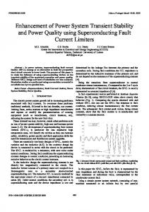
NCE contains 1614 generators, 4,791 buses and 8,206 transmission lines. The reference power is 100MVA. PMUs are deployed at 246 buses. And the EI model used in the case study is developed by the Multi-regional Modeling Working Group (MMWG) and contains approximately 29,000 buses and 4,000 generators. Most of the EI system is included in the model, but Florida and some parts of the extreme northeast have been

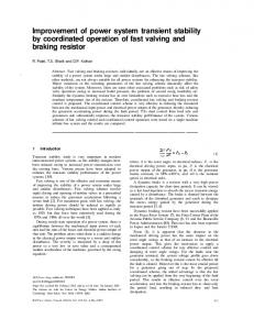
1) OC Generation: In this step, 30 operating conditions (OCs) are generated in PSD-BPA (which was developed by CEPRI and widely used in State Grid) based on the generation and load patterns provided by the system operation organization. They represent stressed OCs that include all details of load levels, generator outputs and branch power flows during a specific period of time. Some of these OCs stress the system well beyond the normal operating margins. 2) Critical Contingency Setup: A contingency list, which is created by the regional system operator to account for possible outages of transmission lines, three-winding transformers and generators that may have significant impact, is used here. Since no N-1 contingencies lead to insecure conditions, we conduct N-2 contingencies for all generators, buses and transmission lines, 24 N-3 contingencies for the pivotal sections, and 4 N-4 contingencies for each small region. 3)Offline training and testing: Perform transient security assessment by using PSD-BPA for all realized OCs and contingency, the power angle-based stability margin defined in Eq.(17) is used as the transient stability index. Thus, 50,000 samples are chosen for the procedure, 25,000 samples are used for training and the other half are used for testing. The indices for evaluating performance are shown in Table V. Fig.10 is the accuracy of SVM and CVM using PMU big data. It is easily observed that the precision of SVM and CVM both increased as the data set is scaled up. Moreover, the precision of CVM is always higher than of SVM. As the number of samples goes over to 20000, the precision stops rising.

1949-3053 (c) 2015 IEEE. Personal use is permitted, but republication/redistribution requires IEEE permission. See http://www.ieee.org/publications_standards/publications/rights/index.html for more information.

This article has been accepted for publication in a future issue of this journal, but has not been fully edited. Content may change prior to final publication. Citation information: DOI 10.1109/TSG.2016.2549063, IEEE Transactions on Smart Grid JOURNAL OF LATEX CLASS FILES, VOL. 13, NO. 9, SEPTEMBER 2014

TABLE V E VALUATION INDICES OF SVM AND CVM Samples 5000 10000 15000 20000 25000

AC SVM 93.08% 93.94% 93.62% 94.15% 94.98%

CVM 94.83% 95.07% 95.12% 95.76% 95.81%

IN BIG DATA

TT(s) SVM CVM 0.574 0.352 1.406 1.180 2.691 2.345 5.943 5.037 10.16 9.572

0.965

Num.of SV SVM CVM 462 398 1073 991 1309 1132 1923 1764 2385 2189

SVM CVM

0.96

8

Fig.11 and Fig.12 show CPU time and the number of SVs of SVM and CVM based on big data. CVM is faster and has fewer SVs than SVM which means it can handle much more data under the same condition. 4)Online TSA results and conclusions: The real PMU data of NCE are obtained with the help of CEPRI. The data is collected and managed by every 5 minutes for one year, thus 105,120 datasets in total. 10,821 faults occur within overall data, and only 734 faults may cause transient insecurity because of the strong structure and advanced operation technology of the State Grid. The offline trained CVM is applied to the 10,821 datasets, and the SVM is also used to do the assessment in comparison. And the results are shown in Table VI.

Accuracy

0.955

TABLE VI E VALUATION INDICES OF SVM AND CVM

0.95 0.945

Method SVM CVM

0.94

AC 95.10% 99.50%

FD 2.94% 0.28%

IN REAL

FA 1.96% 0.22%

NCE PMU

DATA

AT(s) 0.15 0.08

0.935 0.93 5000

10000

15000 Number of Samples

20000

25000

Fig. 10. Accuracy of SVM and CVM in big data

12

SVM CVM

10

CPU Time(s)

8

6

4

2

0 5000

10000

15000 Number of Samples

20000

B. Case Study of Eastern Interconnection In this case, the steps are similar to the NCE example. In the first step, 82 operating conditions are generated in the PSS/E EI model with the help of MMWG. The OCs represent the load patterns of EI in a standard year. Then, a contingency list including N-2,N-3 and N-4 is created. In the second step, the transient stability simulation is conducted in the PSS/E, and the dataset is built according to Section III Part A, 84,000 available samples are collected. 56,000 of them are used for training data and the remaining 28,000 samples are used for testing data. The offline test results are shown in Table VII. In the final step, the real PMU data of EI are collected and managed by every 5 minutes for one year, and 16,240 faults exist within 105,120 datasets, and only 1260 faults cause transient instability. Then the offline trained CVM and SVM are applied to 16,240 datasets, the results are shown in Table VIII.

25000

VI. C ONCLUSION Fig. 11. CPU time of SVM and CVM in big data

2500

This paper has presented an “offline training, online application” power system transient stability assessment framework based on PMU big data and the Core Vector Machine. The assessment consists of four steps. First, 24 features are selected to present the system status. Then, the CVM model is trained

SVM CVM

Number of SV

2000

1500

TABLE VII E VALUATION INDICES OF SVM AND CVM

1000

Samples 500

0 5000

10000

15000 Number of Samples

20000

Fig. 12. Number of SV of SVM and CVM in big data

25000

7000 14000 21000 28000 35000 42000 49000 56000

AC SVM 93.28% 94.12% 94.88% 95.15% 95.45% 95.80% 96.12% 96.45%

IN BIG DATA

FD CVM 96.83% 97.07% 97.12% 97.76% 97.98% 98.50% 99.10% 99.50%

SVM 4.03% 3.53% 3.07% 2.91% 2.73% 2.52% 2.33% 2.13%

FA CVM 1.74% 1.61% 1.58% 1.23% 1.11% 0.2% 0.5% 0.28%

SVM 2.69% 2.35% 2.05% 1.94% 1.2% 1.68% 1.55% 1.42%

CVM 1.43% 1.32% 1.3% 1.01% 0.91% 0.68% 0.4% 0.22%

1949-3053 (c) 2015 IEEE. Personal use is permitted, but republication/redistribution requires IEEE permission. See http://www.ieee.org/publications_standards/publications/rights/index.html for more information.

This article has been accepted for publication in a future issue of this journal, but has not been fully edited. Content may change prior to final publication. Citation information: DOI 10.1109/TSG.2016.2549063, IEEE Transactions on Smart Grid JOURNAL OF LATEX CLASS FILES, VOL. 13, NO. 9, SEPTEMBER 2014

TABLE VIII E VALUATION INDICES OF SVM AND CVM IN REAL EI PMU Method SVM CVM

AC 97.10% 99.90%

FD 1.74% 0.06%

FA 1.16% 0.05%

9

DATA

AT(s) 0.21 0.10

in an offline training procedure. Third, online TSA using the trained CVM and real time PMU big data is implemented. Finally, indices for evaluating performance are calculated. Case studies on the IEEE New England 39-bus system and real systems are used to verify the precision, time consumption and space complexity during the assessment. In addition, the best type of kernel is discussed and compared. In conclusion, results demonstrate that the highest precision, the least time consumption and the lowest space complexity of CVM algorithm may guarantee that the performance of the online TSA is the most optimal. ACKNOWLEDGMENT The authors would like to thank the National Natural Science Foundation of China (No.:51477121). R EFERENCES [1] Andersson, G.Donalek and P. Farmer, “Causes of the 2003 major grid blackouts in North America and Europe, and recommended means to improve system dynamic performance,”IEEE Trans. Power Syst., vol.20, no.4, pp.1922-1928, 2005. [2] L.Ci, Y.Sun and X.Chen, “Preliminary analysis of large scale blackout in Western Europe power grid on November 4 and measures to prevent large scale blackout in China,” IEEE Trans. Power system technology, vol. 30, no. 24, pp.16-21, 2012. [3] N.Ming, J.D.McCalley,and V.Vittal,“Software implementation of online risk-based security assessment,”IEEE Trans. Power Syst., vol.18, no.3, pp.1165-1172,2003. [4] N.Ming, J.D.McCalley,and V.Vittal, “Online risk-based security assessment,”IEEE Trans. Power Syst., vol.18, no.1, pp.258-265,2003. [5] K.Sun,S.Likhate and V.Vittal,“An Online Dynamic Security Assessment Scheme Using Phasor Measurements and Decision Trees,” IEEE Trans. Power Syst., vol.22, no.4, pp.1935-1943,2007. [6] M.L.Scala,R.Sbrizzai and F.Torelli, “A tracking time domain simulator for real-time transient stability analysis,”IEEE Trans. Power Syst., vol.13, no.3, pp.992-998, 1998. [7] N.Kakimoto,Y.Ohnogi and H.Matsuda,“Transient Stability Analysis of Large-Scale Power System by Lyapunov’s Direct Method,” Power Engineering Review, IEEE , vol.PER-4, no.1, pp.41-47, 1984. [8] V.Vittal,E.Z.Zhou, and C.Hwang,“Derivation of Stability Limits Using Analytical Sensitivity of the Transient Energy Margin,” Power Engineering Review, IEEE , vol.9, no.11, pp.33-34, 1989. [9] Y. Xue,C.T.Van Custem,and M.Ribbens-Pavella, “Extended equal area criterion justifications, generalizations, applications,” IEEE Trans. Power Syst., vol.4, no.1, pp.44-52,1989. [10] Z.Yingchen, P. Markham,and L.Yilu, “Wide-Area Frequency Monitoring Network (FNET) Architecture and Applications,” IEEE Trans.Smart Grid , vol.1, no.2, pp.159-167,2010. [11] D.L.Ree, V. Centeno,J.S.Thorp, and A.G.Phadke, “Synchronized Phasor Measurement Applications in Power Systems,” IEEE Trans.Smart Grid , vol.1, no.1, pp.20-27,2010. [12] M. Khan, L. Maozhen, P.Ashton, and L. Junyong, “Big data analytics on PMU measurements,” Fuzzy Systems and Knowledge Discovery (FSKD), 2014 11th International Conference on , pp. 715-719, December 9, 2014. [13] Jinsong Liu, Xiaolu Li, Dong Liu, Hesen Liu, Peng Mao, “Study on data management of fundamental model in control center for smart grid operation,” IEEE Trans. Smart Grid., vol. 2, pp. 573-579, Dec 2011.

[14] L. Qiao, C. Tao,W. Yang, and F.Franchetti, “An Information-Theoretic Approach to PMU Placement in Electric Power Systems,” IEEE Trans.Smart Grid, vol.4, no.1, pp.446-456,2013. [15] A. G. Bahbah and A. A. Girgis, “New method for generators’ angles and angular velocities prediction for transient stability assessment of multimachine power systems using recurrent Artificial Neural network,”IEEE Trans. Power Syst., vol. 19, pp. 1015C1022, 2004. [16] N. Amjady and S. F. Majedi, “Transient stability prediction by a hybrid intelligent system,” IEEE Trans. Power Syst., vol. 22, pp. 1275C1283,2007. [17] M. He, J. Zhang, and V. Vittal, “Robust online dynamic security assessment using adaptive ensemble decision-tree learning,” IEEE Trans. Power Syst., vol. 28, pp. 4089C4098, 2013. [18] Geeganage, J. Annakkage, U.D. Weekes, T. Archer, B.A. “ Application of Energy-Based Power System Features for Dynamic Security Assessment,” IEEE Trans. Power Syst., vol.30, no.4, pp.1957-1965,2015. [19] I .W. Tsang, A. Kocsor,J.T.Kwok, “Diversified SVM ensembles for large data set,” Machine Learning: ECML 2006, pp.792-800, 2006. [20] I. W. Tsang , J. T. Kwok , and P. M. Cheung, “Core vector machines: Fast SVM training on very large data sets,” IEEE Trans. Journal of Machine Learning Research, vol.6, pp.363-392, 2005. [21] I. W. Tsang,A. Kocsor , and J.T. Kwok, “Simpler core vector machines with enclosing balls,” Proceedings of the 24th international conference on Machine learning. ACM, pp.911-918, 2007. [22] M. Mohammadi, and G.B. Gharehpetian, “On-line transient stability assessment of large-scale power systems by using ball vector machines,” Energy Conversion and Management, vol.51, pp.640-647, 2010. [23] R. Zivanovic , and C. Cairns, “Implementation of PMU technology in state estimation: an overview,” IEEE AFRICON 4th, pp.1006-1011, 1996. [24] P. Ju , and F. Dai , WAMS for Systems, Beijing, China Machine Press, 2008. [25] H. Huang , N. Shu, and Z. Li Z, “Power system transient stability assessment based on information fusion technology,” IEEE Trans. Proceedings of CSEE, vol. 27, no. 16, pp.19-23, 2007. [26] S. Ye , X. Wang , and Z. Liu, “Dual-stage feature selection for transient stability assessment based on Support Vector Machine,” IEEE Trans. Proceedings of CSEE, vol. 30, no. 31, pp.28-34, 2010. [27] S. K. Tso , X. P. Gu , and Q. Y. Zeng Q Y, “An ANN-based multilevel classification approach using decomposed input space for transient stability assessment,” Electric Power Systems Research, vol. 46, no. 3, pp.259-266, 1998. [28] Zhao, Qingsheng, Jingyuan Dong, Tao Xia, and Yilu Liu . “Detection of the start of frequency excursions in wide-area measurements,” Power and Energy Society General Meeting-Conversion and Delivery of Electrical Energy in the 21st Century, 2008 IEEE, IEEE, 2008. [29] T.P. Ning , M. Steinbach, and V. Kumar, Introduction to data mining, Pearson Education, 2007 [30] I. Steinwart, and A. Christmann, Support Vector Machines, Springer, 2008. [31] M. Pai, Energy Function Analysis for Power System Stability, Springer, 2008.ser.Kluwer Int. Series Eng. Comput. Sci.. Berlin, Germany: Springer,1989. [32] “TSAT (Transient Security Assessment Tool) Manual”, Powertech Labs Inc., 2004. [33] “User Manual-Transient Security Assessment Tool (TSAT)”,Powertech Labs Inc., Apr. 2009.

Bo Wang (M’13) received the Ph.D. degree in computer science from Wuhan University, Wuhan, China, in 2006. And he did the postdoctoral research in the School of Electrical Engineering Wuhan university from 2007 to 2009. Dr. Wang is currently an associate professor with the School of Electrical Engineering, Wuhan University, Wuhan, China. His research interests include power system online assessment, big data, integrated energy system (IES) and smart city.

1949-3053 (c) 2015 IEEE. Personal use is permitted, but republication/redistribution requires IEEE permission. See http://www.ieee.org/publications_standards/publications/rights/index.html for more information.

This article has been accepted for publication in a future issue of this journal, but has not been fully edited. Content may change prior to final publication. Citation information: DOI 10.1109/TSG.2016.2549063, IEEE Transactions on Smart Grid JOURNAL OF LATEX CLASS FILES, VOL. 13, NO. 9, SEPTEMBER 2014

Biwu Fang received the B.S. degree in School of Electrical Engineering Wuhan University, Wuhan, Hubei, China, in 2014, where he is currently persuing the M.S degree of power system and automation. His research interests include power system transient stability analysis, robust dispatch of renewable energy system and the application of data mining technology in power system.

Yajun Wang received the B.S. and M.S. degrees in School of Electrical Engineering Wuhan University, Wuhan, Hubei, China, in 2012 and 2014, respectively. She is currently pursuing the Ph.D. degree in electrical engineering in the Department of Electrical Engineering and Computer Science, University of Tennessee, Knoxville, TN, USA. She is also a graduate research assistant with the department of Electrical Engineering and Computer Science, the University of Tennessee, Knoxville, US. Her research interests include power system stability and control, energy storage system and data mining.

10

Hesen Liu (S16) received the B.S. degree in electrical engineering from North China Electric Power University, Beijing, China, in 2005. He is currently pursuing the Ph.D. degree in electrical engineering in the Department of Electrical Engineering and Computer Science, University of Tennessee, Knoxville, TN, USA. He was at Yunnan Power Grid Company, Kunming, China, from 2005 to 2011. His current research interests include wide-area power system measurement, power system dynamics and control.

Yilu Liu (M’89-SM’99-F’04) received her M.S. and Ph.D. degrees from the Ohio State University, Columbus, in 1986 and 1989, respectively. She received the B.S. degree from Xian Jiaotong University, China. Dr. Liu is currently the UT-ORNL Governor’s Chair at the University of Tennessee, Knoxville and Oak Ridge National Laboratory (ORNL). She is also the deputy Director of the DOE/NSF engineering research center CURENT. Prior to joining UTK/ORNL, she was a Professor at Virginia Tech. She led the effort to create the North American power grid Frequency Monitoring Network (FNET) at Virginia Tech, which is now operated at UTK and ORNL as GridEye. Her current research interests include power system wide-area monitoring and control, large interconnection-level dynamic simulations, electromagnetic transient analysis, and power transformer modeling and diagnosis.

1949-3053 (c) 2015 IEEE. Personal use is permitted, but republication/redistribution requires IEEE permission. See http://www.ieee.org/publications_standards/publications/rights/index.html for more information.