Powered Addition as Modelling Technique for Flow ... - CiteSeerX

Powered Addition as Modelling Technique for Flow Processes by

Pierré de Wet Thesis presented in partial fulfilment of the requirements for the degree of Master of Sciences at Stellenbosch University

Supervisor: Prof. J P du Plessis

Department of Mathematical Sciences Applied Mathematics Division Faculty of Natural Sciences March 2010

http://scholar.sun.ac.za

Declaration By submitting this thesis electronically, I declare that the entirety of the work contained therein is my own, original work, that I am the owner of the copyright thereof (unless to the extent explicitly otherwise stated) and that I have not previously in its entirety or in part submitted it for obtaining any qualification.

Signature: . . . . . . . . . . . . . . . . . . . . . . . . . . .

Date: . . . . . . /. . . . . . /. . . . . . . . . . . .

i


Abstract The interpretation – and compilation of predictive equations to represent the general trend – of collected data is aided immensely by its graphical representation. Whilst, by and large, predictive equations are more accurate and convenient for use in applications than graphs, the latter is often preferable since it visually illustrates deviations in the data, thereby giving an indication of reliability and the range of validity of the equation. Combination of these two tools – a graph for demonstration and an equation for use – is desirable to ensure optimal understanding. Often, however, the functional dependencies of the dependent variable are only known for large and small values of the independent variable; solutions for intermediate quantities being obscure for various reasons (e.g. narrow band within which the transition from one regime to the other occurs, inadequate knowledge of the physics in this area, etc.). The limiting solutions may be regarded as asymptotic and the powered addition to a power, s, of such asymptotes, f 0 and f ∞ , leads to a single correlating equation that is applicable over the entire domain of the dependent variable. This procedure circumvents the introduction of ad hoc curve fitting measures for the different regions and subsequent, unwanted jumps in piecewise fitted correlative equations for the dependent variable(s). Approaches to successfully implement the technique for different combinations of asymptotic conditions are discussed. The aforementioned method of powered addition is applied to experimental data and the semblances and discrepancies with literature and analytical models are discussed; the underlying motivation being the aspiration towards establishing a sound modelling framework for analytical and computational predictive measures. The purported procedure is revealed to be highly useful in the summarising and interpretation of experimental data in an elegant and simplistic manner.

ii


Opsomming Die interpretasie – en samestelling van vergelykings om die algemene tendens voor te stel – van versamelde data word onoorsienbaar bygestaan deur die grafiese voorstelling daarvan. Ten spyte daarvan dat vergelykings meer akkuraat en geskik is vir die gebruik in toepassings as grafieke, is laasgenoemde dikwels verskieslik aangesien dit afwykings in die data visueel illustreer en sodoende ’n aanduiding van die betroubaarheid en omvang van geldigheid van die vergelyking bied. ’n Kombinasie van hierdie twee instrumente – ’n grafiek vir demonstrasie en ’n vergelyking vir aanwending – is wenslik om optimale begrip te verseker. Die funksionele afhanklikheid van die afhanklike veranderlike is egter dikwels slegs bekend vir groot en klein waardes van die onafhanklike veranderlike; die oplossings by intermediêre hoeveelhede onduidelik as gevolg van verskeie redes (waaronder, bv. ’n smal band van waardes waarbinne die oorgang tussen prosesse plaasvind, onvoldoende kennis van die fisika in hierdie area, ens.). Beperkende oplossings / vergelykings kan as asimptote beskou word en magsaddisie tot ’n mag, s, van sodanige asimptote, f 0 en f ∞ , lei tot ’n enkel, saamgestelde oplossing wat toepaslik is oor die algehele domein van die onafhanklike veranderlike. Dié prosedure voorkom die instelling van ad hoc passingstegnieke vir die verskillende gebiede en die gevolglike ongewensde spronge in stuksgewyspassende vergelykings van die afhankilke veranderlike(s). Na aanleiding van die moontlike kombinasies van asimptotiese toestande word verskillende benaderings vir die suksesvolle toepassing van hierdie tegniek bespreek. Die bogemelde metode van magsaddisie word toegepas op eksperimentele data en die ooreenkomste en verskille met literatuur en analitiese modelle bespreek; die onderliggend motivering ’n strewe na die daarstelling van ’n modellerings-raamwerk vir analitiese- en rekenaarvoorspellingsmaatreëls. Die voorgestelde prosedure word aangetoon om, op ’n elegante en eenvoudige wyse, hoogs bruikbaar te wees vir die lesing en interpretasie van eksperimentele data.

iii


Acknowledgements I would like to express my sincere gratitude to the following people for their contribution: • My supervisor, Prof. Jean Prieur du Plessis, for patient academic guidance, longanimity and an open-door policy throughout the course of both my undergraduate and postgraduate studies at Stellenbosch University; • Prof. Britt Halvorsen at Høgskolen i Telemark (Telemark University College), Porsgrunn, Norway, for being my host and generous financial assistance during my visit to their institution during the months of August – October 2008; for encouraging me to write a paper for submission to The 5th International Conference on Computational & Experimental Methods in Multiphase and Complex Flow (Multiphase Flow V); and for making it financially possible to attend the conference in New Forest, UK, form 15 - 17 June 2009; • Dr. Finn Haugen for writing the experiment-specific software in L AB V IEW that we required to perform the experiments at Høgskolen i Telemark (Telemark University College), Porsgrunn, Norway. • The South African National Research Foundation (NRF) for financial support.

iv


vir die Twee Outes

v


Contents

Declaration

i

Abstract

ii

Acknowledgements

iv

Dedication

v

Nomenclature

ix

Introduction

xiii

1 Powered addition as curve fitting technique

1

1.1

Asymptotic behaviour of transfer processes . . . . . . . . . . . . . . . . .

1

1.2

Shifting of the matching curve . . . . . . . . . . . . . . . . . . . . . . . . .

4

1.2.1

Increasing dependence . . . . . . . . . . . . . . . . . . . . . . . . .

4

1.2.2

Decreasing dependence . . . . . . . . . . . . . . . . . . . . . . . .

6

1.2.2.1

Bounded from below . . . . . . . . . . . . . . . . . . . .

6

1.2.2.2

Bounded from above . . . . . . . . . . . . . . . . . . . .

7

1.2.3

Only limiting values known . . . . . . . . . . . . . . . . . . . . . .

9

1.2.4

Crossing of one limiting solution . . . . . . . . . . . . . . . . . . . 15

vi


CONTENTS

vii

1.3

Normalisation to obtain one horizontal asymptote . . . . . . . . . . . . . 17

1.4

Critical point and shifting-exponent . . . . . . . . . . . . . . . . . . . . . 18

2 Flow in straight-through diaphragm valves

21

2.1

Definitions of pressures and heads . . . . . . . . . . . . . . . . . . . . . . 22

2.2

Choice of Reynolds number . . . . . . . . . . . . . . . . . . . . . . . . . . 25

2.3

Mbiya’s empirical correlation . . . . . . . . . . . . . . . . . . . . . . . . . 26

2.4

Powered addition applied to Mbiya’s work . . . . . . . . . . . . . . . . . 28

3 Flow through a packed bed

34

3.1

Ergun equation . . . . . . . . . . . . . . . . . . . . . . . . . . . . . . . . . 35

3.2

RUC model . . . . . . . . . . . . . . . . . . . . . . . . . . . . . . . . . . . 38 3.2.1

Granular porous media . . . . . . . . . . . . . . . . . . . . . . . . 39

3.2.2

Spongelike porous media . . . . . . . . . . . . . . . . . . . . . . . 40

3.2.3

Unidirectional two-dimensional fibre-bed porous media . . . . . 42

4 Fluidised bed 4.1

44

Newtonian fluid . . . . . . . . . . . . . . . . . . . . . . . . . . . . . . . . . 45 4.1.1

4.1.2

4.1.3

Experimental procedure . . . . . . . . . . . . . . . . . . . . . . . . 45 4.1.1.1

Superficial velocity of the traversing fluid . . . . . . . . 47

4.1.1.2

Porosity of the packed bed . . . . . . . . . . . . . . . . . 47

Asymptotic dependencies . . . . . . . . . . . . . . . . . . . . . . . 49 4.1.2.1

The lower asymptote . . . . . . . . . . . . . . . . . . . . 49

4.1.2.2

The upper asymptote . . . . . . . . . . . . . . . . . . . . 51

Powered addition of the asymptotes . . . . . . . . . . . . . . . . . 52 4.1.3.1

Critical point and shifting-exponent . . . . . . . . . . . . 52


CONTENTS

viii 4.1.3.2

4.1.4 4.2

Crossing of the upper asymptote . . . . . . . . . . . . . 53

Correlation of experimental results . . . . . . . . . . . . . . . . . . 54

Non-Newtonian fluid . . . . . . . . . . . . . . . . . . . . . . . . . . . . . . 58 4.2.1

4.2.2

Asymptotic dependencies . . . . . . . . . . . . . . . . . . . . . . . 58 4.2.1.1

The lower asymptote . . . . . . . . . . . . . . . . . . . . 58

4.2.1.2

The upper asymptote . . . . . . . . . . . . . . . . . . . . 60

Powered addition of the asymptotes . . . . . . . . . . . . . . . . . 60 4.2.2.1

4.2.3

Critical point and shifting-exponent . . . . . . . . . . . . 61

Correlation of experimental results . . . . . . . . . . . . . . . . . . 62

5 Conclusion / Closure

64

A Fluid classification

66

A.1 Newtonian flow . . . . . . . . . . . . . . . . . . . . . . . . . . . . . . . . . 66 A.2 Non-Newtonian flow . . . . . . . . . . . . . . . . . . . . . . . . . . . . . . 68 B Derivation of Slatter Reynolds number

70

C Plots with Mbiya’s data sets

77

D Høgskolen i Telemark (Telemark University College) data sets

98


Nomenclature Constants π e

3.141 592 654 2.718 281 828

Variables av A Aann Ac Ap Aplug Asp B c cd CΩ d dp ds dsv dv D Dh Dplug D Dshear f {x}

particle specific surface arbitrary coefficient area of annulus cross-sectional area of bed surface area of single, non-spherical particle area of plug surface area of an equivalent volume sphere arbitrary coefficient constant form drag coefficient new constant / model parameter of Mbiya linear dimension of RUC mean particle diameter linear dimension of solid in RUC diameter of sphere with equivalent surface area / volume ratio as particle volume diameter diameter hydraulic diameter plug diameter diameter of sphere (perfectly spherical particle) sheared diameter original dependent variable ix

[m−1 ] [− ] [m2 ] [m2 ] [m2 ] [m2 ] [m2 ] [− ] [− ] [− ] [− ] [m] [m] [m] [m] [m] [m] [m] [m] [m] [m] [− ]


x f0 f∞ g g{ x } h{ x ∗ } hv hs ht H k kv kv, c K L m0 mf ms M n N p pH q qA qm f Qann Qplug r rplug R Re Re3 Re3, c Re p Re s t U0 Uf Us v

asymptotic solution or correlation for x → 0 asymptotic solution or correlation for x → ∞ acceleration due to gravity canonical dependent variable logarithmic dependent variable velocity head static head total head bed height pressure loss coefficient pressure loss coefficient for valve pressure loss coefficient for valve at critical point fluid consistency index length of straight channel / bed height total or bulk mass mass of traversing fluid solid mass empirically determined, constant coefficient fluid behaviour index empirically determined, constant coefficient pressure total pressure head superficial velocity / specific discharge arbitrary constant minimum fluidisation velocity flux through annulus flux through plug radius plug radius pipe radius general Reynolds number Slatter Reynolds number Slatter Reynolds number at critical point particle Reynolds number Reynolds number for packed bed of spheres arbitrary shifting exponent arbitrary shifting exponent total or bulk volume volume of fluid phase volume of solid phase velocity

[− ] [− ] [m/s2 ] [− ] [− ] [m] [m] [m] [m] [− ] [− ] [− ] [Pa.sn ] [m] [kg] [kg] [kg] [− ] [− ] [− ] [N/m2 ] [N/m2 ] [m/s] [− ] [m/s] [m3 /s] [m3 /s] [m] [m] [m] [− ] [− ] [− ] [− ] [− ] [− ] [− ] [m3 ] [m3 ] [m3 ] [m/s]


xi vann vplug vx vy vz Vp w x x∗ xA xB xc Y z Z

corrected mean velocity in the annulus velocity of plug velocity component in x-direction velocity component in y-direction velocity component in z-direction volume of single, non-spherical particle specific weight independent variable logarithmic independent variable arbitrary constant arbitrary constant independent variable at central or critical point normalised dependent variable height above arbitrary reference point normalised independent variable

[m/s] [m/s] [m/s] [m/s] [m/s] [m3 ] [kg/m2 s2 ] [− ] [− ] [− ] [− ] [−] [− ] [m] [− ]

Greek letters α β γ˙ ∆ ε ε0 η θ κ λΩ µ ν ζ 0 {q} ζ ∞ {q} ρ ρ0 ρf ρs τ τ0

exponent in asymptotic solution for x → 0 / arbitrary exponent exponent in asymptotic solution for x → ∞ / arbitrary exponent shear rate change in stream-wise property bed porosity / void fraction porosity at incipient fluidisation apparent viscosity valve opening coefficient hydrodynamic permeability nominal turbulent loss coefficient fluid dynamic viscosity kinematic viscosity functional dependence of pressure drop for q → 0 functional dependence of pressure drop for q → ∞ mass density total or bulk mass density mass density of traversing fluid mass density of solids shear stress shear stress at the pipe wall

[− ] [− ] [s−1 ] [− ] [− ] [− ] [N.s/m2 ] [− ] [− ] [− ] [N.s/m2 ] [s−1 ] [N/m3 ] [N/m3 ] [kg/m3 ] [kg/m3 ] [kg/m3 ] [kg/m3 ] [N/m2 ] [N/m2 ]


xii τy φp Φ ψ Ψ

yield stress particle shape factor (sphericity) variable defined for simplicity in Ergun equation geometric factor Waddell sphericity factor

[N/m2 ] [− ] [−] [− ] [− ]

Vectors and Tensors f b nˆ ∇ σ τ

body forces unit vector in stream-wise direction del operator stress tensor viscous stress dyadic

Acronyms CHE RUC

Churchill-Usagi Equation Representative Unit Cell

[N/kg] [− ] [m−1 ] [N/m2 ] [N/m2 ]


Introduction The dependence of modern engineering research on precise, credible experimental and computational practices is undeniable. These procedures provide the requisite predictive information needed for design purposes and the in-depth understanding of complex processes. It is common practice to represent the general trend in a set of such collected data by drawing a line through the individual datum points on the plot. Correlation between the drawn predictive curve and the data is then evaluated against some norm, e.g. least squares fit to a straight line or polynomial function passing through the data, visual inspection, etc. Theoretical knowledge of the functional behaviour is helpful but not a prerequisite for the construction of graphical correlation and thus a line best suited to the particular problem is chosen – the better the predictive line on the graphical presentation corresponds to the physical reality, especially in the limits of the independent variable, the greater the trustworthiness of obtained results. If it is possible to accurately determine or predict the asymptotic behaviour – traits at extreme values of the independent variable – of the dependent variable under consideration, the results can usually be presented in a neat and elegant format. The basic procedure of asymptotic matching by straightforward addition of the expressions for the asymptotic conditions is a method that has been been in use for some time, especially in engineering practice. However, the article by Churchill & Usagi [1], which appeared in 1972, for the first time really formalised the use and accentuated the wide application possibilities of the method and variations thereof. Their method yields an equation of simple form with one arbitrary constant that interpolates between the limiting solutions; the value of which may be determined by either experimental or theoretical procedure. The routine is applicable to any phenomenon which varies uniformly between known, limiting solutions and is especially useful for the evaluation and summarising of experimental and computational data. Furthermore it is particularly convenient for design purposes as it yields an expression that is relevant over the entire domain of the dependent variable and has the same form for all correlations. Whether it presents an exact representation of the transfer process cannot be proven scientifically, yet the method is widely applicable and accepted.

xiii


xiv In the first chapter an outline is given of powered addition. The articles by Churchill & Usagi [1; 2] form the backbone of this chapter. Different scenarios of the limiting functions and / or values are investigated and simple examples provided. Curve adjustment and the importance of the point of intersection of the asymptotes are discussed. Chapter 2 and 4 sees the application of the method to the collected experimental data for two diverse processes. The results of the former chapter were presented at The 2nd Southern African Conference on Rheology (SASOR), Cape Peninsula University of Technology, Cape Town, 6 - 8 October 2008 [3]; those of the latter were published in the proceedings of The 5th International Conference on Computational & Experimental Methods in Multiphase and Complex Flow (Multiphase Flow V), New Forest, UK, 15 - 17 June 2009 [4]. Chapter 3 serves as précis of two approaches used in predicting pressure drop over a packed bed or porous medium – the one (Ergun equation) being itself an example of powered addition with an exponent of unity, the other (RUC model) forming a keystone to the work of the following chapter. Supplementary material and the original data sets of the experimental investigations conducted at Høgskolen i Telemark (Telemark University College), Porsgrunn, Norway are collected in the appendices.


Chapter 1 Powered addition as curve fitting technique Powered addition of expressions valid for two opposing ranges as described by Churchill and Usagi [1; 2; 5; 6] is a procedure used to produce a combined result which is valid for both of these ranges. Since each of the limiting expressions predominates in their respective regions of applicability, a unified model can be obtained using such an ‘asymptote matching’ technique.

1.1 Asymptotic behaviour of transfer processes In many continuum processes, such as momentum and thermal transfer processes, the value of a sought after parameter is expressible as a function of certain known parameter(s) at low and high values. These limiting solutions for large and small values of the independent variable(s) may be regarded as asymptotic conditions of the dependent variable. By stating that f { x } → g{ x } it is meant that

f {x} g{ x }

as

x→a

→ 1 as x → a.

In other words, it is said that f is asymptotic to g as x → a [7]. Very often the functional expression of the dependent variable is in the form of a power dependency upon some independent variable, x.

1


1.1 Asymptotic behaviour of transfer processes

2

Let the functional dependence, f , of such a process be described by f → f 0 { x } = Ax α

as

f → f ∞ { x } = Bx β

as

x → 0,

(1.1)

x → ∞.

(1.2)

Here equations (1.1) and (1.2) denote the functional expressions at the lower and upper extremal values of x respectively. However, solutions for intermediate cases are seldom as simply expressed. (It is important to take note that, for the discussion to follow, the explicit expression of the asymptotes in terms of a power dependency is not permutable, i.e. the lower asymptote is always associated with coefficient A and exponent α; the upper with B and β). The direct summation of two such asymptotic solutions or approximations is often effected to obtain a single solution that holds over the entire range of the independent variable, i.e. (1.3) f { x } = f 0 { x } + f ∞ { x } = Ax α + Bx β . Equation (1.3) may now be considered as a matching or coupled curve connecting the two dependencies as it satisfies the asymptotic conditions and also provides values for f at intermediate values of the independent variable, x.

3.5

3

2.5

f {x}

2

1.5

1 f0 = 1 0.5

f∞ = x f {x} = f0 + f∞

0

0

0.5

1

1.5

2

2.5

3

x

Figure 1.1: Linear plot of the function f { x } = 1 + x.

3.5


1.1 Asymptotic behaviour of transfer processes

3

As an example, consider the very simple case of a function f { x } = 1 + x; i.e. A = 1, B = 1, α = 0 and β = 1 in equation (1.3). In the above formulation this corresponds to the case, f { x } → 1 as

f {x} → x

as

x → 0,

(1.4)

x → ∞.

(1.5)

Hence the asymptotes governing the behaviour of the coupled function will be given by f0 {x} = 1

f ∞ { x } = x. Plotting this relation on a linear-linear Cartesian scale, generates a straight line as shown in Figure 1.1. It is only once the function is drawn on a log-log graph that more insight is gained; the asymptotic behaviour that results from addition of the functional expressions at the extremal values now becomes apparent. This is illustrated in Figure 1.2. 2

10

1

f {x}

10

0

10

f0 = 1 f =x ∞

f {x} = f0 + f∞ −1

10

−2

10

−1

10

0

10 x

1

10

2

10

Figure 1.2: Log-log plot of the function f { x } = 1 + x. The advantage of using logarithmic coordinates when plotting data is that equal percentage changes yield equal displacements over the entire range, where-as with


1.2 Shifting of the matching curve

4

arithmetic coordinates (Cartesian axes) on the other hand, the displacement increases in accordance with the magnitude of the variable. In other words, logarithmic coordinates display percentage deviations and perceptually suppress these deviations compared to arithmetic plots – the former may thus obscure the magnitude of scatter in the data, the latter distort such scatter unduly by displaying absolute differences. [5]. It is important to note that, as seen in Figure 1.1, the matched curve merely approaches, yet never reaches, the upper limiting functional value. An increase in the independent variable leads to the diminishing influence of the lower asymptotic function on the overall solution, which only becomes visually apparent once the solution is plotted on log-log axes as in Figure 1.2. The method is therefore best suited to approximate the general trend in a process, rather than predict the exact values of the constituent limiting functions.

1.2 Shifting of the matching curve Frequently the values of the dependent variable at the transition between the asymptotic extremities do not lie exactly on this matching solution. Churchill & Usagi [1; 2; 5; 6] demonstrated that the use of powered addition, the most general form of which is shown in equations (1.6) and (1.7) below, may lead to dramatic improvement in correlation with experimental data s { x }, f s { x } = f 0s { x } + f ∞

(1.6)

s f { x } = [ f 0s { x } + f ∞ { x }]1/s .

(1.7)

whence

By adjusting the value of the shifting exponent, s, the level of the solution may be modified so as to more closely trace the expected or empirical values, yielding better correspondence between predictive equation and experimental results. The right hand side of equation (1.7) may be considered as the sth order sum of the asymptotic solutions [1; 2; 5].

1.2.1 Increasing dependence When the dependent variable is an increasing power of the independent variable, in other words if the power of x in equation (1.3) is greater at the higher limit, that is α < β,

(1.8)



5

2.5

f {x}

2

1.5

f0

1

s=1 s=2 s=5

f∞ 0.5

0

0.5

1

1.5

2

x

s { x }]1/s = [1 + x s ]1/s for Figure 1.3: Linear plot of the function f { x } = [ f 0s { x } + f ∞ varying values of the shifting exponent, s.

the expression f { x } = [( Ax α )s + ( Bx β )s ]1/s ,

(1.9)

is usually desirable for interpolation between the extremal values. Theoretically the matched function in equation (1.9) will have no upper bound and will only be bounded from below by the the functional expression for small values of x; i.e the term Ax α in equation (1.3) will form a lower bound on the values that the independent variable may take on. The arbitrary exponent, s will now have a positive value. The shifting effect obtained is illustrated in Figures 1.3 and 1.4; the same conditions were used as in equations (1.4) and (1.5) to obtain s f { x } = [ f 0s { x } + f ∞ { x }]1/s = [1 + x s ]1/s .

(1.10)

For the sake of simplicity, the function-notation ( f 0 and f ∞ ) will henceforth be favoured over the explicit expression in terms of power dependencies.


6

f {x}


f0

0

10

f∞

s=1 s=2 s=5 −2

10

−1

0

10

10 x

s { x }]1/s = [1 + x s ]1/s for Figure 1.4: Log-log plot of the function f { x } = [ f 0s { x } + f ∞ varying values of the shifting exponent, s.

1.2.2 Decreasing dependence In some instances the dependence of f { x } decreases with an increase in the independent variable, i.e. α > β, (1.11) in equation (1.3). Two possibilities now exist – the asymptotes may either form the lower bound or the upper bound of the resulting matched curve; knowledge of the process being modelled and/or experimental data will dictate the specific case.

1.2.2.1 Bounded from below Decreasing dependence upon the independent variable is such that the solutions for extremal values – i.e. the functional expressions for the asymptotes – bind all possible solutions to the process from below. Suppose, for the sake of an illustrative example,



7

3 s=1 s=2 s=5 2.5

f {x}

2

1.5

f 1

∞

f0 0.5

0.5

1

1.5

2

2.5

3

x

Figure 1.5: Linear plot of the function f { x } = shifting exponent, s.

h s 1 x

+1

i1/s

for varying values of the

that the limiting solutions to such a process are given by the simple relations 1 as x f { x } → 1 as

f {x} →

x → 0,

(1.12)

x → ∞.

(1.13)

This corresponds to equation (1.3) with coefficients A = 1, B = 1 and exponents, α = −1 and β = 0. The matched solution, raised to the shifting exponent will thus be 1/s s 1 +1 . f {x} = x

(1.14)

The result of varying the values of the shifter, s, is graphically represented on Cartesian and log-log axes in Figures 1.5 and 1.6 respectively.

1.2.2.2 Bounded from above The asymptotes, f 0 { x } and f ∞ { x }, of the process being modelled form an upper bound on the possible values that the function can assume. Using the formulation of



8

1

f {x}

10

f∞

0

10

f0

s=1 s=2 s=5 −1

10

0

1

10

10 x

Figure 1.6: Log-log plot of the function f { x } = the shifting exponent, s.

h s 1 x

+1

i1/s

for varying values of

equation (1.3) consider, as an example, the very simple case in which the asymptotes constituting the matched equation are given by f {x} → x

as

f { x } → 1 as

x → 0,

x → ∞.

(1.15) (1.16)

To ensure that the matched solution approaches the limiting functions from below, the shifting exponent now needs to take on a negative value. However, the obtained curve will still approach the asymptotes as |s| increases; illustrated in Figures 1.7 and 1.8. The introduction of a negative value for s may be circumvented by taking the reciprocal of the original dependent variable, i.e. by defining 1 1 1 1 1 + = = + , g{ x } Ax p Bx q g0 { x } g ∞ { x }

(1.17)

before it is raised to s, ensures that s > 0. Applying this to the above example, outlined in equations (1.15) and (1.16), yields the function f {x} =

x , 1+x

(1.18)



9

1.5

f0 f

∞

f {x}

1

0.5

s = −1 s = −2 s = −5 0

0

1

2

3 x

4

5

6

Figure 1.7: Linear plot of the function f { x } = [ x s + 1]1/s for varying negative values of the shifting exponent, s. and in so doing Figures 1.7 and 1.8 in g{ x } are converted to Figures 1.5 and 1.6 in f { x } = 1/g{ x }.

1.2.3 Only limiting values known In many cases the functional dependence of the independent variable is known at the extremal values. Often, however, only the limiting values in both limits, i.e. f {0} and f {∞}, are known beforehand. In cases such as these the straight-forward application of equation (1.6) is not possible and an alternative approach is to be followed. To commence, a functional dependence of the dependent variable upon the independent variable is postulated for either x → 0 or x → ∞. Any convenient function which approximates the behaviour of the data may be chosen. Churchill & Usagi [2] recommend the use of a power function since its use is widely applicable and the simplicity of such a function ties in with that of equation (1.6) and the philosophy behind the method in general. Once an applicable function for either of the limiting values has been chosen it is, as per the discussion in Section 1.1, matched to the constant value



10

f {x}

f0

f

∞

0

10

s = −1 s = −2 s = −5

−1

10

−1

0

10

1

10

2

10

10

x

Figure 1.8: Log-log plot of the function f { x } = [ x s + 1]1/s for varying negative values of the shifting exponent, s. that binds the process in the other limit (it is important to choose the approximating function such that no singularities are introduced once the functions are combined). As an example, the power function f 0 { x } = f {0} + ( f {∞} − f {0})

x xA

α

,

(1.19)

may be suggested to represent the functional dependence at the lower limiting value [2]. Here x A is an arbitrary constant and α an arbitrary exponent; the influence of these values on the obtained curves will be discussed shortly. The function in equation (1.19) is chosen such that f 0 { x } → f {0} i.e.

( f {∞} − f {0})

x xA

α

→0

as

x → 0,

as

x → 0.

(1.20)

In equation (1.20) the coefficient ( f {∞} − f {0}) is a constant value and therefore it should hold that α x (1.21) → 0 as x → 0, xA



11

f{∞}

1

f0{x}

10

x =1 f{0}

0

10

A

xA = 2 xA = 5

−2

10

−1

0

10

1

10

10

x

Figure 1.9: Postulated function f 0 { x } = f {0} + ( f {∞} − f {0})( x/x A )α for constant value of arbitrary exponent, α = 1.5, and varying values of the arbitrary constant, x A . which will only be the case if both the arbitrary constant and exponent is such that x A > 0 and α ≥ 0; a restriction that should be kept in mind when choosing these values. The postulated function and upper limiting asymptote will now intersect where f 0 { x } = f ∞ { x }, that is f {0} + ( f {∞} − f {0})

x xA

whence, after rearrangement and division, α x = 1. xA

(1.22) α

= f { ∞ },

(1.23)

(1.24)

It thus follows from equation (1.24) that x = x A at the intersection of these two functions; by changing the value of x A the point of intersection may be altered. In Section 1.4 the importance of this value, the so-called critical point, will be discussed. Plotting of the postulated function in equation (1.19) for different values of the arbitrary constant x A – illustrated in Figure 1.9 – graphically clarifies its influence.



12

f{∞}

1

f0{x}

10

α=1 α=2 α=5

f{0}

0

10

−2

10

−1

0

10

10

1

10

x

Figure 1.10: Postulated function f 0 { x } = f {0} + ( f {∞} − f {0})( x/x A )α for constant value of the arbitrary constant, x A = 1, and varying values of the arbitrary exponent, α. The influence of the arbitrary exponent, α, becomes clear when equation (1.19) is rearranged as α f { x } − f {0} x , (1.25) = 0 xA f { ∞ } − f {0} and the logarithm taken on either side to yield α x f 0 { x } − f {0} log = log , xA f { ∞ } − f {0} i.e.

α(log x − log x A ) = log( f 0 { x } − f {0}) − log( f {∞} − f {0}).

(1.26)

Defining a new variable, x ∗ , equation (1.26) thus takes the form of a linear depen-



13

f0{x} f{∞}

1

f{x} = 1/g{x}

10

f{0}

0

10

−2

10

−1

s=1 s=2 s=5

0

10

1

10

10

x

Figure 1.11: Application of powered addition with only limiting values known. A function of the form f 0 { x } = f {0} + ( f {∞} − f {0})( x/x A )α was postulated for the lower limiting dependency. The effect of varying the value of the shifting exponent, s, on the solution is shown (x A = 1 and α = 2 were kept constant). dency in x ∗ (straight line graph in Cartesian coordinates), such that

where

h{ x ∗ } = αx ∗ + c,

(1.27)

h{ x ∗ } = log( f 0 { x } − f {0}),

(1.28)

x ∗ = log x,

(1.29)

and c is a constant value c = log( f {∞} − f {0}) − α log x A = log

f { ∞ } − f {0} x αA

.

(1.30)

As can be seen from equation (1.27), altering the value of α thus influences the ’curvature’ of the postulated function; this is illustrated graphically in Figure 1.10. The postulated function of equation (1.19) will thus form an upper bound on the possible values that the dependent variable may take in the lower limit. Furthermore



14

s=1 s=2 s=5 f{∞}

1

f{x} = 1/g{x}

10

f {x} 0

f{0}

0

10

−2

−1

10

0

10

1

10

10

x

Figure 1.12: Application of powered addition with only limiting values known. A function of the form f ∞ { x } = f {∞} − ( f {∞} − f {0})( x B /x ) β was postulated for the upper limit. The effect on the matched solution for selected values of the shifting exponent, s, is demonstrated (x B = 1 and β = 1.5 were kept constant). its contribution to the final solution should diminish as the value of the independent variable increases, in other words, once matched, the solution should show a decreasing dependence upon this function: a decreasing dependence, bounded from above as outlined in Section 1.2.2. By setting g{ x } = 1/ f { x }, cf. equation (1.17), the expressions g0 { x } = 1/ f 0 { x } and g∞ { x } = 1/ f ∞ { x } = 1/ f {∞} are obtained for the respective dependencies; the latter being a constant value. Inserting the aforementioned together with the proposed dependency of equation (1.19) into equation (1.6), yields 1 f s {x}

=

1 f 0s { x }

+

1 s {x} f∞

=

1

x f {0} + ( f {∞} − f {0}) xA

α s +

1 f s {∞}

.

(1.31)

A plot of equation (1.31) for different values of the shifting exponent, s, is shown in Figure 1.11. Instead of postulating a function for the lower limit, the behaviour of the process in



15

the upper limit may be considered. The function is now required to act such that f ∞ { x } → f {∞}

as

x → ∞.

(1.32)

Once again a power function, now of the form f ∞ { x } = f {∞} − ( f {∞} − f {0})

x β B

x

,

(1.33)

may be utilised as arbitrary function, approximating the dependency at upper extremal values. Applying the same reasoning as above to equation (1.32) imposes the restrictions x B > 0 and β ≥ 0 (the function now forming a lower bound). A power-added function, similar to that of equation (1.31), covering the entire range of the independent variable, may now be constructed by choosing g{ x } = 1/ f { x }, g0 { x } = 1/ f 0 { x } = 1/ f {0} and g∞ { x } = 1/ f ∞ { x }, where 1/ f 0 { x } is now given by equation (1.33). Figure 1.12 illustrates the use of the function proposed in equation (1.33) for approximation of the behaviour at upper extremal values; altering the value of the shifting exponent, s, having the desired effect.

1.2.4 Crossing of one limiting solution In some phenomena the data is not bound completely by the limiting solutions; one of the limiting functions may be crossed as the solution approaches it. Although it is presumed that both the lower functional dependency, f 0 { x }, and the upper limiting value, f {∞}, is known, equation (1.6) is not directly applicable, since for any positive values of the shifting exponent, equation (1.6) gives values that fall above f 0 { x } and f {∞} (see Sections 1.2.1 and 1.2.2.1). As in the preceding section, a function is postulated viz., f ∞ { x } → f {∞} as x → ∞, (1.34) but it should now differ from equation (1.33) in that it not only forms an upper bound on attainable values of the dependent variable, but also approaches the limiting value from above. Using a function of the form [1; 2], h x α i A , (1.35) f ∞ { x } = f {∞} 1 + x

in stead of f {∞}, solves this problem, since as x → ∞ the second term in square brackets on the left hand side of equation (1.35) approaches zero (once again, provided that α ≥ 0).

Constructing a new dependency of the form suggested by equation (1.6), with g{ x } = 1/ f { x }, g0 { x } = 1/ f 0 { x } and g∞ { x } = 1/ f ∞ { x }, with f ∞ { x } the newly defined re-



16

f∞{x}

1

f{x} = 1/g{x}

10

s=1 s=2 s=5

f{0}

0

10

f{∞}

0

1

10

2

10

10

x

Figure 1.13: Application of powered addition when the solution crosses one of the limiting functions; a function of the form f ∞ { x } = [1 + ( x A /x )α ] utilized to approximate the upper limit. The effect on the matched solution for selected values of the shifting exponent, s, is demonstrated (x A = 5 and α = 2 were kept constant). lation of equation (1.35), yields

f0 {x} f {x}

s



 = 1+

s

f0 {x}  h x α i  A f {∞} 1 + x

(1.36)

after simplification. In Figure 1.13 the family of curves found for selected values of the shifting exponent, s is illustrated; the arbitrary variables, x A = 5 and α = 2, were kept constant, their allocated values having been selected purely for demonstrative purposes. Investigation of the influence of the arbitrary constant, x A , and arbitrary exponent, α, in equation (1.36) can be done in a fashion similar to the procedures followed to obtain equations (1.26) and (1.27) – the graphical representation of a change in the values assigned to these constants are illustrated by Figures 1.14 and 1.15. The results are, as was to be expected, akin to those of Figures 1.9 and 1.10.


1.3 Normalisation to obtain one horizontal asymptote

f∞{x}

1

10

17

xA = 1

f{0}

xA = 2 x =5

f{x} = 1/g{x}

A

0

10

f{∞}

0

1

10

2

10

10

x

Figure 1.14: Variation of the value of the arbitrary constant, x A , in equation (1.35) with the value of arbitrary exponent, α = 2, being kept constant.

1.3 Normalisation to obtain one horizontal asymptote Frequently neither of the expressions for the limiting solutions, (1.1) and (1.2), are linear in form or of a constant value. To aide visual interpretation it is often beneficial to divide equation (1.7) by one of the asymptotic expressions, namely s 1/s f {x} f ∞ {x} = 1+ , f0 {x} f0 {x} or f {x} = f ∞ {x}

f0 {x} f ∞ {x}

s

+1

1/s

,

(1.37)

(1.38)

to obtain non-dimensional, normalised forms of the original function. Both equation (1.37) and (1.38) can now be written in generic form as Y = (1 + Zs )1/s ,

(1.39)

yielding a horizontal asymptote at Y = 1 (Z → 0); the exact functional definition of the newly defined variables, Y and Z, will be case specific. Plotting of the expression


1.4 Critical point and shifting-exponent

18

f∞{x}

1

α=1 α=2 α=5

f{x} = 1/g{x}

10

f{0}

0

10

f{∞}

0

1

10

10

2

10

x

Figure 1.15: The effect of a change in the arbitrary arbitrary exponent, α, on the asymptotes of the Churchill-Usagi equation proposed by equation (1.35). The value of the arbitrary constant, x A = 5, was kept constant. obtained in equation (1.37) will stretch the curve at low values of the independent variable, whereas plots with equation (1.38) will extend the curve at high values of the independent variable.

1.4 Critical point and shifting-exponent The central or critical point, xc , of the matching curve is the value of the independent variable at which the asymptotes meet. Since the asymptotes intersect here, the numerical value of their respective functional expressions must be equal, that is f 0 { x c } = f ∞ { x c }.

(1.40)

As both functions, f 0 and f ∞ , contribute equally to the added solution at this point, the resultant curve is most sensitive to variations in the value of the shifter, s, in the vicinity of xc . Furthermore, looking at equations (1.37), (1.38) and (1.39), it becomes apparent that the maximal fractional deviation of the matched solution from either of



19

3.5

3

2.5 ( xc, f {xc} )

f {x}

2

1.5

1 f0 = 1 0.5

f∞ = x f {x} = f0 + f∞

0

0

0.5

1

1.5

2

2.5

3

3.5

x

s { x })1/s = (1 + x s )1/s to Figure 1.16: Linear plot of the function f { x } = ( f 0s { x } + f ∞ indicate the location of the critical point and equivalent function value.

the limiting solutions or asymptotic values will occur at precisely this point and take on the value (1.41) Y {1} − 1 = 21/s − 1. That is

f { xc } f 0 { xc }

−1 =

f { xc } f ∞ { xc }

− 1 = 21/s − 1,

(1.42)

if written in terms of the original equations for the extremal values. Determining the value of the shifting-exponent, s, we use the same argument as above in equation (1.40). Thus, s s f s { xc } = f 0s { xc } + f ∞ { xc } = 2 f 0s { xc } = 2 f ∞ { xc }

(1.43)

whence it follows that

f { xc } f ∞ { xc }

s

=

f { xc } f 0 { xc }

s

= Y {1}s = 2.

(1.44)

The value of s may now be determined straightforwardly from equation (1.44) as s=

ln 2 ln 2 ln 2 = = . ln f { xc } − ln f ∞ { xc } ln f { xc } − ln f 0 { xc } ln Y {1}

(1.45)



20

2

10

1

f {x}

10

( x , f {x } ) c

c

0

10

f0 = 1 f∞ = x f {x} = f0 + f∞ −1

10

−2

10

−1

10

0

10 x

1

10

2

10

s { x })1/s = (1 + x s )1/s to Figure 1.17: Log-log plot of the function f { x } = ( f 0s { x } + f ∞ indicate the location of the critical point and equivalent function value.

In performing an experiment, it is therefore advantageous to arrange the physical conditions in such a manner that the independent variable is in close vicinity of xc . Whenever the experimental value of f { xc } is known, we proceed to determine the value of the shifter by equation (1.45). In Figures 1.16 and 1.17 the critical point and the corresponding function value at this point is indicated for the illustrative example, f { x } = 1 + x, that has been used thus far. Note that in this, most simple form, the value of the shifter, s = 1. Alternatively, visual inspection by trial and error adjustment of the correlation between the predictive curve and data points may lead to an assignment of a value to s. As noted by Churchill & Usagi [1] the matched curve is relatively insensitive to variations in s; the required acuity being determined by considerations such as the process involved, tunability of other parameters and allowable error-margin.


Chapter 2 Flow in straight-through diaphragm valves Diaphragm valves possess several advantages that lead to their extensive use in diverse industrial applications. There are two types of diaphragm valves: the "weir" type used in piping systems that carry less viscous fluids; and the "straight-through" type - a schematic representation of which is shown in Figure 2.1 - suited to slurries and suspensions [8]. The data sets of Mbiya [9; 10], on which this chapter is based, is concerned with the latter type of valve.

Figure 2.1: Schematic representation showing the cross-section of a straight-through diaphragm valve (http://www.engvalves.com) Despite the broad scope of their use, Mbiya [9; 11] notes that few studies dealing 21


2.1 Definitions of pressures and heads

22

with valve openings of aperture less than unity is available in the literature. This limits the use of the information contained therein, rendering it inapplicable to cases where valves are used as flow impeding devices. Furthermore the studies that had been done were restricted to specific intervals of the Reynolds number. The aim of Mbiya’s [9; 11] experimental investigation was to more accurately predict the additional pressure loss incurred, for four different opening positions, once a pipe had been fitted with a straight-through diaphragm valve. A brief outline will be given on the definition of the pressure loss coefficient, the experimental determination of which is one of the main focuses of Mbiya’s work [9; 10; 11]. Hereafter the specific Reynolds number used in his study will be discussed shortly (for a complete derivation of the Slatter Reynolds number, refer to Appendix B). In the second half of this chapter Mbiya’s [9; 11] results are investigated for possible asymptotic bounds whereafter powered addition is applied to these functional dependencies. The outcomes of powered addition is compared to those of Mbiya’s model for a few selected cases (a complete set of comparative graphs are available in Appendix C) and the results discussed.

2.1 Definitions of pressures and heads The fitting of a valve into a pipe section causes a change in shape of the plane perpendicular to the direction of flow and hence also in that of the flow path, thereby leading to an increase in the pressure drop as the fluid traverses the constriction caused by the valve. In Figure 2.2 this resulting additional pressure loss is graphically illustrated. A wide variety of parameters are used to express the pressure drop characteristics of the different components in a piping system [12]. The data on pressure losses may be arrived at by either experiment or by theoretical solution of the equations governing flow. Pressure loss data obtained by the former method usually concern measurements taken at two stations, one upstream and one downstream of the component. Reference is seldom made to the details of the change in pressure within the component itself. The well-known Bernoulli equation for steady, incompressible flow states 1 p 1 2 p1 v1 + + gz1 = v22 + 2 + gz2 = constant, 2 ρ1 2 ρ2

(2.1)

where v is the velocity, p the pressure, ρ the fluid density (which is presumed constant), z is the height above some arbitrary reference point and g is the acceleration due to gravity. Division of equation (2.1) by g yields v21 v2 p p + 1 + z1 = 2 + 2 + z2 = constant = ht , 2g w1 2g w2

(2.2)


23

Pressure, p


∆p, pressure drop over valve

additional pressure drop due to valve

valve position

Pipe length

Figure 2.2: Increased pressure drop due to the presence of a valve. where w, the specific weight, has been written in stead of ρg. The terms in equation (2.2) all have the dimensions of length and are referred to as heads in hydraulics. Hence, v2 /2g is known as the velocity head (hv ), p/w the pressure head, z is the position head and their sum, ht – constant along the stream tube – is called the total head [12]. Frequently the pressure head and position head together are referred to as the static head [13]; the choice of this grouping becomes clear upon regarding Figure 2.3, where the flow in a horizontal pipe is schematically represented. The height to which a fluid rises in a tube connected to a tapping in the pipe wall is called the static head. The difference between the static head and the head yielded upon placing a forward facing tube (pitot) into the fluid stream, is called the velocity head. The total head is simply the sum of the static and velocity heads. Comparison with equation (2.2) yields an expression for the static head hs =

p + z. w

(2.3)

Since it is the same fluid being regarded, and assuming incompressibility (i.e. constant density), that is ρ = ρ1 = ρ2 , equation (2.1) may be multiplied by ρ, resulting in 1 1 2 (2.4) ρv1 + p + ρgz1 = ρv22 + p + ρgz2 = constant = p H . 2 2 In equation (2.4) the contribution to the energy balance (the principle on which the



24

velocity head, v2 2g

total head, v2 hs + 2g static head, hs

Figure 2.3: Graphical representation of the static, velocity and total heads. Bernoulli equation is based) of the term ρgz is negligible [12] and hence it simplifies to 1 2 1 ρv1 + p1 = ρv22 + p2 = constant = p H . 2 2

(2.5)

In the form of equation (2.5) all terms have the dimensions of pressure; the first term, 1 2 2 ρv , is known as the dynamic pressure, the second term, p, as the static pressure and their sum, p H , (once again a constant along the stream tube) as the total pressure [12]. Considering equation (2.5), it follows that any change in the total or static pressure within the flow will be proportional to the local dynamic pressure. This leads to the definition of the total pressure loss coefficient k≡

p¯ H2 − p¯ H1 1 2 2 ρv

=

∆p H . 1 2 2 ρv

(2.6)

Hence, using the change of total head, the head loss, ∆ht , in a straight pipe section is approximately proportional to the square of the velocity, v2 , of the fluid. The relation in equation (2.6) may thus be expressed as k=

h t1 − h t2 2g∆ht 2gH = = 2 , 2 2 v¯ /2g v¯ v¯

(2.7)

whereby division of the head loss by the mean velocity head, v¯2 /2g, yields a nondimensional loss coefficient [12; 13]. The presence of a component, such as a valve, in a piping system will, via an increase in the loss of dynamic pressure, lead to a


2.2 Choice of Reynolds number

25

larger head loss. The study of Mbiya [9; 10; 11] concerns the experimental determination of the pressure loss coefficient (or resistance coefficient) and the prediction thereof in terms of an empirical equation expressible as a function of valve opening and Reynolds number.

2.2 Choice of Reynolds number According to Newton’s law of viscosity the shear stress, τ, and viscosity, µ, for onedimensional flow of a fluid are related by τ = −µ

dv x , dy

(2.8)

where dv x /dy is the shear rate or velocity gradient as a function of position [14]. Fluids that obey this criterion are referred to as Newtonian fluids. This is however an idealisation as many fluids exhibit a more complicated relationship than the mere linearity described by equation (2.8). Often the relation between the velocity gradient and shear stress of a fluid is best described by the power dependency, dv x n τ=K − , (2.9) dy where K is the fluid consistency index and n the flow behaviour index; fluids exhibiting such behaviour are called power-law fluids (for a brief outline on the classification of fluids, refer to Appendix A). Depending on the value of the flow behaviour index, power-law fluids are classified into three broad groups: pseudo-plastic fluids if n < 1; Newtonian fluids for n = 1, since equation (2.9) reverts to equation (2.8) in this case; and dilatant fluids for n > 1. In pseudo-plastic substances shear thinning is observed, in other words the viscosity decreases with an increase in rate of the shear stress. A true plastic substance has an initial yield stress that needs to be overcome before it assumes fluid-like properties, i.e. continuous deformation when subjected to a (further) shear stress [14]. The constitutive equation for the yield pseudo-plastic model can thus be formulated as dv x n τ = τy + K − , (2.10) dy

with τy denoting the yield stress. Setting n = 1 in equation (2.10) yields the so-called Bingham-plastic model, while τy = 0 results in it reverting back to that for power-law fluids, equation (2.9).

The Slatter Reynolds number, Re3 , is based on the yield pseudo-plastic model and starts from the assumption that, in the presence of a yield stress, the core of the fluid


2.3 Mbiya’s empirical correlation

26

moves as a solid, unsheared plug [10; 15] resulting in annular flow (see derivation in Appendix B). It can be expressed as Re3 =

8ρv2ann 8vann n τy + K Dshear

.

(2.11)

In equation (2.11) vann denotes the corrected mean velocity in the annulus and Dshear the sheared diameter.

2.3 Mbiya’s empirical correlation The addition of a component, such as a valve, to a piping system leads to a local constriction (or dilation) of the cross-sectional area and consequently also to a change in the flow path. Initially, at low Reynolds numbers – the region of laminar flow –

Re → 0

0 < Re < 10

Re → ∞ Figure 2.4: Schematic representation of recirculation within the valve section due to an increase in the Reynolds number. streamlines will trace out the irregular geometry caused by the valve’s presence. As the Reynolds number increases however, localised areas of recirculation will gradually develop within the indentations of the diaphragm until, at turbulent flow conditions,


2.3 Mbiya’s empirical correlation

27

the streamlines bypass these areas altogether; Figure 2.4 represents this schematically. This is an intuitive explanation accounting for the constant resistance coefficients (pressure loss) obtained at high Reynolds numbers, i.e. turbulent flow, and reflected in the data of Mbiya [9; 10; 11]. Mbiya’s [9; 10; 11] proposed two-constant model is based on a large set of accrued experimental data. A test rig , constructed at the Cape Peninsula University of Technology, consisted of pipes of different diameters (40mm, 50mm, 65mm, 80mm and 100mm), each of which was fitted with the appropriately sized diagram valve. The fluids carboxymethyl cellulose [CMC] (at 5% and 8% concentration), glycerine or glycerol (concentrations of 75% and 100%), kaolin, a claylike mineral (10% and 13% concentrations) and water were pumped through the pipes for four different valve opening positions (25%, 50%, 75% and 100% open) and the pressure drop in the pipe was recorded. The aim was to predict the pressure loss coefficient, kv ( Re3 ), as defined in equation (2.7) – the v-subscript denoting valve – for straight-through diaphragm valves. Mbiya [9; 10; 11] concludes by summarizing his model, as being applicable to all sizes of valves tested, by straight-forward addition of  1000   , Re3 < 10    Re3 kv = (2.12)   λ C  Ω  + Ω , Re3 ≥ 10  √ 2 θ2 Re3 θ Here CΩ is a new constant (model parameter) introduced by Mbiya [9; 11], λΩ is the nominal turbulent loss coefficient, and θ is the partial valve opening coefficient as ratio of the fully opened position, i.e. θ = 0 for a closed valve and θ = 1 for a fully opened valve. Note that an open valve does not correspond to an open tube flow condition; the diaphragm still protrudes into the lumen as can be seen in Figure 2.1 (right).

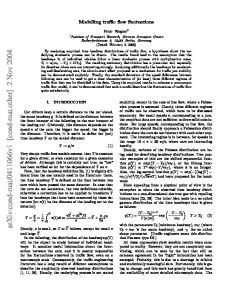
Unfortunately, to obtain good agreement with experimental results, an ‘if’-condition had to be introduced at a Slatter Reynolds number of 10. The two different curve fitted solutions on either side of this value lead to an unwanted jump in the values of the dependent variable, i.e. the predicted crossover at this Reynolds number is not smooth; Figure 2.5 shows a typical correlation for such a case – cf equation (2.12) – the ‘jump’ in the value of the dependent variable evident. This contradicts the expected, intuitive-orderly behaviour of such a continuum transfer process. (The constant CΩ is an unfortunate fudge factor introduced for proper agreement, in the transitional region, between the experimental data and correlative equations (2.12). It is also this factor that leads to the unwanted jump in the proposed model).


2.4 Powered addition applied to Mbiya’s work

28

CMC 5% CMC 8% Glycerine 100% Kaolin 10%

2

kvθ2 / λΩ

10

1

10

0

10

2

4

10

10

6

10

Re3λΩ / θ2

Figure 2.5: Typical correlation of experimental data with equation (2.12), showing the jump at Re3 = 10. The equations were applied to the data sets of Mbiya [9] for a pipe with internal diameter of 40mm and a valve opening of 25%.

2.4 Powered addition applied to Mbiya’s work Regarding equation (2.12) in the limit where Re3 → ∞, it is clear that kv → λΩ /θ 2 . Hence, λΩ /θ 2 may be regarded as an asymptotic lower bound on kv . The direct addition of this result to the dependency of kv on Re3 for Re3 < 10, is then considered as a matching between the two asymptotic conditions, yielding a single solution that covers the entire range of the Reynolds numbers, namely kv =

1000 λΩ + 2. Re3 θ

(2.13)

Inspection of Mbiya’s proposal thus evidently leads to the following definitions k0 ≡

1000 Re3

k∞ ≡

λΩ θ2

and

for

for

Re3 → 0,

(2.14)

Re3 → ∞,

(2.15)



29

whence equation (2.13) becomes k v = k0 + k ∞ .


2

10

kvθ2 / λΩ

(2.16)

1

10

0

10

2

4

10

10

6

10

Re3λΩ / θ2

Figure 2.6: Application of powered addition to the data sets generated by Mbiya [9] for a pipe with internal diameter of 40mm and a valve opening of 25%; s-values of 0.4 (solid line) and 1.4 (dashed) are shown for comparison.

Instead of the direct addition of the two asymptotes as in equation (2.13), powered addition, as discussed in Chapter 1, may now be applied to the asymptotic expressions, yielding ksv = ks0 + ks∞ , (2.17) which may, analogous to equation (1.38), be re-written as s 1/s kv k0 = +1 . k∞ k∞

(2.18)

If two new variables, Y and Z, are defined as kv k∞ k0 Z≡ , k∞ Y≡

(2.19) (2.20)



30

equation (2.18) simplifies to Y = [ Zs + 1]1/s ,

(2.21)

cf equation (1.39). Instead of dividing equation (2.17) by k∞ , one may alternatively have chosen to designate k0 as denominator, followed by the corresponding redefinition of variables Y and Z in equations (2.19) and (2.20). One extremely useful consequence of this type of modelling is the direct possibility of non-dimensionalisation into either of the following forms (1/s) kv Re3 λΩ Re3 s = 1+ , (2.22) 1000 1000 θ 2 or " #(1/s) s kv θ 2 1000 θ 2 (2.23) = +1 . λΩ λΩ Re3 Furthermore, in so doing equations (2.22) and (2.23) have been normalized with regards to different values of the nominal turbulent loss coefficient, λΩ , and valve flow ratio (or valve opening), θ, and a single horizontal asymptote obtained. Determination of the critical point and the value of the shifting exponent may now be done in the manner outlined in Section 1.4. The critical point will thus be where k0 = k ∞ ,

(2.24)

whence λ 1000 = Ω Re3, c θ2 1000 θ 2 ⇒ Re3, c = . λΩ

(2.25)

Since both λΩ and θ are constants for a given pipe diameter and valve opening, the Slatter Reynolds number at which the critical point is to be found may easily be determined; these values are listed in Table 2.1. The pressure loss coefficient at the critical point is thus given by kv,c = kv ( Re3, c ), the corresponding functional value obtained by equation (2.25). The discussion in Section 1.4, equation (1.45), now yields a value for the shifting exponent, i.e. ln 2 ln 2 s= = , (2.26) ln kv, c − ln k∞, c ln kv, c − ln k0, c or in explicit form as s=

ln 2 ln kv ( Re3, c ) − ln

λΩ θ2

=

ln 2 ln kv ( Re3, c ) − ln

1000 Re3, c

.

(2.27)



31

valve opening, θ

40mm 50mm 65mm 80mm 100mm

(λΩ (λΩ (λΩ (λΩ (λΩ

= 8.0) = 3.4) = 1.5) = 2.9) = 4.1)

0.25

0.50

0.75

1.00

7.8594 18.493 41.917 21.681 15.335

31.438 73.971 167.67 86.724 61.341

70.734 166.43 377.25 195.13 138.02

125.75 295.88 670.67 346.90 245.37

Table 2.1: Calculated values Re3, c = (1000 θ 2 )/λΩ for all possible combinations of pipe diameter and valve opening. The λΩ -values in this table were obtained from Mbiya [9]. Traversal of the data sets in search of the Re3, c -value closest to those listed in Table 2.1 may now be effected, the objective being to find the corresponding value of the dependent variable, kv, c , at this point. Plugging these values into equation (2.27) will then yield a possible value for the shifting exponent. However, the datum point chosen may be a poor choice (an outlier, the result of a poor reading, etc.) and grounding the s-value solely on this one, single reading may lead to erroneous results. It is therefore recommended that the value of the intersection of the asymptotes be determined beforehand and the bulk of experimentation conducted in the area of the yielded independent variable, i.e. Re3, c . In so doing a more accurate prediction will be obtained (from averaging numerous data points) and the fractional deviation of the matched solution from either of the limiting solutions or asymptotic values minimized (see Section 1.4). It is nevertheless important to note that the method is still an empirical one, based on experimental results; the wish being for an analytical expression in which this shifting exponent is linked to some quantifiable parameter in the process under consideration. Since Mbiya’s experimental readings were not arranged in such a manner as to focus on the transitional area between the asymptotes, the aforementioned methodical approach was not used. In lieu, to circumvent the shifting exponent being based on an incorrect or inaccurate reading, a trial-and-error graphical approach was used. The results of two such curve fittings for different pipe diameters and valve openings are shown in Figures 2.6 and 2.7, with s-values of 0.4 (solid line) and 1.4 (dashed) plotted for comparison. Ideally, the normalised, non-dimensional expressions of equations (2.22) and (2.23) would also allow for the experimental data of all valve sizes to be plotted on a single plot, irrespective of the valve flow ratio, θ. However, as can be seen in Table 2.1, there is no discernable relation between the valve diameter and the λΩ -values. Mbiya



32

CMC 5% CMC 8% Glycerine 100% Kaolin 10% H2O

2

kvθ2 / λΩ

10

1

10

0

10

2

10

4

10

6

10

Re3λΩ / θ2

Figure 2.7: Powered addition applied to Mbiya’s [9] data sets for a pipe with internal diameter of 50mm and a valve opening of 50%. s-values of 0.4 (solid line) and 1.4 (dashed) are shown for comparison. [9; 10; 11] notes that λΩ is obtained by the minimisation of the overall logarithmic difference between his calculated and experimental kv -values and cites the lack of dynamic similarity between valves of different sizes as rationalisation for these discrepancies. An attempt at plotting all the data for a specific valve diameter, regardless of the valve opening, on a single plot afforded no clear visual results. To prevent clutter, data sets were plotted on separate axes according to valve diameter and valve opening (see Appendix C). The plots show a gradual shift towards and beyond (below) the asymptotes with an increase in the valve opening, that is to lower values of both the dependent and independent variables. This observation suggests a dependence upon some parameter that is yet to be considered or identified. To arrive at an accurate prediction of the shifter it is recommended that experiments be tailored so as to specifically investigate the flow parameters in the transitional regime; this was, however, not the focus of Mbiya’s [9; 11] study. Although the graphs obtained through the use of powered addition still leave a lot



33

to be desired, overall they exhibit, for our particular goal, a qualitatively improved prediction of the process than the model of Mbiya.


Chapter 3 Flow through a packed bed Packed beds are of significant interest to chemical engineers since they are widely used for mass transfer in industrial plants. A crucial piece of information required for effective design is the difference of piezometric head necessary to ensure steady fluid flow, be it through a pipe, porous medium, etc. See e.g. [16] (piezo is derived from the Greek piezein, which means to squeeze or press). In the study of porous media this translates into a relation being sought between the pressure gradient and the superficial or discharge velocity. The two predominant approaches used in the theoretical study of pressure drop through a packed bed differ from one-another in the manner in which the solid and fluid parts of the bed are regarded. The first method regards the pores between the solid phase as a bundle of tangled tubes of irregular and inconsistent cross-section and proceeds to develop a model based on applying, modifying and expanding the wellestablished results for the flow in single, straight tube. The second method involves the solid phase being seen as an aggregation of individual objects submersed in the fluid phase; the pressure drop being calculated by addition of the resistance of each of the particles, e.g. [17]. The former approximation to reality has enjoyed more publicity and attention in the literature. In this chapter two methods used in predicting pressure drop over a packed bed or porous medium are discussed: the first, the Ergun equation, is semi-empirical in nature and, surprisingly, one of the very few known example of powered addition with an exponent of unity; the other method, the RUC model, is an analytical approach based on pore-scale modelling of the microstructure of the porous medium and forms a key concept in the discussion following in Chapter 4.

34


3.1 Ergun equation

35

3.1 Ergun equation One of the pioneers in experimental fluid mechanics was the French engineer, Henry Darcy (1803 - 1858) of Dijon. Involvement in the design of municipal water supply systems led to his research into the flow of water through sand bed filters [18; 19] (i.e. flow through porous media) and the eventual publication in 1856 of Les Fontaines Publiques de la Ville de Dijon. The empirical law that he proposed, and that consequently carries his name, states that the rate of flow through a bed of packed particles is proportional to the pressure drop (hydraulic gradient) over the bed [18; 20] – specific discharge is proportional to the fluid pressure gradient in the direction of flow. In one dimension this linear relation is expressed as

−

dp µ = q, dx κ

(3.1)

where −dp/dx is the streamwise pressure drop, µ the viscosity of the traversing fluid and q the superficial velocity or specific discharge. The coefficient of proportionality, κ, is referred to as the hydrodynamic permeability and is generally determined experimentally (a great deal of work has gone into determining an analytical expression and will be discussed in Section 3.2). In practice, however, results obtained from experiments tend to deviate from the linear relation predicted by equation (3.1) and become nonlinear at higher velocities, despite the fact that the Reynolds number, Re, may still be fairly small [17]. Hence, wide application of Darcy’s law is impeded by its limitation to a fairly narrow range of Reynolds numbers. Throughout history various attempts have been made to more accurately relate the pressure gradient and superficial velocity. In 1901 Forchheimer proposed [21] (referenced in [22]) the introduction of a quadratic term to take this nonlinear behaviour into account, leading to an empirical generalized form of the Darcy equation, namely

−

dp = Mq + Nq2 , dx

(3.2)

with the coefficients M and N empirical constants that depend on the structural and geometric properties of the porous medium and fluid viscosity [23; 24]. In the case of a superficial velocity, q, less than unity the second term in equation (3.2) becomes negligible and it effectively reduces to the Darcy law, equation (3.1). Conversely, for a high superficial velocity the quadratic term in equation (3.2) predominates. Between these two flow regimes a transitional area exists. The Ergun equation – a capillary tube model widely used for the prediction of pressure drop of flow through a packed bed – is in essence based upon a combination of


3.1 Ergun equation

36

specific asymptotic solutions for the Darcy and Forchheimer regimes and is therefore semi-empirical in nature. In it’s derivation the assumption is made that the bed consists of smooth, uniformly sized, spherical particles; that the particles are packed in a statistically uniform random manner; and, that the diameter of the containing column is orders of magnitude larger than that of the particles. Ergun simply added the equation proposed by Blake and Kozeny for laminar flow (Darcy regime) Φ = 150Re ,

(3.3)

to the Burke-Plummer equation for turbulent flow (Forchheimer regime) [1; 17; 25], Φ = 1.75Re2 ,

(3.4)

Φ = 150Re + 1.75Re2 ,

(3.5)

to obtain an expression for the pressure drop across a packed bed for Reynolds numbers rang2

10

1

Φ / 150 Res

10

0

10

Carman−Kozeny eqn. Burke−Plummer eqn. Ergun eqn.

−1

10

−2

10

−1

10

0

10 Res / 85.7

1

10

2

10

Figure 3.1: Logarithmic correlation for the pressure drop through a packed bed of spheres – the Ergun equation is an instance of powered addition with s = 1 (the equation of Carman and Kozeny was added to the Burke-Plummer equation). ing from the laminar to the turbulent flow regimes. It should be noted that the nonlinear effects, represented by the second term on the righthand side of equation (3.5),


3.1 Ergun equation

37

are already noticeable at Reynolds numbers well below that of the region which is normally associated with turbulence. His result mostly yields satisfactory agreement with experimental data for ε < 0.5. In equations (3.3) to (3.5) the variable Φ has been used for simplicity and is defined as ρ f ε3 D 3 Φ= 2 µ (1 − ε )3

dp − dL

,

(3.6)

with the Reynolds number for a packed bed of spheres, Re , given by [1] Re =

ρ f qD . µ (1 − ε )

(3.7)

In equations (3.6) and (3.7), ρ f denotes the density of the traversing fluid, ε the bed porosity or void fraction, D the diameter of a perfectly spherical particle and L the length of the straight channel (or height of bed). Ergun had thus, in effect, applied the matching technique proposed by Churchill & Usagi [1; 2; 5; 6; 25] as discussed in Chapter 1 to produce a combined result, Φ = [(150Re )s + (1.75Re2 )s ]1/s ,

(3.8)

with equation (3.8) reverting to equation (3.5) by choosing the shifting exponent, s = 1; his result is shown in Figure 3.1. The value of the exponent was however not known a priori. Utilizing the generic form suggested by equation (1.39) with Y=

Φ , 150Re

(3.9)

and

Re 1.75Re = , (3.10) 150 85.7 the value of the critical point, as considered in Section 1.4, is obtained at Z = 1, that is at Re = 85.7. Churchill [1] notes that this process happens to be the only one thus far examined in which the best choice of exponent turned out to be unity. Z=

The Ergun equation, expressed in its more well-known form

−

∆p (1 − ε)2 µq (1 − ε) ρq2 = 150 + 1.75 , L ε3 φ2p d2p ε3 φ p d p

(3.11)

takes into account cases in which the bed consists of non-spherical particles. In equation (3.11) d p denotes the mean particle diameter and φ p the particle shape factor (sphericity). The mean particle diameter, d p , is defined in terms of the specific surface, av of the particle, 6 dp = , (3.12) av


3.2 RUC model

38

with the specific surface being defined as av =

total particle surface . volume of the particles

(3.13)

The reason for the above definitions becomes apparent when regarding a bed consisting of N perfectly spherical particles. Since the surface area of a sphere is given by 4πr2 and its volume by 34 πr3 , substitution into equation (3.13) will yield av =

3 4Nπr2 6 = = , 3 4/3Nπr r D

(3.14)

and plugging this result into equation (3.12) sets d p = D (here r and D respectively denote the radius and diameter of the sphere) [17]. More often than not the bed does not consist of perfectly spherical particles, in which case it is customary to construct a hypothetical equivalent-volume sphere, φ p d p , with dp =

6Vp 6Vp = , A p φp Asp

(3.15)

as used in equation (3.11). Here Vp is the volume of a single, non-spherical particle, A p its surface area and Asp the surface area of an equivalent volume sphere. Equation (3.15) thus relates the surface area of the particle to the surface area of a sphere of equal volume [24]; cf equation (3.13). Thus, φ p = 1 and φs < 1 for spherical and non-spherical particles respectively. According to Geldart [26] the most appropriate parameter for use in flow through packed beds is the external surface area of the powder per unit particle volume. Hence, the diameter of a sphere with the same external surface area to volume ratio as that of the particle, dsv , is the most relevant diameter. The Waddell sphericity factor, Ψ, defined as surface area of equivalent volume sphere Ψ= , (3.16) surface area of particle can be shown to link dsv and dv , , by Ψ=

dsv , dv

(3.17)

with dv the volume diameter, i.e. the diameter of a sphere having the same volume as the particle.

3.2 RUC model The analytical approach to flow through porous media is based on modelling the microstructure of the porous media on pore-scale level and aims to provide a theoretical


3.2 RUC model

39

derivation of the empirical Ergun equation. In dealing with porous media that is assumed to have a regular pattern, the idea of constructing a repetitive unit or cell, holds the advantage that flow around each and every solid particle in the medium need not be analyzed. It would thus be possible to ‘reconstruct’ the particular porous medium under regard from such a building block or unit cell, provided that these cells are both volume-conserving and space-filling. The actual interstitial pore space, especially in cases where the media under regard is isotropic, and the solid material is thus randomly positioned within the volume, is very seldom open to precise analysis. To circumvent this obstacle, a hypothetical representative unit cell (RUC) was introduced [27; 28] which theoretically approximates the porous material in that it contains the average geometric properties of the material. The RUC model is thus a generalised geometric approximation of the actual geometric properties of the medium in such a manner as to preserve the physical attributes of flow through such a medium; an abstraction of the porous medium rendering it amenable to physical analysis. The pore-scale geometric relation between the solid and fluid phases of porous media allows for classification into three fundamental classes: granular, spongelike and unidirectional two-dimensional fibre-bed. Analytical expressions for the hydrodynamic permeability, k, and stream-wise pressure drop,−dp/dx, of the different RUCs are known [27; 28; 29; 30; 31; 32]. For the remainder of this section the particle Reynolds number, Re p – an indicator of the ratio between the inertial and viscous forces of the fluid with d p used as characteristic length – has been defined as Re p =

ρqd p , µ

(3.18)

where ρ and µ denote the density and viscosity of the traversing fluid respectively, q the magnitude of the superficial velocity or specific discharge and d the linear RUC dimension. The practical use of the Reynolds number is to distinguish among flow regimes, for example laminar or turbulent flow in pipes or around immersed objects, its value depending upon the situation.

3.2.1 Granular porous media In media that fall into this class, the solid phase is present in the form of isolated to semi-connected units that are submerged in the surrounding fluid phase. Some examples of granular porous media would be the glass spheres used in packed bed chemical reactors and a pipe filled with sand or marbles. A schematic representation


3.2 RUC model

40

Uo

Uf nˆ

d ds Us

Figure 3.2: Cubic geometry of the RUC model for modelling fluid flow through granuˆ The shaded volume represents lar media. The streamwise direction is indicated by n. the solid phase. of the isotropic granular RUC model [29; 31; 32] is shown in Figure 3.2. Us denotes the volume of the solid phase, U f the volume of the fluid phase and Uo the total volume of the RUC. The relation between the linear dimensions d and ds of the granular RUC, with ε denoting the porosity, is given by ds = (1 − ε)1/3 d,

(3.19)

and the stream-wise pressure drop, −dp/dx, by

−

dp c d (1 − ε ) 25.4(1 − ε)4/3 µq ρq2 = · + · , dx (1 − (1 − ε)1/3 )(1 − (1 − ε)2/3 )2 d2s 2ε(1 − (1 − ε)2/3 )2 ds

(3.20)

where cd denotes the drag coefficient and Re is the Reynolds number as defined in equation (3.18).

3.2.2 Spongelike porous media Spongelike or consolidated porous media are distinguished from granular porous media by the fact that the solid and fluid phases are interconnected. In other words, one would be able to move from any point in a given phase to any other point in the same phase, without ever having to leave it. Examples would be plastic and metallic foams, such as those used in electronics, or any substance containing interlinking ducts.


3.2 RUC model

41

Foamlike media is further differentiated into three sub-models depending on the number of stagnant pore-sections assumed to be present within the foam model [29; 33; 34]. For porous media of this type, the stream-wise pressure drop, −dp/dx is given by 36ψ2 (ψ − 1) µq cd (ψ − 1)ψ2 (ψ − 3)2 ρq2 dp = , (3.21) − · 2 + · dx ε2 d 4ε3 d with ψ a geometric factor, defined in this case as 4π 1 −1 ψ = 2 + 2 cos (3.22) + cos (2ε − 1) , 3 3 subject to the condition that ψ = 1 when ε = 1. nˆ Uo

Us

d

Uf nˆ d − ds

ds

Figure 3.3: Cubic geometry of the RUC model for modelling fluid flow through foamˆ Note that here the shaded like media. The streamwise direction is indicated by n. volume is representative of the fluid phase. In Figure 3.3 a schematic representation is given of the isotropic foamlike RUC model. It is important to note that in this figure, as opposed to the other figures, the shaded volume is representative of the fluid phase, U f . Fluid traversing such a theoretically constructed medium would thus enter through the façade facing the reader, move along the side of the cube and then turn Eastwards to move along the middle channel. It will travel a distance ds along the side of the cube, before turning in a Northerly direction, to finally exit the model at the backward facing plane. Expressing the relation between the linear dimensions d and ds of the foamlike RUC in terms of the porosity, ε, yields a polynomial of the third order, 2 3 ds ds ε = 1−3 +2 , (3.23) d d


3.2 RUC model

42

which may be rewritten in terms of the geometric factor, ψ, as [29] 4 ψ = . ε (3 − ψ )2

(3.24)

3.2.3 Unidirectional two-dimensional fibre-bed porous media Should the solid phase of the medium consist of aligned, disjoint fibre strands surrounded by an interconnected fluid phase, it is classified as a two-dimensional prismatic or unidirectional fibre-bed porous medium. Air flowing through a stack in a timber-drying kiln would be an example of porous media of this kind. Figure 3.4 shows a schematic representation of porous media of this type. It should be noted that the dimension L should be of sufficient length so as to clearly distinguish it from the granular RUC model illustrated in Figure 3.2. The relation between d and ds for the

nˆ Uo ds Uf

d

Us

L

Figure 3.4: RUC model for modelling fluid flow through fibre beds. The streamwise ˆ The shaded volume represents the solid phase. direction is indicated by n. fibre-bed RUC may be expressed as

√ ds = d 1 − ε,

(3.25)

while the stream-wise pressure drop, −dp/dx, for the isotropic fibre-bed model is given by [29; 30] √ √ 13.5 1 − ε µq cd 1 − ε ρq2 dp √ √ = · + · . (3.26) − dx (1 − 1 − ε)3 d2 2ε(1 − 1 − ε) d


3.2 RUC model

43

Whereas the Ergun equation was limited to a fairly narrow range of porosities, the fact that the RUC model is based on physical principles (and doesn’t contain empirical coefficients) ensures that the latter is applicable over the entire range of porosities from zero through unity. The geometries of the different fundamental classes have also been designed as such that it is physically adaptable to predict the pressure drop in beds consisting of non-spherical particles.


Chapter 4 Fluidised bed A fluidised bed is formed when a fluid, usually a gas, is forced upwards through a bed of particles. The packed bed of particles, supported on some kind of distributor, is converted into an expanded, suspended bed and in the process takes on many liquid-like properties: the bed has zero angle of repose, pressure increases linearly with distance below the surface, wave motion is observed, denser objects sink and lighter objects may be floated on its surface, their movement almost unhindered [35]. This only happens once the pressure drop across the bed, created by the flow, becomes sufficient enough to support the weight of the constituent particles and is referred to as incipient fluidisation. The superficial velocity at which the aforementioned phenomenon occurs is know as the minimum fluidisation velocity, qm f . Additional increase in the fluid flow rate leads to a further expansion of the bed and eventually the formation of bubbles. This is commonly known as aggregative fluidisation and leads to agitation of the solid constituents and a consequent fluctuation in the height of the bed [35]. A fluidised system has a number of highly useful properties that may be utilised in industrial applications. Foremost among them is the agitation caused by the bubbles – the already large specific area of a fine powder is further exploited as the stirring action continually moves the particles around, exposing it to the gas. The good mixing of the solids is responsible for a high heat transfer rate from the gas to the particles, causing dispersion of localised temperature regions and leading to radial and axial isothermal conditions. The large contact area between the solid and fluid phases also enhances chemical reaction rate, making fluidisation a technique well suited for catalytic reactions. Thus, although the mechanism may be both physical and chemical in nature, the dominating attribute utilised in a specific industrial process, will determine its application. A broad classification of fluid bed applications is given by [36], from which it is evident that fluidisation is an interdisciplinary field of inquiry. Despite many attractive features, fluidised beds are not suited to all fluid-solid pro44


4.1 Newtonian fluid

45

cesses and some of the disadvantages may overshadow the potential benefits. Both chemical and mechanical difficulties arise with scale-up in size from laboratory equipment to industrial plant – some of the gas in the bubbles may by-pass particles completely, lowering efficiency; erosion of the containing vessel will inevitably occur in areas of high gas velocity. To optimally reap the benefits of this promising and still incompletely understood process there thus exists a particular need for the development of predictive models; holding challenges for both fundamental and applied research. Upon analysis of sets of collected data of flow through a porous medium, it is evident that asymptotes exist for some variable dependencies in the transition from packed- to fluidised bed. The transition between such asymptotes is governed, amongst others, by parameters such as particle size, particle size distribution, superficial gas velocity and bed height. Powered addition to a power, s, of such asymptotes f 0 and f ∞ , leads to a single correlating equation that is applicable over the whole range of flow rates.

4.1 Newtonian fluid Experimental data was obtained from measurements performed by the author on laboratory-scale fluidized beds at Telemark University College, Porsgrunn, Norway. The aforementioned method of powered addition is applied to the experimental data and the outcomes discussed; the underlying motivation being an aspiration towards establishing a sound modelling framework for analytical and computational predictive measures. The results of this section were presented at the 5th International Conference on Computational & Experimental Methods in Multiphase and Complex Flow (Multiphase Flow V), New Forest, UK, 15 - 17 June 2009 [4].

4.1.1 Experimental procedure The bed was contained in a cylindrical perspex tube with an inner diameter of 72mm. Since the investigation was only concerned with the pressure drop across a specified section of the bed (i.e. between two pressure sensors), the porosity of the plate on which the bed was supported was irrelevant. It was only required not to allow particles to drop through into the antechamber and to function as a uniform gas distributor. To prevent particle entrainment the uppermost end of the containing perspex tube was covered with a porous paper cap and the bed illuminated from behind to allow easy visual detection of the onset of fluidisation.


4.1 Newtonian fluid

46

Figure 4.1: Experimental setup The beds comprised of glass powders, consisting of spherical glass particles, with a density of 2485kg/m3 and available in three different diameter-ranges: 100µm − 200µm; 400µm − 600µm; and 750µm − 1000µm. These particles all fall into Group B and D according to the Geldart powder classification [37]. Since the particles are manufactured they were assumed, for the sake of simplicity, to be perfectly spherical in shape and thus have a Waddell sphericity factor – see equation (3.16) – of Ψ = 1 [26] . In all of the experiments performed the fluid used to fluidise the bed was air at ambient conditions, with a density of 1, 2kg/m3 and viscosity of 1.78 × 10−5 N · s/m2 . Air was pumped into the bed by a compressor and flow into the antechamber was controlled via a manual valve. A digital flow meter, situated between the valve and the antechamber, registered the fluid velocity. By using different gas velocities and only one particle diameter-range or a mixture of the particle diameter-ranges, the parameters of the experiment could be varied. Eight equidistantly spaced pressure tubes were placed along the height of the bed and were connected to digital pressure sensors (Honeywell, model 142PC02G) that measured the pressure (in mbar) at these fixed


4.1 Newtonian fluid

47

intervals within the bed. An experiment-specific software program was written with the aid of the L AB V IEW package with which the data from each sensor were recorded and written to file; the program was calibrated and allowed for the interval between consecutive readings to be varied. Figure 4.1 shows the bed, antechamber, fluid inlet from below and some of the silicone pressure tubes (leading off to the digital sensors). A minimum of three runs were performed for each of the three different diameterranges mentioned above. A run consisted of a gradual increase until and beyond fluidisation, followed by a gradual and controlled decrease to zero fluid flow. It was noted that hysteresis only became apparent if the bed was allowed a period of rest between consecutive fluidisations. Consequently, runs for a particular diameter-range were conducted in succession allowing the obtained pressure-values to be averaged. It is to this averaged data that the curve-fitting technique was applied.

4.1.1.1 Determining the superficial velocity of the traversing fluid A digital flow meter, connected to a compressor, measured the flow rate of the air entering the bed. The meter registered rates in liters per minute, [ℓ/min], and these readings were recorded with the mentioned software program. To convert ℓ/min, the inner diameter (72mm) of the cylindrical perspex tube containing the bed was used, i.e. readings from the meter were multiplied by a factor, (0.1m)3

ℓ/min = 60s2 = 4.09 × 10−3 m/s, Ac πr

(4.1)

to obtain the superficial velocity. Here Ac is the cross-sectional area of bed and r the radius of the containing cylinder.

4.1.1.2 Determining the porosity of the packed bed For each of the diameter-ranges an amount of powder was weighed out and poured into the cylindrical perspex tube comprising the fluidised bed. Once inside the tube, the powders were briefly allowed to settle before commencing experimentation. By measuring the distance between the supporting porous plate at the base of the bed and the bed surface, the bulk volume, U0 , occupied by the powder (and hence that of the bed) could be calculated by U0 = πr2 H, (4.2) where r is the radius of the containing cylinder and H the height of the packed bed. Porosity or bed voidage, ε, is defined as the ratio between the fluid volume, U f and


4.1 Newtonian fluid

48

the bulk volume, U0 , i.e.

Uf , U0 and density, ρ, as the mass, m, per unit volume, U m ρi ≡ i , Ui ε≡

(4.3)

(4.4)

with the subscript denoting the phase under consideration. It follows naturally that the total or bulk volume, U0 , is merely the sum of the volumes occupied by the solids, Us , and the fluid, U f , i.e. U0 = Us + U f ,

(4.5)

with the same being true of the total or bulk mass, m0 m0 = m s + m f ,

(4.6)

where ms and m f are the masses of the solids and fluid respectively. From definition (4.4) and equations (4.5) and (4.6) it follows that U0 =

m0 − m f mf ms m f + = + . ρs ρf ρs ρf

(4.7)

Some further simple algebraic manipulation, utilisation of definition (4.4), substitution with equation (4.6) and rearrangement to make m f the subject of the formula, yields ! ρ s − ρ0 . m f = U0 ρ f (4.8) ρs − ρ f Division of equation (4.8) by ρ f yields U f = U0

ρ s − ρ0 ρs − ρ f

!

(4.9)

,

whence follows, by definition (4.3) ε=

ρ s − ρ0 , ρs − ρ f

(4.10)

an expression for the porosity in terms of known or easily measurable quantities. In an idealised situation of infinite size the diameter of spherical particles would have no influence on the porosity of the bed. However, in the constrained bed found in practical applications, the cross-sectional area of the bed will influence the packing of the particles. Taking this into account and regarding equation (4.10) it now becomes evident that the diameter of particles impacts indirectly on the porosity of the bed by having an influence on the bulk volume, and thus the bulk density thereof. The porosity for each of the diameter ranges were calculated with the aid of equation (4.10) and are listed in Table 4.1.


4.1 Newtonian fluid

49 Particle diameter

Porosity, ε

100 − 200µm 400 − 600µm 750 − 1000µm

0.391 0.368 0.362

Table 4.1: Porosity or bed voidage for the different diameter-ranges.

4.1.2 Asymptotic dependencies Three regimes are to be identified, namely the two regimes corresponding respectively to the physical conditions related to the two asymptotes f 0 and f ∞ and the change-over regime connecting the two. This latter regime surrounds the critical point, xc , where the asymptotes meet. Of particular interest is the relation between the extent of the change-over regime surrounding the critical point and the shifting exponent s; in the present case of onset of fluidization the change-over between a packed bed condition and a fluidized state is fairly abrupt leading to a relatively high value of s. These effects will be discussed in the following subsections.

4.1.2.1 The lower asymptote Before the onset of fluidisation, the bed may be regarded as a packed bed or porous medium consisting of spherical particles. To describe the pressure drop of Newtonian flow through such a structure, the Ergun equation has proven to be satisfactory in most applications as is evident from its extensive utilisation in chemical engineering. In their paper [32], Du Plessis & Woudberg compare the RUC (Representative Unit Cell) model to the Ergun equation for the description of Newtonian flow through a packed bed of uniformly sized spherical granules and find the agreement to be satisfactory. The choice, in this paper, of the RUC model to describe the asymptotic relation at small values of the independent variable is due to the fact that it is adaptable to different physical situations, whereas the Ergun equation is empirically based and will thus vary according to the situation to which it is applied. Furthermore the RUC model allows the usage of the average bed porosity and is applicable over both the entire porosity and laminar Reynolds number ranges. In the original Ergun equation, which is already a special case of powered addition with shifter, s = 1 as discussed in Section 3.1, ∆p 1 − ε ρ f q2 (1 − ε)2 µq +N 3 , =M H ε3 ε Dh Dh2

(4.11)

the values of coefficients M and N were acquired experimentally and are given as 150


4.1 Newtonian fluid

50

16000 14000

∆ p/H [Pa/m]

12000 10000 8000 experiment f∞

6000

f0, d

min

4000

f

2000

f0, d

0, d

mean

max

fcritical 0

0

0.01

0.02

0.03 0.04 0.05 0.06 0.07 Superficial velocity, q [m/s]

0.08

0.09

Figure 4.2: Particle diameter-range 100µm − 200µm. Influence of chosen particle diameter on the positioning of the lower asymptote, f 0 , and the position of the critical point, f c . The RUC model is used to describe the lower asymptote. and 1.75 respectively. Here ∆p denotes the finite pressure difference (measured in the streamwise direction of fluid flow), H the bed height, ε the porosity or bed voidage, µ the fluid viscosity, ρ f the fluid density, q the superficial velocity of the traversing fluid and Dh the hydraulic diameter (which is equal to the diameter of the spherical particles). The work of Du Plessis & Woudberg, as briefly discussed in Section 3.2, allows one to purge equation (4.11) of its empirical elements. Pore-scale analysis of interstitial flow conditions lead to the following expression of coefficients M=

25.4ε3 , (1 − ε)2/3 (1 − (1 − ε)1/3 )(1 − (1 − ε)2/3 )2

(4.12)

ε2 c d . 2(1 − (1 − ε)2/3 )2

(4.13)

and N=

They thus succeed in rewriting (4.11) such that it is independent of, and not limited


4.1 Newtonian fluid

51

16000 14000

∆ p/H [Pa/m]

12000 10000 8000 experiment f∞

6000

f0, d

min

4000

f

0, d

mean

f0, d

2000

max

fcritical 0

0

0.1

0.2 0.3 Superficial velocity, q [m/s]

0.4

0.5

Figure 4.3: Particle diameter-range 750µm − 1000µm. The choice of particle diameter determines orientation of the lower asymptote, f 0 , and critical point, f c . Note that the asymptotes need not be straight lines – slight curvature of f 0 due to the quadratic nature of equation (4.11) is evident. by, the range of porosities used. Here the particle Reynolds number, Re p , is defined as Re p ≡

ρ f qDh , µ

(4.14)

and as in [32] the value of the form drag coefficient, cd in (4.13), was taken to be 1.9, presenting the most empirical aspect of the procedure.

4.1.2.2 The upper asymptote As noted by Geldart [26], the pressure drop across a fluidised bed, given by ∆p =

m0 g ρ U g = 0 0 = ρ0 gH, Ac Ac

(4.15)

is the only parameter that can be predicted with accuracy, since at all times during fluidisation the downward force, i.e. the weight of the bed, m0 g, is balanced by the


4.1 Newtonian fluid

52

upward force, ∆pAc . Division of equation (4.15) by the bed height, yields ∆p m g ρ U g = 0 = 0 0 = ρ0 g, H Ac H Ac H

(4.16)

which forms the upper limiting asymptote. Here m0 denotes the bulk mass, ρ0 the bulk density, U0 the bulk volume, g acceleration due to gravity (taken as 9.81 m/s2 ) and Ac the cross-sectional area of the bed.

4.1.3 Powered addition of the asymptotes The original Ergun equation, (4.11), was obtained through simple addition of the Blake-Kozeny and Burke-Plummer equations, the former being a Darcy-type equation predominating in the regime where Re p → 0 and the latter dominating in the Forchheimer regime (refer to Section 3.1). If powered addition, as discussed in Chapter 1, is used to match the asymptotic conditions – i.e. equations (4.11) and (4.16) are combined – a single correlative measure, ∆p = H

"

(1 − ε)2 µq 1 − ε ρ f q2 M + N ε3 ε3 D h Dh2

!s

+ (ρ0 g ) s

#1/s

,

(4.17)

is obtained for the pressure drop over the bed. Here coefficients M and N are as expressed in equations (4.12) and (4.13).

4.1.3.1 Critical point and shifting-exponent As discussed in Section 1.4 the critical point of the matching curve is the value of the independent variable at which the asymptotes meet. To determine this value for the case of the fluidised bed, we set 1 − ε ρ f q2 (1 − ε)2 µq = ρ0 g, +N 3 M ε3 ε Dh Dh2

(4.18)

which yields a quadratic equation in q. Let qc be the value of the independent variable at which the asymptotes meet, i.e. the critical point. Solving q = qc in equation (4.18) yields v  ! u 3 3 u 4ρ ρ gD M µ N ε 0 f h . qc = (1 − ε )  − 1 ± t 1 + 2 (4.19) 3 2 N 2ρ f Dh M (1 − ε ) µ 3

4ρ ρ gD3

Since MN2 (1−ε ε)3 0 µf2 h ≥ 0 in equation (4.19) and qc ≥ 0, it follows that we may disregard the negative root. Substitution of this qc value into equation (4.17) will yield the


4.1 Newtonian fluid

53

function value at the intersection of the asymptotes. It is also worth noting that once the pressure drop created by the fluid flow becomes sufficient to support the weight of the bed, fluidisation will take an onset. In the general introductory discussion on fluidised beds at the beginning of this chapter it was remarked that this is referred to as the point of incipient fluidisation and the corresponding superficial velocity of the fluid as the minimum fluidisation velocity, qm f . Seeing as the upper limiting asymptote predominates in the composition of the matched solution beyond the critical point, this point of intersection is the threshold value of the superficial velocity at which fluidisation will occur. The value found by equation (4.19) will thus be a theoretical prediction of the minimum velocity required to fluidise the bed, i.e. qm f = qc . Once the experimental value of f c = f {qc } for each of the diameter ranges has been determined by the method discussed above, we may proceed to calculate the value of the shifter by equation (1.45). As an alternative we may manually adjust the predictive curve until satisfactory visual correlation with the data is achieved and then assign a value to s.

4.1.3.2 Crossing of the upper asymptote In Section 1.2.4 a method was outlined to construct a (postulated) dependence should the collected data cross the upper limiting asymptote. Referring to Figure 4.2 it is evident that this is the case for particles within the diameter range 100µm − 200µm. This phenomenon is, according to Geldard [26] and Davidson & Harrison [35], caused by the wedging action within the bed and cohesion between the particles and is prevalent in beds composed of Group B particles (into which this diameter range resorts). Letting ζ {∞} = ρ0 g, and making use of the functional form suggested by equation (1.35), the dependence α qA ∆p = ρ0 g 1 + , (4.20) H q was postulated to represent behaviour of the bed in the upper limits of the superficial velocity. Here q A is equivalent to the arbitrary constant of equation (1.35) and α an arbitrary exponent (see Section 1.2.4). The values of both these variables were chosen by trial and error; selecting the former to be equal to the value of the critical point, calculated in equation (4.19), that is q A = qc , and the latter as α = 12, yielded encouraging results. The RUC model, as per equations (4.11), (4.12) and (4.13) was kept as representative of the lower asymptote. After applying the powered addition method used when an asymptote is crossed (outlined in Section 1.2.4) to the constituent terms in the functional expression and some rearrangement, the pressure drop across the


4.1 Newtonian fluid

54

4

x 10

2

∆ p/H [Pa/m]

1.5

1 experiment f{∞} f0

0.5

f∞ fCHE 0

0

0.01

0.02


0.08

0.09

Figure 4.4: Curve-fitting by powered addition with a postulated function for the upper limiting dependency to enable crossing of the upper extremal value. Particles in diameter-range 100µm − 200µm. The functional relation is given by equation (4.21), with x A = 0.026, α = 12 and s = 4 having been used. bed may now be expressed as ζ 0 {q}ζ ∞ {q} ∆p = . H (ζ 0 {q}s + ζ ∞ {q}s )1/s

(4.21)

Here ζ 0 {q} is the functional dependence in the lower limit of the pressure drop on the superficial velocity as given by equation (4.11) and ζ ∞ {q} as per equation (4.20). In Figure 4.4 the matched curve yielded after plotting equation (4.21) against the collected data is shown; the degree of agreement between the two being a satisfactory result. Here, and in subsequent figures, f CHE refers to the Churchill-Usagi-equation, or matched solution, as per equation (1.6).

4.1.4 Correlation of experimental results The pressure drop was plotted against the superficial velocity for each of the diameter ranges. Figures 4.2 and 4.3 serve to illustrate the influence of the use of the mini-


4.1 Newtonian fluid

55

mum (dmin ), average (dmean ) and maximum (dmax ) particle diameters on the orientation of the lower asymptote. A similar plot may be drawn for particle diameter-range

16000 14000

∆ p/H [Pa/m]

12000 10000 8000 6000 4000

experiment fcritical

2000

dmean= 153µm dmax= 200µm

0

0

0.01

0.02


0.08

0.09

Figure 4.5: Curve-fitting by powered addition to experimental readings for particles in diameter-range 100µm − 200µm. The functional relation is given by equation (4.17). An s-value of -2 was used for dmean ; an s-value of -14 for dmax (as per Table 4.2). 400µm − 600µm. It is important to note that the asymptotes need not be straight lines; this is apparent in Figure 4.3 where the quadratic nature of the RUC model – equation (4.11) with coefficients M and N as expressed in equations (4.12) and (4.13) – starts to dominate due to an increase in the superficial velocity before the onset of fluidisation.

Diameter dmin dmean dmax

100 − 200µm -0.593 -2.248 -14.280

400 − 600µm -0.825 -3.155 -9.567

750 − 1000µm -1.878 -8.193 -11.786

Table 4.2: Calculated values of shifter-exponent, s, for the different particle diameter possibilities From these graphical results the particle-diameter yielding the best correlation with


4.1 Newtonian fluid

56

16000 14000

∆ p/H [Pa/m]

12000 10000 8000 6000 4000 experiment fcritical

2000

dmax= 600µm 0

0

0.05

0.1 0.15 0.2 Superficial velocity, q [m/s]

0.25

Figure 4.6: Powered addition-curve fitted to data for particles in diameter-range 400µm − 600µm. The functional relation is once again given by equation (4.17); s-value of -10 was used. the experimental data was chosen to be used in the fitting of a predictive curve. In the case where the data points were not noticeably favouring a specific particle diameter, the experimental data was traversed in search of the qc -value matching the theoretically predicted value of the critical point, as expressed by equation (4.19), most closely. This value was then used to determine an s-value. Calculated values of s are shown in Table 4.2. The corresponding curves were plotted and the best match was chosen by visual inspection. From equation (4.19) it is clear that the diameter of the particle impacts on the value of qc , and thus on f c = f {qc }. The latter in turn has a direct influence on the value of s, as calculated by equation (1.45). In the format of equation (4.17), with ∆p/H the dependent and q the independent variable, the relation shows a decreasing dependence as the superficial velocity grows. Furthermore, both the functions at the extremal values are presumed to form upper bounds on the value that the pressure drop may take. Hence, it is expected that the plot should be qualitatively analogous to the case outlined in Section 1.2.2.2 and a negative value of the shifting exponent is to be expected. Indeed, this turns out to be the case. It should however be noted that the datum point chosen upon traversal of the ex-


4.1 Newtonian fluid

57

perimental data may be a poor choice (an outlier, the result of a poor reading, etc.) Establishing the s-value purely based on this principle may lead to erroneous results; the value of visual inspection should never be underestimated (besides, the method is empirical). The false ’accuracy’ portrayed by the values listed in Table 4.2 is merely the result of the algorithm used to traverse the original data sets; as Churchill and Usagi [1; 2; 5; 6] notes the solution is relatively insensitive to changes in s and hence these values were rounded in each of the corresponding figures. For diameter-range 100µm − 200µm, shown in Figure 4.2, the experimental values lie between the average, dmean , and maximum, dmax , particle diameters. Curves for the matched solution were plotted for a particle diameter of both 153µm and 200µm – the former yielding results that closer match the trend of the data; illustrated by Figure 4.5.

16000 14000

∆ p/H [Pa/m]

12000 10000 8000 6000 4000 experiment fcritical

2000

dmean= 960µm 0

0

0.1

0.2 0.3 Superficial velocity, q [m/s]

0.4

0.5

Figure 4.7: Curve-fitting by the method of powered addition of asymptotic solutions as applied to particles in diameter-range 750µm − 1000µm. Equation (4.17) represents the functional relation with an s-value of -8 having been used. In the case of diameter-range 400µm − 600µm, the data points were distributed around the asymptote predicted by the upper limit of the range, dmax . Use of a particle diameter of 600µm yields the best graphical results, as shown in Figure 4.6. Examining diameter-range 750µm − 1000µm, it was once again difficult to discern the particle di-


4.2 Non-Newtonian fluid

58

ameter to be used by merely regarding data point distribution about the asymptotes. Figure 4.3 shows experimental points crossing the asymptotes for both dmax and dmean . Curves were plotted for both solutions; the average diameter of 960µm more closely followed the trend exhibited by the experimental data. The graphical result of a plot with this diameter is shown in Figure 4.7.

4.2 Non-Newtonian fluid Digitised data was obtained from the work of Sabiri [38; 39] and Ciceron [40] for the flow of the non-Newtonian fluids glycerol (glycerine) and carboxymethyl cellulose (CMC), a cellulose derivative , through a bed of spherical particles. As in the case of Newtonian flow discussed above in Section 4.1, the bed was contained in a PMMA (poly methyl methacrylate) or perspex cylinder, the interior diameter of which was 90mm. Two particle sizes were used, the diameters being 2.92mm and 5.00mm respectively, with the corresponding bed porosities at incipient fluidisation taken as 0.42 and 0.437. The CMC solution of 6g/ℓ was said to have a consistency index, K = 0.624Pa.sn , behaviour index, n = 0.7662, and density of ρ = 1020.3kg/m3 . The corresponding parameters for the 75% glycerine solution was taken as K = 0.025Pa.sn , n = 1 and ρ = 1192.5kg/m3 . These authors consider the latter solution to be an example of nonNewtonian fluid flow, though strictly speaking the use of a behaviour index value, n = 1 reverts the power law model for non-Newtonian fluids back to the model for Newtonian fluids.

4.2.1 Asymptotic dependencies From plots of the digitised data an abrupt transition between the packed- and fluidised bed regimes is evident and hence a shifting exponent larger than unity is expected.

4.2.1.1 The lower asymptote The assumption is made, as in Section 4.1.2.1, that the unfluidised or packed bed may be viewed as a porous medium consisting of spherical particles. The RUC model of Du Plessis & Woudberg [29; 22; 32] was extended [31] to include non-Newtonian fluids, with the stream-wise pressure gradient expressed as

−

dp = KFn qn , dx

(4.22)



59

where 2n (4.47)(1 − ε)2/3 Fn = $ n $ n +1 dsn+1 1 − (1 − ε)1/3 1 − (1 − ε)2/3 " # (1 − (1 − ε)2/3 ) × 1+ Re pn , 12(4.47)ε and Re pn

12ρdn q2−n (1 − (1 − ε)1/3 ) = K (1 − (1 − ε)2/3 )2−n

2n + 1 n

n (4.23)

n 2(2n + 1)

n

.

(4.24)

2000 1800 1600 1400

∆ p [Pa]

1200 1000 800 600 400 experiment fCHE

200 0

0

0.01

0.02


0.06

0.07

0.08

Figure 4.8: Fitting of the matched solution to Sabiri [38; 39] and Ciceron [40]’s data. The bed consisted of particles with diameter 2.92mm and was fluidised with glycerine. An s-value of -10 was used to obtain the fitted curve.

The rational behind the choice of this model to represent the functional dependence of the lower asymptote is similar to that outlined in Section 4.1.2.1.



60

4.2.1.2 The upper asymptote As mentioned in Section 4.1.2.2, the pressure drop at incipient fluidisation is sufficient to support the weight of the particles [35; 41], and hence ∆p = (1 − ε 0 )(ρs − ρ f ) g. H

(4.25)

with ε 0 the porosity at incipient fluidisation. The relation given by equation (4.25) above will be taken to represent functional dependence at the upper extreme.

1200

1000

∆ p [Pa]

800

600

400

200 experiment f CHE

0

0

0.01


0.05

0.06

Figure 4.9: Curve-fitting by the method of powered addition of asymptotic solutions as applied to non-Newtonian flow. Equation (4.26) represents the functional relation with an s-value of -10 having been used. The fluid used to fluidise the bed was glycerine; particle diameter 4.99mm.

4.2.2 Powered addition of the asymptotes Application of Churchill & Usagi’s method of powered addition, outlined in Chapter 1, to the results obtained for the respective dependencies at the extremal values – that



61

is, combing equations (4.22) and (4.25) and taking the sth order sum of the solutions – produces the desired single measure, ∆p = [[KFn qn ]s + [(1 − ε 0 )(ρs − ρ f ) g]s ]1/s , H

(4.26)

applicable over the entire range of q-values.

2000 1800 1600 1400

∆ p [Pa]

1200 1000 800 600 400 digitised data fCHE

200 0

0

0.01


0.05

0.06

Figure 4.10: Curve-fitting by the method of powered addition of asymptotic solutions as applied to non-Newtonian flow through a bed consisting of spherical particles, diameter 2.92mm. Equation (4.26) represents the functional relation with an s-value of -2 having been used.

4.2.2.1 Critical point and shifting-exponent Analogous to Section 4.1.3.1, by equating KFn qn = (1 − ε 0 )(ρs − ρ f ) g, and isolating the independent variable as, " #1/n (1 − ε 0 )(ρs − ρ f ) g qc = , KFn

(4.27)

(4.28)



62

the critical point, f {qc }, of the matching curve where the asymptotic solutions intersect, is obtained. The dependency of this value is thus closely linked to the behaviour index of the particular non-Newtonian fluid under regard.

4.2.3 Correlation of experimental results For the digitised data of Sabiri [38] and Ciceron [40] the pressure loss over the bed versus the superficial velocity of the traversing non-Newtonian fluid was plotted. The value of the shifting exponent, s, was adjusted by trial-and-error visual evaluation to obtain the graphical representations shown in Figures 4.8 to and 4.11. Figures 4.8 and 4.9 show the results obtained for a bed fluidised with a 75% glycerine solution. The

1600 1400 1200

∆ p [Pa]

1000 800 600 400 200 0

digitised data fCHE 0

0.01

0.02


0.06

0.07

0.08

Figure 4.11: Application of the Churchill-Usagi equation to data for a bed of spherical particles, diameter 4.99mm, fluidised with the non-Newtonian fluid CMC. An s-value of -4 was used in equation (4.26). expansion of the RUC model to encompass non-Newtonian flow [31] was based on the power law model (or Ostwald de Waele model). The power law model for timeindependent, non-Newtonian flow (see Appendix A), given by τxy = −K |γ˙ |n ,

(4.29)



63

reverts to the mathematical model for Newtonian flow when n = 1. Hence, since a value of unity is assigned to the behaviour index of glycerine, this fluid is strictly speaking not an example of a non-Newtonian substance. In the work of Sabiri [38] no mention was made of the bed height in the cases where CMC was used as fluidising liquid. Consequently, the uppermost limiting value had to be adjusted accordingly to fit the experimental data. Since the pressure drop in equation (4.25) is linearly related to the height, an incorrect choice of value would only cause a parallel offset and not influence the curvature of the resultant match. In both the cases of glycerine and CMC the data show an abrupt changeover in the transitional areas, which corresponds to the relatively high values obtained for the shifter. As with the Newtonian fluidised bed, studied in Section 4.1, equation (4.26) exhibits a decrease in the dependence of the pressure drop as the superficial velocity increases (for constant n). As anticipated from the discussion in Section 1.2, a negative shifting exponent ensures a satisfactory match.


Chapter 5 Conclusion / Closure The straightforward addition of the solutions at extremal values to obtain a single relation that holds over the domain of the independent variable, is a practice that has been in use for some time, especially in engineering applications. The method of powered addition, formalised by Churchill & Usagi [1], succeeds, through simple exponentiation of the constituent terms, in adjusting the solution so as to more closely trace the experimental or computational data. The procedure should not be regarded as a trick; rather linear addition of asymptotic models should be regarded as a special case of powered addition when s = 1. Prior knowledge of the functional behaviour in at least one of the limits makes the direct application of the proposed method possible. Should, however, only the limiting values be known, but not the functional dependence at either of the extremities, an empirical expression for one or the other limit may be postulated. In cases such as these, a power function is pertinent; its uncomplicated form making it a satisfactory choice in tune with the underlying philosophy of simplicity. Although the routine has not yet been proven to accurately describe the relative behaviour of the different parameters during a transfer process, it may be argued to be more appropriate, since the rate of change between the two asymptotes can be adjusted to fit experimental readings. For instance, the higher the (absolute) value of the shifter-exponent, s, the more abrupt the changeover between the two asymptotic processes. Furthermore, irrespective of the rate at which the changeover occurs, it will be a smooth transition as is expected for the crossover from one continuum process to another. In the examined cases in this study, and the various examples listed in the literature by Churchill et al. [1; 2; 5; 6; 25; 42; 43], powered addition appears to be favoured over the introduction of ad hoc curve-fitting or bridging functions which might introduce unwanted jumps. Thus, although primarily a curve-fitting exercise, this procedure leads to better physical modelling since the only ’tuneable’ parameter is

64


65 the shifter-exponent, s. Adjusting its value does not change the value of the asymptotic conditions and leaves the double-asymptote character of the transfer process intact. The main advantages of the method is that a singular functional dependence of the independent variable upon the dependent variable is established over the entire range of the latter. The inherent simplicity of the method suggests that in such a curve-fitting exercise the greater deal of effort should be exerted in determination of the asymptotes, the value of the exponent, s, and possible relation of the latter to some quantifiable parameter. The sensitivity of the matched curve to changes in the shifter, s, in the vicinity of intersection of the asymptotes, suggests that experiments should be designed so as to focus on this area. More specifically, in performing an experiment it is advantageous to arrange the physical conditions in such a manner that the independent variable is in close proximity of the critical point, xc . Should the experimental values of the dependent variable at the critical point, f { xc }, be known, a good indication of the value of the shifting exponent may be obtained by the logarithmic expression of equation (1.45). It is however important to keep in mind that, since the method is empirical in nature, an exact solution is not obtained and therefore the potential benefit of visual inspection and evaluation on the result should not be disregarded (visual inspection by trial and error adjustment of the correlation between the predictive curve and data points often lead to a better assignment of a value to s). As noted by Churchill & Usagi [1] the matched curve is relatively insensitive to variations in s; the required accuracy being determined by considerations such as the process involved, tunability of other parameters and allowable error-margin.


Appendix A Fluid classification In the classification of fluids two different approaches are followed. Hence, the category into which a fluid will fall depends on the criterion being used: either the fluid’s reaction to an externally applied pressure, or the response of the fluid due to the application of a shearing force or shear stress, being used as distinguishing factor. The former approach differentiates between compressible and incompressible fluids, depending on the relation between the pressure and volume of the fluid; the latter is contingent upon the relationship between shear stress and shear rate and leads to the distinction between Newtonian (linear relation) and non-Newtonian (non-linear relation) fluids [44; 45]. In other words classification is either based on the compressibility or viscosity. Most liquids may be regarded as incompressible [44] (whereas this is not the case for gasses) and accordingly the second approach will be discussed in this section. Viscosity can be regarded as a fluid’s resistance to a shearing force when the fluid is in motion; the nature of the relation between the shear stress and the velocity gradient of the fluid determining into which category the fluid is classified.

A.1 Newtonian flow For Newtonian fluids the velocity gradient in the direction of flow, dv x /dy is linearly related to the shear stress, τyx , by dv x τyx = µ − = µγ˙ yx , (A.1) dy where µ denotes the viscosity, a proportionality constant linking the former two factors. In rheology the symbol γ˙ is frequently used to represent the shear rate of the fluid, with the first subscript referring to the surface on which the stress is acting and 66


A.1 Newtonian flow

67

the second to the direction in which it acts, i.e γ˙ yx is the shear rate of the stress acting on a surface defined by a normal vector in the y-direction and with component in the x-direction (the direction of flow) [44; 45]. The negative sign in equation (A.1) serves to indicate that τyx opposes the motion of the fluid. Alternatively, for the case of an incompressible fluid (i.e. ρ constant), equation (A.1) may be written as d µ d (ρv x ) = −ν (ρv x ), (A.2) τyx = − ρ dy dy where ρ represents the fluid’s mass density. Now the quantity ρv x may be thought of as the linear momentum in the x-direction per unit volume of fluid, with τyx the flux of momentum in the direction of flow, the x-direction [44]. The ratio between viscosity, µ, and mass density, ρ is referred to as the kinematic viscosity and represented by the Greek letter nu, ν, in equation (A.2), i.e µ ν= . (A.3) ρ By definition the Newtonian viscosity, µ, is independent of both the shear rate, γ˙ yx , and the shear stress, τyx , and is dependent only upon the properties of the material, its temperature and pressure. This single constant therefore serves to completely characterize the flow behaviour of the fluid at a given pressure and temperature. It is important to note that equation (A.1) is for the simple case of unidirectional flow, the velocity vector having only one component directed in the x-direction and being dependent only on the y-coordinate for its magnitude. In the case of threedimensional flow, the appropriate partial differential equations for each of the nine entries in the shear stress tensor need to be evaluated. This more general case, for the x-plane, of an incompressible fluid is expressed as [17; 44] ∂vy ∂vz ∂v x ∂v x 2 + µ + + , (A.4) τxx = −2µ ∂x 3 ∂x ∂y ∂z ∂vy ∂v x τxy = −µ + , (A.5) ∂y ∂x ∂v x ∂vz . (A.6) τxz = −µ + ∂z ∂x Similar expressions to those of equations (A.4) to (A.6) may be set up for each of the y- and z-planes; as above there will be two shearing components (in the plane being regarded) and one component normal to the plane in each of the cases. Furthermore, it holds for a Newtonian fluid that [17; 44] τxx = τyy = τzz = 0.

(A.7)

Therefore, the complete definition of a fluid that falls into this category is not only that it has a constant viscosity, but also that the fluid obeys equation (A.7).


A.2 Non-Newtonian flow

68

A.2 Non-Newtonian flow A fairly large category of fluids does not obey the Newtonian law of viscosity, in other word the viscosity is not independent of the shear rate and the relation between the shear stress and shear rate is not a linear one. These fluids are classified as nonNewtonian and require, besides viscosity, the measurement of additional parameters (normal stresses, etc.). Broadly these fluids are classified into three general classes as (a) time independent or purely viscous; (b) time dependent; and (c) viscoelastic, though most real materials exhibit a combination of features. Each of these categories may be further subdivided [44; 45]: time independent fluids into shear-thinning or pseudo-plastic fluids, viscoplastic fluids and shear-thickening or dilatant fluids; and time dependent fluids into thixotropic and rheopectic fluids. The classification is by no means sharply defined and merely serves to aid in the mathematical modelling of the fluids. Indeed, rheology – from the Greek word rheos meaning stream – is the branch of physics concerned exclusively with the study of the flow of matter and the quantitative and qualitative relationships between deformations and stresses and their derivatives. The extension of the RUC model to incorporate non-Newtonian fluids [31], used in Section 4.2.1.1, is based on the power law (or Ostwald de Waele) model and will thus be the only model outlined here. In this model, which is effectively a generalised expression used to model Newtonian as well as non-Newtonian fluids, the non-linear relation between the shear stress and shear rate is given by τyx = K (γ˙ yx )n ,

(A.8)

where K, the fluid consistency index, and n, the flow behaviour index, are empirical curve fitting parameters used to characterise the fluid and are constant at a fixed temperature and pressure. The exponent, n, is a measure of how much the fluid deviates from a Newtonian fluid and hence for n = 1 equation (A.1) will revert to equation (A.8) with K = µ. Division of the shear stress by the shear rate, η=

τyx , γ˙ yx

(A.9)

gives the so-called apparent viscosity, η, a parameter frequently used in the literature. For values of n < 1 the fluid exhibits shear-thinning properties, meaning that the apparent viscosity of the fluid decreases as with an increase in shear rate. The opposite behaviour is observed when n > 1 and hence these fluid are known as shearthickening. Criticism against the power law is that for zero shear rate the apparent viscosity in equation takes on an infinite value and that for real fluids the exponent, n, is not


A.2 Non-Newtonian flow

69

constant over the entire range of flow. Another objection is that the consistency index, K, is dependent upon the behaviour index, n, and may thus not be compared unless the latter values are similar. Despite all the critique, the power law model has the advantage of simplicity and is therefore, according to Chhabra [44], one of the models used most widely in literature dealing with process engineering.


Appendix B Derivation of Slatter Reynolds number In its most general form, without any simplifications, the Navier-Stokes equation is a complicated, nonlinear partial differential equation used to describe the motion of a fluid substance (as yet, no general solution has been obtained) [14]. During the last part of the 19th century Osborne Reynolds studied these equations governing flow in an attempt to determine when two different flow situations may be deemed similar. Two instances of flow are said to be dynamically similar if (a) their corresponding linear dimensions have a constant ratio (that is, they are geometrically similar); and (b) pressures at corresponding points have a constant ratio (geometrically similar streamlines)[14]. Reynolds considered geometrically similar flow situations and came to the conclusion that these flows would be dynamically similar, providing the differential equations describing them were identical. He found that if the dimensionless group ρvl/µ was the same, this criterion was met (here, ρ is the mass density, v is a characteristic velocity, l a characteristic length, and µ the viscosity). Thus, the parameter ρvl , (B.1) Re = µ has taken his name, Reynolds number, and may be viewed as the ratio of the inertial forces to viscous forces [14; 46; 16], i.e. Re

∝

inertial forces viscous forces

.

(B.2)

Many variations on the above definition of the Reynolds number for straight, round tubes exist; the characteristic quantities being chosen so as to be specific to the case where it is being applied. The Slatter Reynolds number, Re3 , is one such variant based on the yield pseudo-plastic model. It starts from the assumption that, in the presence of a yield stress, the core of the fluid moves as a solid, unsheared plug [47; 15; 10] resulting in annular flow. 70


71 The fact that velocity components perpendicular to a surface cannot exist in the region of the surface, accounts for the existence of a laminar sub-layer immediately adjacent to the solid surface. It also implies that solid boundaries suppress turbulence. Slatter [47; 15] notes that the definition of yield stress states by implication that if the shear stresses are insufficient to overcome the former, the material will behave as a solid. Such is the case in the unsheared core of plug flow – a coaxial solid plug existing

R

D

Dplug

rplug unsheared plug pipe wall sheared annulus

Figure B.1: Schematic cross-section of pipe showing unsheared plug geometry. in the centre of the pipe with flow in an annular region – a representation of which is shown in Figure B.1. He argues that this plug may be regarded as a solid boundary and that it will affect the stability of the laminar flow in the surrounding annulus [47; 15; 10]. Hence, the flow represented by that of the plug must be subtracted since it is no longer being treated as part of the fluid flow. The velocity profile of annular flow also differs from that of plane Poiseuille flow (the flow of an incompressible Newtonian fluid in a tube), as illustrated in Figure B.2. The constitutive rheological equation for the yield pseudo-plastic model is formulated as [47; 15] dvz n = τy + K (γ˙ rz )n , (B.3) τ = τy + K − dr

with τy denoting the yield stress, K the fluid consistency index and n the flow behaviour index. The shear rate, (−dvz /dr ) = γ˙ rz , may be expressed as the velocity gradient in the direction perpendicular to that of the shear force (cf. viscous stress dyadic in equation (B.6)). Setting n = 1 in equation (B.3) yields the so-called Bingham-plastic model, while τy = 0 results in it reverting back to that for power-law fluids. Cauchy’s differential equation for the movement of any continuum, which holds at


72

pipe wall

direction of flow

pipe wall Figure B.2: Schematic representation of velocity profile for plug flow (solid line). The qualitative velocity profile of an incompressible Newtonian fluid is shown in a dashed line for comparison. any arbitrary point within the continuum, states Dv = ρfb + ∇ · σ , (B.4) Dt where ρ denotes the density, v the velocity, f the body forces and σ the stress tensor. b Since the pressure in a continuum with fluid properties is linked to the internal surface forces, there should be a relation between the pressure and the stress tensor. This is indeed the case and the stress tensor may be written as ρ

σ = − p1 + τ (v )

,

(B.5)

with p the pressure and τ the so-called viscous stress dyadic, represented in its matrix form for cylindrical coordinates as   τrr τrθ τrz   (B.6) τ =  τθr τθθ τθz  . τzr τzθ τzz

According to convention the first subscript refers to the face upon which the stress is acting and the second to the direction in which it acts (first face, second stress). In other words the entry τrz corresponds to the stress acting on a surface defined by a normal vector in the r-direction and with component in the z-direction (the direction of flow as per Figure B.3). Equation (B.4) may now, with the aid of equation (B.5), be rewritten as ρ

Dv = ρ f − ∇p + ∇ · τ b Dt

.

(B.7)


73 Once the flow has developed fully, there is no more acceleration of fluid particles. Hence the velocity profile is constant, no longer time dependent and v = v{r }k. This being the case, one may then set the left-hand side of equation (B.7) equal to zero, since ∂v ∂v Dv ∂v v ∂v ∂v = + v · ∇v = + vr + θ + vz Dt ∂t ∂t ∂r r ∂θ ∂z

,

(B.8)

where

∂v ∂v = =0 , (B.9) ∂θ ∂z and ∂v/∂t = 0 (no acceleration). If it is further assumed that the influence of gravity upon the flow is negligible (or has reached an equilibrium at fully developed flow) it implies that equation (B.7) reduces to vr =

∇p = ∇ · τ .

(B.10)

However, a pressure gradient only exists in the direction of flow. Using a cylindrical coordinate system with the z-direction orientated along the axis of the pipe, this means that ∂p dp − (B.11) k=− k = ∇·τ , ∂z dz but since ∂p/∂z is a constant for fully developed flow, equation (B.11) may be written as ck = ∇·τ , (B.12) where c is a constant value.

r

A

R

τrz

B p + ∆p

p D

L

C

Figure B.3: Schematic representation of flow in a tube to show influence of shear stress. The fluid flow is from left to right. Flow is caused by a pressure difference across the ends of the pipe. Once the flow has fully developed the radial velocity is zero and the fluid is flowing at a steady rate, in other words a fixed pressure gradient exists between any two reference points of the pipe. (See Figure B.3 illustrating the conditions present during fully developed, steady flow of an incompressible fluid in a pipe of radius R).


74 Regarding an arbitrary fluid element, ABCD, as per Figure B.3, the linear momentum balance (which is in the direction of flow, i.e. the z-direction) may be written as [44] p(πr2 ) − ( p + ∆p)(πr2 ) = τrz (2πrL) , (B.13) with r and L as indicated. Rearranging this yields, ∆p r dp r r τrz (r ) = − = − =c L 2 dz 2 2

.

(B.14)

Thus the shear stress varies linearly over the pipe or tube’s cross-section, with the maximal value obtained at the wall and no shear stress at the axis [44]. What is important to note is that equation (B.13) is based only on the balancing of forces and that no assumptions have been made regarding fluid type or flow pattern. Hence it is applicable to laminar as well as turbulent flow, providing that the fluid is incompressible and the flow is steady and fully developed [44]. Even in the presence of a yield stress, this statement would still be true since, once the flow has developed fully, the linear momentum balance should still hold. The plug or unsheared core, although regarded as a solid boundary, moves along with the fluid and thus the flow in the annular region surrounding it may be considered as a special instance of plane Couette-Poiseuille flow (the resulting velocity profile, as previously mentioned, is shown in Figure B.2). Letting τ0 denote the shear stress at the pipe wall, i.e. τrz ( R) = τ0

,

(B.15)

τ0 r R

,

(B.16)

1/n

=

equation (B.14) may be re-written as τrz (r ) = Rearranging equation (B.3) as

−

τrz (r ) − τy K

dvz dr

,

(B.17)

it may now be integrated as follows 1/n Z R Z vz ( R ) 1 [τrz (r ) − τy ]1/n dr dvz = − K r v z (r ) 1/n Z R h i1/n 1 τ0 ⇒ v z ( R ) − v z (r ) = − r − τy dr K R r 1+1/n # R 1/n " $ τ0 r − τ 1 R y R 0 − v z (r ) = − K 1 + 1/n τ0 r 1/n τ (n+1)/n n R 1 0 (n +1)/n (τ0 − τy ) − r − τy v z (r ) = n + 1 τ0 K R i n R 1 1/n h = (τ0 − τy )(n+1)/n − (τrz − τy )(n+1)/n (B.18) n + 1 τ0 K


75 Since the plug moves along with the fluid, yet does not shear (i.e. behaves as a solid), it implies that by setting τrz = τy in equation (B.18) the velocity of the plug may be obtained as n R 1 1/n (τ0 − τy )(n+1)/n . (B.19) vplug = n + 1 τ0 K

By the same reasoning as above, it follows from equation (B.16) that for τrz = τy , the radius of the plug is determined as rplug =

τy R τ0

,

(B.20)

and the area of the annulus by 2 ) Aann = π ( R2 − rplug

.

(B.21)

The sheared diameter, Dshear , as indicated in Figure B.1, may be calculated from Dshear = D − Dplug

,

(B.22)

and Dplug = 2rplug

.

(B.23)

As mentioned earlier the flow represented by the plug needs to be subtracted since it is treated as a solid body and doesn’t form part of the fluid flow. The flux through the annular part of the pipe is given by Qann = Q − Qplug

,

(B.24)

Qplug = vplug Aplug

,

(B.25)

with where Q denotes the flux indicated by the respective subscripts and A the crosssectional area. The corrected mean velocity in the annulus is thus obtained, vann =

Qann Aann

.

(B.26)

Returning to the fundamental assumption of equation (B.2) where, according to Massey [16], inertial force α ρl 2 v2 , (B.27) and viscous force

α

l 2 τvisc

,

(B.28)

with τvisc the representative viscous shear stress. The constitutive rheological equation – here, the yield pseudo-plastic model – for the fluid being considered relates the viscous stress to the shear rate. Slatter [47; 15; 48] notes that the so-called bulk shear


76 rate, 8v/D, has successfully been used in other rheological formulations and proposes its use as representative shear rate. Its use yields n 8v τvisc = τy + K , (B.29) D as representative shear rate. Since the shearing of the fluid only takes place in the annular region surrounding the plug, taking the sheared diameter, Dshear , as per equation (B.22), as the characteristic length is preferable. The same reasoning leads to the choice of the velocity in the annulus, vann , as characteristic velocity. Substitution of these parameters into equation (B.29) together with relations (B.27) and (B.28) produces ρv2ann Re ∝ . (B.30) 8vann n τy + K Dshear Only the choice of a proportionality constant remains. The choice should result in the newly defined relation reverting back to standard form under Newtonian conditions. In other words setting τy = 0, K = µ and n = 1 in equation (B.30) should reduce it to equation (B.1). This is achieved by selecting the value 8, whence Re3 =

8ρv2ann 8vann n τy + K Dshear

is obtained; the so-called Slatter Reynolds number.

,

(B.31)


Appendix C Plots with Mbiya’s data sets The following plots are based on the data sets generated by Mbiya [9] for pipes with varying diameters and at pre-selected opening values – Figures C.1 to C.4 are for a pipe with internal diameter of 40mm; Figures C.5 to C.8 for 50mm; Figures C.9 to C.12 for 65mm; Figures C.13 to C.16 for 80mm; and Figures C.17 to C.20 for 100mm. In each of the representations (bottom) two matched solutions have been plotted: s = 0.4 and s = 1.4 in a solid and dashed line respectively.

77


78


2

1

10

v

k θ2 / λ

Ω

10

0

10

2

10

4

10

6

10

Re λ / θ2 3 Ω


2

1

10

v

k θ2 / λ

Ω

10

0

10

2

10

4

10

6

10

2

Re λ / θ 3 Ω

Figure C.1: Internal pipe diameter: 40mm. Valve opening: 25%. Mbiya’s two-constant model (top), powered addition (bottom).


79

CMC 5% CMC 8% Glycerine 100% Kaolin 10% H O

2

10

1

10

v

k θ2 / λ

Ω

2

0

10

2

10

4

6

10

10

Re λ / θ2 3 Ω


2

10

1

10

v

k θ2 / λ

Ω

2

0

10

2

10

4

10

6

10

2

Re λ / θ 3 Ω



80

CMC 5% CMC 8% Glycerine 100% Kaolin 10% Kaolin 13% H2O

2

1

10

v

k θ2 / λ

Ω

10

0

10

2

10

4

10

6

10

Re λ / θ2 3 Ω

CMC 5% CMC 8% Glycerine 100% Kaolin 10% Kaolin 13% H2O

2

1

10

v

k θ2 / λ

Ω

10

0

10

2

10

4

10

6

10

2

Re λ / θ 3 Ω



81


2

10

1

10

v

k θ2 / λ

Ω

2

0

10

2

10

4

6

10

10

Re λ / θ2 3 Ω


2

10

1

10

v

k θ2 / λ

Ω

2

0

10

2

10

4

10

6

10

2

Re λ / θ 3 Ω



82


2

10

1

10

v

k θ2 / λ

Ω

2

0

10

2

10

4

6

10

10

Re λ / θ2 3 Ω


2

10

1

10

v

k θ2 / λ

Ω

2

0

10

2

10

4

10

6

10

2

Re λ / θ 3 Ω



83


2

10

1

10

v

k θ2 / λ

Ω

2

0

10

2

10

4

6

10

10

Re λ / θ2 3 Ω


2

10

1

10

v

k θ2 / λ

Ω

2

0

10

2

10

4

10

6

10

2

Re λ / θ 3 Ω



84


2

10

1

10

v

k θ2 / λ

Ω

2

0

10

2

10

4

6

10

10

Re λ / θ2 3 Ω


2

10

1

10

v

k θ2 / λ

Ω

2

0

10

2

10

4

10

6

10

2

Re λ / θ 3 Ω



85

CMC 5% CMC 8% Glycerine 75% Glycerine 100% Kaolin 10% Kaolin 13% H O

2

10

1

10

v

k θ2 / λ

Ω

2

0

10

2

10

4

6

10

10

Re λ / θ2 3 Ω

CMC 5% CMC 8% Glycerine 75% Glycerine 100% Kaolin 10% Kaolin 13% H O

2

10

1

10

v

k θ2 / λ

Ω

2

0

10

2

10

4

10

6

10

2

Re λ / θ 3 Ω



86

Glycerine 100% Kaolin 10% H O

2

10

1

10

v

k θ2 / λ

Ω

2

0

10

2

10

4

6

10

10

Re λ / θ2 3 Ω


2

10

1

10

v

k θ2 / λ

Ω

2

0

10

2

10

4

10

6

10

2

Re λ / θ 3 Ω



87

Glycerine 100% Kaolin 10% 2

1

10

v

k θ2 / λ

Ω

10

0

10

2

10

4

10

6

10

Re λ / θ2 3 Ω

Glycerine 100% Kaolin 10% 2

1

10

v

k θ2 / λ

Ω

10

0

10

2

10

4

10

6

10

2

Re λ / θ 3 Ω



88


2

10

1

10

v

k θ2 / λ

Ω

2

0

10

2

10

4

6

10

10

Re λ / θ2 3 Ω


2

10

1

10

v

k θ2 / λ

Ω

2

0

10

2

10

4

10

6

10

2

Re λ / θ 3 Ω



89

CMC 5% Glycerine 100% Kaolin 10% H O

2

10

1

10

v

k θ2 / λ

Ω

2

0

10

2

10

4

6

10

10

Re λ / θ2 3 Ω

CMC 5% Glycerine 100% Kaolin 10% H O

2

10

1

10

v

k θ2 / λ

Ω

2

0

10

2

10

4

10

6

10

2

Re λ / θ 3 Ω

Figure C.12: Internal pipe diameter: 65mm. Valve opening: 100%. Mbiya’s twoconstant model (top), powered addition (bottom).


90


2

1

10

v

k θ2 / λ

Ω

10

0

10

−1

10

2

10

4

10

6

10

Re λ / θ2 3 Ω


2

1

10

v

k θ2 / λ

Ω

10

0

10

−1

10

2

10

4

10

6

10

2

Re λ / θ 3 Ω



91


2

1

10

v

k θ2 / λ

Ω

10

0

10

−1

10

2

10

4

10

6

10

Re λ / θ2 3 Ω


2

1

10

v

k θ2 / λ

Ω

10

0

10

−1

10

2

10

4

10

6

10

2

Re λ / θ 3 Ω



92


2

1

10

v

k θ2 / λ

Ω

10

0

10

−1

10

2

10

4

10

6

10

Re λ / θ2 3 Ω


2

1

10

v

k θ2 / λ

Ω

10

0

10

−1

10

2

10

4

10

6

10

2

Re λ / θ 3 Ω



93

CMC 5% CMC 8% Glycerine 100% Kaolin 10% Kaolin 13% H O

2

10

1

10

v

k θ2 / λ

Ω

2

0

10

−1

10

2

10

4

6

10

10

Re λ / θ2 3 Ω

CMC 5% CMC 8% Glycerine 100% Kaolin 10% Kaolin 13% H O

2

10

1

10

v

k θ2 / λ

Ω

2

0

10

−1

10

2

10

4

10

6

10

2

Re λ / θ 3 Ω



94

CMC 8% Glycerine 100% Kaolin 10% H2O

2

1

10

v

k θ2 / λ

Ω

10

0

10

−1

10

2

10

4

10

6

10

Re λ / θ2 3 Ω

CMC 8% Glycerine 100% Kaolin 10% H2O

2

1

10

v

k θ2 / λ

Ω

10

0

10

−1

10

2

10

4

10

6

10

2

Re λ / θ 3 Ω



95


2

1

10

v

k θ2 / λ

Ω

10

0

10

−1

10

2

10

4

10

6

10

Re λ / θ2 3 Ω


2

1

10

v

k θ2 / λ

Ω

10

0

10

−1

10

2

10

4

10

6

10

2

Re λ / θ 3 Ω



96


2

1

10

v

k θ2 / λ

Ω

10

0

10

−1

10

2

10

4

10

6

10

Re λ / θ2 3 Ω


2

1

10

v

k θ2 / λ

Ω

10

0

10

−1

10

2

10

4

10

6

10

2

Re λ / θ 3 Ω



97

Glycerine 100% H O 2

2

1

10

v

k θ2 / λ

Ω

10

0

10

−1

10

2

10

4

6

10

10

Re λ / θ2 3 Ω

Glycerine 100% H O 2

2

1

10

v

k θ2 / λ

Ω

10

0

10

−1

10

2

10

4

10

6

10

2

Re λ / θ 3 Ω



Appendix D Høgskolen i Telemark (Telemark University College) data sets Measurements were performed on a laboratory-scale fluidized beds at Høgskolen i Telemark (Telemark University College), Porsgrunn, Norway between 13 – 20 October 2008. The beds, contained in a cylindrical perspex tube with inner diameter of 72mm, comprised of glass powders, consisting of spherical glass particles, with a density of 2485kg/m3 and available in three different diameter-ranges: 100µm − 200µm; 400µm − 600µm; and 750µm − 1000µm. In all of the experiments performed the fluid used to fluidise the bed was air at ambient conditions, with a density of 1, 2kg/m3 and viscosity of 1.78 × 10−5 N · s/m2 . Below are the tables containing the experimental data. Eight pressure tubes were placed along the height of the bed and were connected to digital pressure sensors (Honeywell, model 142PC02G) that measured the pressure at these fixed intervals within the bed. In Tables D.1 to D.3 these distances are indicated in the heading of each column under the sensor number. The unprocessed pressure data was plotted against distance of the sensor from the porous plate on which the bed was supported; the result of this plot is shown in Figure D.1. Since the pressure drop is a linear function of the height, this plot served to demonstrate possible anomalies in individual sensors (e.g. sensor 3 may be disregarded); for the results discussed in Section 4.1.4 sensors number 2 and 8 were used.

98


99

180 160 140

p [mbar]

120 100 80 60 40 20 0

0

100

200

300

400 500 z [mm]

600

700

800

900

Figure D.1: Plot of raw pressure data, p [mbar], against vertical sensor distance from porous plate supporting the bed, z [mm].

Table D.1: E XPERIMENTAL DATA : 100µm − 200µm Pressure reading [mbar] Sensor 1 at 30mm

Sensor 2 at 230mm

Sensor 3 at 331mm

Sensor 4 at 432mm

Sensor 5 at 532mm

Sensor 6 at 633mm

Sensor 7 at 733mm

Sensor 8 at 834mm

1 1 1 1 1 1 1 1 1 1 1 1 1 1 1 1 1 1 1 1

18.95367 29.45802 31.71953 44.23392 47.45059 57.16058 61.25906 69.43926 71.57872 83.14843 86.62369 89.69118 104.11834 102.36348 114.92805 116.17686 129.63451 131.27105 143.19501 140.71135

13.97865 22.50327 23.37373 32.58558 36.27742 41.98516 46.86933 51.06728 54.78347 61.17979 66.36983 64.52500 79.87414 74.28898 88.23026 84.75726 99.60787 96.64048 110.11652 104.59733

12.47998 20.46747 20.92357 29.07701 33.05562 37.48037 42.75256 45.65560 50.02074 54.77007 60.66311 56.91698 73.09329 66.06832 80.79961 75.72347 91.32100 87.02657 101.05768 94.08356

9.97153 16.69936 16.69455 23.22803 26.95077 30.00802 34.86980 36.57947 40.80785 43.91534 49.50889 45.58397 59.69633 53.04520 66.01456 60.78099 74.67666 69.93299 82.68961 75.37287

8.19564 13.78390 13.72598 19.18734 22.27800 24.72962 28.84536 30.19570 33.78059 36.27275 41.01771 36.67933 49.51141 43.19946 54.79415 49.78898 62.02810 57.86981 68.73886 62.41638

6.24307 10.58586 10.46761 14.67983 17.12554 19.06505 22.18569 23.31342 25.99408 27.99853 31.59137 28.20242 38.17544 33.35199 42.25936 38.61803 47.88498 45.20526 53.10092 49.10311

4.11083 7.06468 6.98105 9.88536 11.52700 12.90695 14.99435 15.81362 17.59990 18.97105 21.44899 19.88684 25.98106 23.34626 28.80221 26.95733 32.68384 31.39424 36.29719 34.35508

2.44127 4.10142 4.09170 5.80791 6.64074 7.65287 8.61511 9.37380 10.10408 11.18065 12.30176 11.68692 14.90201 13.62672 16.52285 15.74490 18.75286 18.73062 20.83395 20.84876

1.0 1.5 1.5 2.0 2.0 2.5 2.5 3.0 3.0 3.5 3.5 4.0 4.0 4.5 4.5 5.0 5.0 5.5 5.5 6.0

100

Run Fluid no. velocity [ℓ/min]

6.0 6.7 7.2 7.5 8.2 8.8 9.3 9.5 10.2 10.5 11.0 11.3 12.0 12.5 13.0 14.0 14.5 15.0 16.0 16.5 18.0 18.0 21.0 1.0 1.5 2.0 2.0

155.77877 137.30826 143.66332 139.24016 138.26897 139.80218 139.09265 141.04250 139.87939 141.47716 142.49261 142.75993 143.44573 142.96052 144.63398 145.64961 146.63855 146.82798 148.26245 147.89646 151.07298 150.09448 154.40616 19.91246 31.46901 44.07534 49.96295

119.82464 104.68540 109.60585 107.55382 107.45096 108.44007 108.28225 110.04500 108.97352 110.46737 111.24627 111.88912 112.25759 112.10615 113.35956 114.41792 115.59877 115.58757 117.06430 116.71141 119.83305 118.82371 122.42441 14.74455 23.31639 32.64586 37.89944

110.00074 93.68090 97.19038 97.64640 98.18819 99.08177 99.29549 100.91311 100.04982 101.16052 101.84766 103.25492 102.35387 103.44525 104.52047 106.03504 107.19530 106.77035 108.02094 108.20082 110.13862 110.56998 114.89508 13.00390 20.52694 28.81068 34.48134

90.00264 76.21013 78.19839 79.33942 80.12238 80.91219 81.22111 82.73708 81.98070 82.81549 83.38153 85.07759 84.17410 85.18065 86.16547 87.40193 88.59874 87.33459 89.00982 89.07898 90.16209 91.42715 94.07749 10.41056 16.38738 22.98897 28.24541

74.93903 64.72154 66.01514 65.98832 66.77726 67.63333 67.96525 69.42457 68.73311 69.69395 70.54348 71.68847 71.40622 71.97998 72.49527 73.70032 75.04634 74.56986 76.42204 75.86198 78.75561 77.94969 80.56975 8.46593 13.41072 18.83527 23.69153

57.92552 50.55105 49.91619 51.08681 52.26275 52.68154 53.31013 54.52606 53.79404 54.66842 55.24936 56.63545 55.92243 57.21298 57.23472 58.74014 58.99676 58.73262 60.73306 60.28201 62.71305 61.65001 64.10849 6.32458 10.13072 14.24136 18.50824

39.72977 35.65335 35.65843 35.84478 36.93814 37.58476 37.87421 39.35610 38.55321 39.48391 40.22767 41.09635 41.02664 41.79914 41.94579 42.90218 43.98648 43.73842 45.33969 44.75427 47.31179 46.27425 48.56672 4.12837 6.76314 9.55657 12.95172

22.80072 23.38454 23.20328 21.79643 23.01949 23.50440 24.23955 25.40003 25.07929 25.42576 26.22084 27.60944 27.00476 28.08601 27.93436 28.89478 30.22047 29.85128 31.38724 30.77585 33.51320 32.21510 34.24769 2.26370 3.86675 5.44049 7.34183

101

1 1 1 1 1 1 1 1 1 1 1 1 1 1 1 1 1 1 1 1 1 1 1 2 2 2 2

2.5 2.5 3.0 3.0 3.5 3.5 4.0 4.0 4.5 4.5 5.0 5.0 5.5 5.5 6.0 6.0 6.5 6.5 7.0 7.0 7.5 8.0 8.0 8.5 9.0 9.0 10.0

56.43280 64.95705 68.94417 79.38394 80.60229 91.78604 90.80617 106.45842 103.95869 119.36293 114.48023 132.47156 126.13774 144.07458 133.53266 144.78643 146.39020 155.01642 139.38114 153.73415 139.26822 135.26647 139.96762 138.26575 135.86904 139.28137 140.60183

41.83302 49.32144 50.90249 60.32102 59.59118 69.80201 67.29338 81.05205 77.23255 90.94339 84.69949 101.02046 93.61950 109.93704 100.23262 107.60966 110.17557 114.93788 106.90805 116.79388 106.94046 104.78936 108.09785 106.61012 104.50213 107.62518 109.28015

36.96538 44.91410 44.86096 54.98873 52.63005 63.69963 59.34688 74.00585 68.26545 83.13075 74.63738 92.42198 82.80409 100.66474 88.56288 96.56636 97.54777 102.92396 97.26687 103.87230 97.50228 94.96704 98.59973 97.01648 94.99676 98.12986 100.08808

29.50493 36.80456 35.64332 45.08250 41.86214 52.24970 47.10358 60.73939 54.31246 68.26489 59.09574 75.94336 65.78329 82.75572 70.36369 77.33829 77.66879 82.17852 78.90553 82.88353 79.30229 76.72219 80.37087 78.73832 76.90472 79.85086 81.83816

24.19337 30.90628 29.09635 37.89271 34.23018 43.94261 38.59949 51.13637 44.62854 57.50979 48.27525 64.02614 53.95129 69.81166 57.66536 62.86056 63.78966 66.42439 65.41615 68.21691 65.72393 63.07773 66.84944 65.12830 63.52455 66.30457 68.37994

18.31545 24.16738 22.03620 29.64294 25.99541 34.40088 29.69004 40.05744 34.40268 45.07742 37.11917 50.21547 41.66010 54.76697 45.09129 48.71806 50.09816 51.26324 50.68363 53.49968 50.86324 48.42134 51.75903 50.40495 48.77717 51.58593 53.62902

12.32831 16.95837 14.94192 20.85377 17.71046 24.24143 20.65183 28.27693 23.89899 31.85597 25.60308 35.53490 28.91680 38.81401 31.31094 33.61238 34.99826 35.31367 35.60543 37.46851 35.66534 33.21551 36.70935 35.17106 33.97631 36.18421 38.11935

7.00286 9.60028 8.49914 11.79799 10.14971 13.72256 12.15332 16.00707 14.06476 18.04746 15.14239 20.13958 17.11203 22.02571 18.70923 20.34326 20.81332 20.85887 21.41209 22.16719 21.58967 19.03779 22.50517 21.07523 19.95810 21.96616 23.86511

102

2 2 2 2 2 2 2 2 2 2 2 2 2 2 2 2 2 2 2 2 2 2 2 2 2 2 2

10.5 11.0 11.5 12.0 12.5 13.0 13.5 14.0 15.0 15.0 16.0 16.0 17.0 17.5 18.5 19.0 20.0 20.5 1.0 1.5 1.5 2.0 2.0 2.5 2.5 3.0 3.0

140.07210 141.21518 141.99720 142.40941 142.93961 143.56165 144.22028 143.93218 145.57501 145.70004 146.29011 147.14760 147.45107 148.46164 149.63964 150.22350 150.65087 150.27862 16.84427 29.96102 30.79923 39.48826 44.98719 49.74815 57.90293 61.28985 71.15631

108.63031 110.41596 110.77658 111.37948 111.65007 112.39243 112.84497 112.74858 114.19133 114.41449 115.02179 115.75897 115.95524 117.09807 118.30075 118.61215 119.13030 118.96432 12.62445 22.43216 22.76569 29.44061 33.26624 37.13560 42.84704 45.84170 52.70352

99.41336 101.40096 101.86728 102.34806 102.74339 103.62741 104.06300 104.00270 105.43206 105.61930 106.34576 106.98838 107.38838 108.37056 109.71234 110.19165 110.76587 110.62423 11.25106 20.05485 20.15868 26.19510 29.50803 33.10856 38.04106 40.98080 46.85958

81.07756 82.99087 83.69061 83.93763 84.32176 85.36852 85.49462 85.49451 86.67028 86.87833 87.64247 88.25085 88.39379 89.30377 90.61882 91.24476 91.84067 91.50373 9.00968 16.01966 16.10808 20.79546 23.55728 26.31464 30.38176 32.61772 37.43455

67.43890 69.42071 70.16683 70.38646 70.63280 71.86691 71.84296 71.92644 72.84098 73.02095 73.71559 74.38296 74.45723 75.55441 76.43647 77.12572 77.52071 77.41373 7.30037 12.99250 13.09811 16.97804 19.18642 21.47308 24.77129 26.58820 30.54725

52.55467 54.57213 55.14786 55.53733 55.58618 56.85634 56.51731 56.86727 57.69316 57.83390 58.41319 58.91393 59.23945 59.90274 60.70647 61.30695 61.04941 62.00419 5.44298 9.71781 9.81541 12.66395 14.39765 16.04101 18.59881 19.89710 22.94988

37.15344 39.03407 39.84526 39.90576 39.83593 41.06499 40.88843 41.01487 41.96749 42.11374 42.58864 42.87117 43.35198 43.80617 44.50068 45.06564 45.11649 45.66405 3.49720 6.31899 6.45706 8.21437 9.52555 10.45758 12.34431 13.04638 15.27651

22.97271 24.86750 25.75519 25.81822 25.53862 26.85584 26.61891 26.79413 27.63499 27.91896 28.33714 28.64089 29.12633 29.55493 30.36546 30.56619 30.79523 31.56087 1.90923 3.40898 3.50770 4.62265 5.15216 5.87613 6.66376 7.30911 8.23732

103

2 2 2 2 2 2 2 2 2 2 2 2 2 2 2 2 2 2 3 3 3 3 3 3 3 3 3

3.5 3.5 4.0 4.0 4.5 4.5 5.0 5.0 5.5 5.5 6.0 6.0 6.5 6.5 7.0 7.0 7.5 8.0 8.0 9.0 9.0 10.0 10.0 11.0 11.0 12.0 13.0

72.74040 84.94022 85.09059 96.84109 92.23371 110.88897 103.60224 122.52935 112.38854 133.16106 124.28750 146.08920 130.12421 158.59803 140.65024 166.31043 137.59934 137.11140 138.13331 137.55421 139.54503 139.57699 140.66618 140.70446 141.27693 141.66306 142.35165

54.55345 62.96774 63.95068 71.86130 69.15029 82.36203 77.91233 91.08612 84.61192 99.07050 93.88977 108.80058 98.20525 118.21295 107.78195 125.50837 105.40685 105.10373 106.05061 105.69629 107.94128 108.52177 109.32079 109.77812 110.14729 110.59522 111.27673

48.88410 56.03969 57.46286 64.00848 62.23768 73.45829 70.22975 81.32051 76.70964 88.51467 84.99829 97.30172 88.54555 105.83019 97.33003 112.43966 95.71284 95.45544 96.38750 96.10111 98.54228 99.23635 100.20578 100.69468 101.00479 101.62458 102.43089

38.99853 44.79749 45.92757 51.19302 49.58913 58.78820 56.11854 65.10912 61.43827 70.92000 68.21433 78.00791 70.83782 84.90383 78.08029 90.24232 77.47269 77.13630 78.11380 78.10008 80.29305 80.89677 81.94740 82.41134 82.73103 83.38771 84.13912

31.79462 36.58657 37.45983 41.84386 40.49213 48.08986 45.91198 53.29928 50.29983 58.08743 55.98589 63.94068 58.05055 69.64067 64.19464 74.05578 63.97739 63.43102 64.63298 64.70215 66.86345 67.29424 68.52820 68.85881 69.14132 69.86125 70.54626

23.86969 27.51678 28.19914 31.48795 30.35307 36.22395 34.60408 40.17296 38.18121 43.80871 42.68254 48.25644 43.88243 52.59066 48.75003 55.97285 49.31108 48.72076 49.98657 50.10192 52.16548 52.48387 53.74163 53.95808 54.14565 54.88727 55.62033

15.77411 18.34966 18.74906 21.02892 20.17625 24.23178 23.19849 26.90490 26.27689 29.37095 29.41096 32.39463 30.38866 35.34106 33.73483 37.64417 34.21863 33.46370 34.77459 34.92248 36.97141 37.06866 38.21769 38.47130 38.46499 39.16449 39.85654

8.85639 9.89328 10.54437 11.33134 11.46790 13.06475 13.30382 14.50752 15.48643 15.84294 17.35591 17.48203 18.63796 19.08515 20.48654 20.35110 20.14165 19.19675 20.67317 20.82460 22.88847 22.85139 23.97466 24.23114 24.12873 24.87650 25.67854

104

3 3 3 3 3 3 3 3 3 3 3 3 3 3 3 3 3 3 3 3 3 3 3 3 3 3 3

3 3 3 3 3 3

13.0 15.0 15.0 18.0 18.0 21.0

142.92486 144.61491 144.47785 146.08767 147.88382 148.55597

111.80618 113.37735 113.09924 114.81142 116.61998 117.16319

102.97554 104.46328 104.29429 106.11654 107.93253 108.53330

84.57201 85.91812 85.79490 87.57753 89.23612 89.51039

70.89130 72.20520 72.12999 73.84228 75.04796 75.88834

55.94520 57.13543 56.88218 58.45894 59.66874 60.64421

40.23063 41.27319 40.99619 42.57734 43.36701 44.68205

25.99207 27.07760 26.71276 28.44945 28.96747 30.54577


Sensor 2 at 230mm

Sensor 3 at 331mm

Sensor 4 at 432mm

Sensor 5 at 532mm

Sensor 6 at 633mm

Sensor 7 at 733mm

Sensor 8 at 834mm

1 1 1 1 1 1 1 1 1 1

12.47307 14.86238 20.03674 24.68648 25.76351 30.60494 31.38214 37.07740 43.56601 39.50100

9.66077 11.19224 15.45186 18.54897 19.84229 22.99243 24.14986 27.85626 32.73062 30.38600

8.62459 10.09635 13.85388 16.78764 17.81906 20.82058 21.71559 25.25027 29.69981 27.36668

6.97451 8.28818 11.16670 13.73811 14.34789 17.03720 17.47413 20.65060 24.28463 22.01353

5.68746 6.77191 9.11916 11.24063 11.73083 13.93828 14.29712 16.90550 19.88560 18.02347

4.39089 4.86699 7.04298 8.09726 9.07014 10.05256 11.06161 12.20747 14.36910 13.95464

3.01765 3.20382 4.87215 5.40752 6.28271 6.73762 7.67032 8.20905 9.68586 9.69544

1.82501 1.92120 2.93491 3.18642 3.78260 3.95324 4.61369 4.79460 5.64406 5.83548

5.0 5.0 8.0 8.0 10.0 10.0 12.0 12.0 14.0 15.0

105


16.0 18.0 18.0 20.0 21.0 22.0 24.0 24.0 26.0 27.0 28.0 30.0 30.0 32.0 33.0 34.0 36.0 36.0 38.0 38.0 40.0 40.0 42.0 42.0 44.0 44.0 46.0

49.90141 47.14571 56.31119 62.73135 55.47809 69.83019 65.40606 78.27064 85.96473 75.60274 94.06170 86.59599 102.62222 110.85267 97.70831 120.14988 108.85495 128.46331 115.47948 136.54043 122.04502 145.00739 129.66120 142.72394 135.71658 142.56012 141.76524

37.50068 36.24588 42.33560 47.17904 42.66349 52.53770 50.31900 58.91598 64.73517 58.19565 70.86872 66.67462 77.35580 83.58886 75.25335 90.63561 83.81417 96.93078 88.88727 103.03522 93.95955 109.07331 99.84218 107.84912 104.52799 109.99692 109.23016

34.04958 32.67700 38.46462 42.88610 38.50406 47.79128 45.45785 53.62934 58.96917 52.61821 64.59339 60.32805 70.54673 76.27891 68.14546 82.75725 75.96438 88.54703 80.52022 94.16306 85.18373 99.49380 90.66364 97.44880 95.10630 98.98923 99.32104

27.84346 26.26940 31.46220 35.08623 30.95203 39.10401 36.54396 43.89968 48.28258 42.32165 52.90951 48.53433 57.80686 62.52000 54.85934 67.84916 61.17650 72.61283 64.82926 77.22303 68.63917 81.34623 73.28454 78.54425 76.93736 79.63777 80.20370

22.81291 21.51619 25.78589 28.76922 25.37350 32.08194 29.98828 36.03347 39.65186 34.74545 43.47306 39.85715 47.52231 51.40831 45.09311 55.80136 50.31445 59.72867 53.27228 63.53896 56.47071 67.16307 60.33399 64.44130 63.44021 65.63001 66.40349

16.49085 16.66751 18.65425 20.82500 19.67471 23.24487 23.27737 26.12359 28.76241 26.98331 31.54807 30.99183 34.50471 37.33633 35.08511 40.53488 39.18129 43.38018 41.47862 46.10076 44.00321 49.02260 47.11710 50.30743 49.52340 51.55839 51.74544

11.14165 11.58932 12.61635 14.10229 13.69391 15.76144 16.22637 17.73757 19.55468 18.84402 21.47119 21.67547 23.50349 25.43776 24.57585 27.60846 27.47096 29.53563 29.03164 31.34993 30.88404 33.13176 33.14908 35.27952 34.79160 36.57591 36.59427

6.48276 6.97832 7.33284 8.19072 8.25721 9.14884 9.79572 10.28832 11.33609 11.40993 12.44333 13.17175 13.60322 14.69902 14.96938 15.91864 16.73744 16.97550 17.65904 17.93030 18.87604 18.70521 20.43076 21.03025 21.60873 22.85391 22.75907

106

1 1 1 1 1 1 1 1 1 1 1 1 1 1 1 1 1 1 1 1 1 1 1 1 1 1 1

46.0 48.0 48.0 50.0 50.0 55.0 60.0 60.0 65.0 2.0 5.0 5.0 8.0 9.0 10.0 12.0 12.0 15.0 15.0 18.0 18.0 20.0 21.0 23.0 24.0 25.0 27.0

143.20200 144.10181 144.03684 147.52569 147.46080 154.19383 159.49338 159.61222 161.17748 4.00184 11.27150 12.47297 20.93510 20.19048 26.92062 28.76253 32.96856 35.75539 39.36229 43.80603 47.57869 54.58777 51.55605 64.59128 61.25233 71.26277 69.03148

110.64218 111.11117 111.46639 114.73452 114.93851 121.69134 131.21941 130.28136 136.63153 3.14559 8.70600 9.64460 16.14124 15.52932 20.73070 22.08426 25.38138 27.45237 30.30813 33.63526 36.63157 42.04637 39.59177 49.77651 47.05651 54.93779 53.05420

100.89796 100.74270 101.38260 104.67990 105.10425 111.73694 119.87880 119.63378 125.77380 2.76971 7.77919 8.63398 14.49920 13.93982 18.65096 19.84833 22.85793 24.69584 27.32234 30.28955 33.06220 37.97858 35.69153 45.00922 42.45222 49.71274 47.90260

82.20466 81.58687 82.30580 84.94436 85.79560 91.13155 97.06514 97.77522 102.53000 2.28862 6.30914 6.97979 11.68765 11.25894 15.01625 16.00552 18.39149 19.90774 21.98042 24.41329 26.60169 30.56739 28.76785 36.23664 34.22240 40.04402 38.61899

67.82450 67.67080 68.71205 70.49199 71.87664 76.03026 81.13404 82.39414 86.45093 1.86352 5.14173 5.70685 9.55755 9.18370 12.29076 13.06255 15.05676 16.25381 17.99770 19.94807 21.79062 25.04995 23.52073 29.72316 28.00480 32.85389 31.63267

53.22464 53.00661 54.29577 55.44070 56.93933 60.43981 64.82618 66.46323 70.25459 1.40278 3.89896 4.39488 7.38093 6.97815 9.49541 9.94559 11.64149 12.38829 13.92341 15.21413 16.86814 19.39874 17.94537 23.02963 21.38717 25.46127 24.17079

38.26184 38.06414 39.42763 40.30257 41.69095 44.91478 48.95381 50.65368 54.34780 0.84395 2.55149 2.95952 5.04283 4.66504 6.51763 6.69129 8.01267 8.37094 9.60848 10.31755 11.66791 13.44545 12.19523 15.98860 14.57007 17.69480 16.49387

24.62993 24.73772 26.23747 27.12829 28.40981 31.85158 36.14123 37.91139 41.60692 0.55511 1.50441 1.83564 3.07878 2.68806 3.96288 3.82374 4.84772 4.76520 5.80075 5.86625 7.03523 8.09480 6.92782 9.62169 8.27181 10.64862 9.36379

107

1 1 1 1 1 1 1 1 1 2 2 2 2 2 2 2 2 2 2 2 2 2 2 2 2 2 2

28.0 30.0 30.0 33.0 33.0 35.0 36.0 38.0 39.0 40.0 41.0 42.0 44.0 45.0 47.0 48.0 50.0 50.0 53.0 54.0 56.0 58.0 60.0 60.0 65.0 5.0 5.0

81.40012 81.58830 89.53073 92.60604 100.97967 108.20658 104.25340 120.23632 115.28421 127.26477 122.08935 134.55232 130.58845 140.99056 139.91225 143.24367 143.66343 145.43289 149.28754 150.71955 154.21454 156.27843 158.35981 158.05377 160.58203 9.75932 10.93890

62.78441 62.73210 69.08868 71.26185 77.98598 83.60412 80.29892 92.96659 88.85246 98.39666 94.10361 104.07309 100.65033 108.16534 107.65446 110.57988 111.33899 112.88463 116.68948 117.61970 121.35673 123.19471 128.07058 126.94818 135.11372 7.49250 8.45070

56.87046 56.70198 62.63458 64.45724 70.77343 75.92660 72.70102 84.52233 80.54706 89.47711 85.35134 94.65605 91.27134 98.20147 97.27962 99.97094 100.66576 102.26172 106.39317 107.39017 110.89534 112.41828 116.59086 115.29475 122.70204 6.68745 7.55172

45.82935 45.74088 50.50183 52.04030 57.10337 61.28717 58.74761 68.26554 65.13069 72.25991 69.06057 76.37560 73.89695 79.60862 78.50397 80.75368 81.22103 82.75032 86.39020 87.17190 90.11633 91.66406 94.78343 93.21163 98.90643 5.43245 6.12880

37.62666 37.50082 41.48611 42.71480 46.94020 50.40436 48.29691 56.18232 53.66094 59.44680 56.98517 62.79527 61.01685 65.87443 64.69438 66.87601 67.04632 68.56416 71.94616 72.36795 74.97946 76.74096 79.07091 77.61210 82.22012 4.41773 4.99557

29.17905 28.69976 32.17291 32.73959 36.41610 39.10158 37.07288 43.58769 41.25844 46.06315 43.84981 48.19556 47.15042 51.24222 49.80986 52.21661 52.11376 53.58253 56.71037 56.92587 59.51833 61.08615 63.10953 61.82538 66.03807 3.35694 3.78550

20.30024 19.62639 22.39676 22.44560 25.37060 27.25006 25.45709 30.38024 28.42687 32.02939 30.24094 33.16498 32.32927 35.88078 34.48300 37.19853 36.95294 38.53997 41.36806 41.34217 43.98456 45.22682 46.97786 46.11662 50.22370 2.17855 2.47839

12.20950 11.14876 13.45694 12.76614 15.23134 16.34799 14.50867 18.19035 16.25486 19.03103 17.33591 19.42371 18.84326 21.71132 20.63210 23.89245 23.66952 25.38465 28.28784 28.12552 31.05747 32.06106 33.96852 33.30743 37.66949 1.30308 1.46683

108

2 2 2 2 2 2 2 2 2 2 2 2 2 2 2 2 2 2 2 2 2 2 2 2 2 3 3

8.0 8.0 10.0 10.0 12.0 13.0 15.0 15.0 18.0 18.0 20.0 21.0 22.0 24.0 25.0 27.0 28.0 30.0 30.0 33.0 33.0 36.0 36.0 39.0 40.0 42.0 43.0

15.91752 18.07666 20.50193 23.77298 25.31131 31.51706 31.87946 36.22178 38.74619 44.14563 43.78044 52.33698 48.87781 61.46230 58.45964 71.06649 67.60859 73.96724 83.59943 84.86699 94.17102 95.19472 103.09433 106.41159 120.18752 116.30383 131.67615

12.17714 13.90792 15.65945 18.26928 19.31844 24.20706 24.32072 27.81605 29.55745 33.90580 33.39666 40.20508 37.28808 47.23031 44.61812 54.63662 51.62473 56.48868 64.31426 64.84396 72.49140 72.79876 79.40183 81.42004 92.64140 89.09179 101.55366

10.90958 12.47558 14.04888 16.41944 17.34407 21.78477 21.86298 25.04767 26.59716 30.56528 30.07402 36.27914 33.59740 42.66091 40.23992 49.39770 46.59671 51.01900 58.21753 58.61280 65.67967 65.85241 72.00163 73.71523 84.13524 80.74810 92.32181

8.82212 10.08202 11.34577 13.24983 14.00201 17.56705 17.63833 20.20019 21.44906 24.65013 24.24978 29.26247 27.09038 34.41861 32.45693 39.86576 37.59868 41.17456 47.01226 47.32654 53.06474 53.20785 58.20090 59.60278 68.06836 65.37108 74.74656

7.17750 8.22463 9.23657 10.81075 11.40202 14.34293 14.36743 16.49149 17.48266 20.13753 19.76939 23.91645 22.09687 28.15183 26.49317 32.63427 30.71594 33.65482 38.50932 38.72544 43.49197 43.59625 47.72753 48.88190 55.87748 53.68223 61.35884

5.46808 6.24925 7.04063 8.22155 8.69486 10.91756 10.97166 12.55936 13.36006 15.34172 15.11611 18.23446 16.89944 21.47594 20.28047 24.90975 23.53657 25.80396 29.41631 29.71562 33.23368 33.49384 36.48173 37.59311 42.72325 41.38226 46.92768

3.61970 4.15939 4.69368 5.51455 5.82812 7.36374 7.38498 8.49340 9.01446 10.41134 10.22152 12.39737 11.44577 14.63190 13.76543 17.00094 16.00310 17.56158 20.11126 20.25836 22.73812 22.87252 24.97972 25.73306 29.28677 28.44563 32.16816

2.12463 2.40521 2.72959 3.16949 3.37215 4.20735 4.25182 4.84120 5.17797 5.92603 5.86300 7.04637 6.55911 8.31007 7.88483 9.64702 9.17041 10.06646 11.40484 11.62027 12.88351 13.13710 14.13918 14.77635 16.55220 16.40447 18.13568

109

3 3 3 3 3 3 3 3 3 3 3 3 3 3 3 3 3 3 3 3 3 3 3 3 3 3 3

3 3 3 3 3 3 3 3 3 3 3

45.0 45.0 48.0 48.0 50.0 50.0 55.0 55.0 60.0 60.0 65.0

129.55270 137.67638 136.91345 142.83786 141.56859 143.41260 148.32176 148.87682 155.60770 155.54647 159.00676

99.21452 105.79360 104.62819 110.52200 109.23063 111.04867 115.74693 116.26460 123.18178 123.38450 130.13127

90.01288 95.67742 94.84727 100.20395 98.63936 100.24596 105.43876 105.94905 112.91939 112.37616 118.15746

72.94406 77.12172 76.84671 80.94223 79.38849 80.75000 85.65062 85.93918 91.86608 91.06673 94.86080

59.93467 63.22443 63.16601 66.70872 65.30014 66.53655 71.13303 71.36502 76.40451 75.62759 78.64998

46.24452 48.38765 48.63935 51.38624 50.42647 51.60226 55.72259 55.97836 60.42434 59.81520 62.38601

31.85635 33.10340 33.46887 35.52433 35.34568 36.48179 40.20836 40.59947 44.57548 43.98377 46.44977

18.40151 19.01679 19.42282 21.17729 21.90277 23.04857 26.92806 27.42201 31.48237 30.95980 33.64406


Sensor 2 at 230mm

Sensor 3 at 331mm

Sensor 4 at 432mm

Sensor 5 at 532mm

Sensor 6 at 633mm

Sensor 7 at 733mm

Sensor 8 at 834mm

1 1 1 1 1

9.77829 9.02922 19.39146 18.46015 32.41464

7.59895 7.00768 15.01717 14.28424 25.09598

6.86236 6.28926 13.64963 12.87461 22.87748

5.59822 5.18274 11.10084 10.55536 18.59110

4.61242 4.30057 9.18120 8.77891 15.41785

3.57332 3.33313 7.15512 6.82609 12.06065

2.43170 2.19653 4.99486 4.64388 8.51348

1.55725 1.30954 3.18978 2.69461 5.43105

10.0 10.0 20.0 20.0 30.0

110


30.0 40.0 40.0 50.0 50.0 60.0 60.0 65.0 65.0 70.0 70.0 75.0 75.0 80.0 80.0 85.0 85.0 90.0 90.0 95.0 100.0 105.0 110.0 110.0 120.0 10.0 10.0

31.24210 47.92672 46.60605 64.48103 65.27084 87.72582 89.34851 100.27644 103.13024 114.40336 115.72131 125.20633 127.18710 137.06661 140.55830 142.48277 147.35917 144.49449 153.00203 158.21229 157.13965 163.52639 162.85023 164.11721 163.83682 9.52192 9.56803

24.16362 37.15278 36.05610 49.99906 50.53424 68.00077 69.25605 77.71582 79.99091 88.58967 89.79516 96.96977 98.48291 105.40219 108.93484 108.81385 113.94777 111.48420 119.03521 124.70373 124.62731 138.52997 138.36161 142.89167 148.23504 7.22726 7.37443

21.83511 33.96709 32.64262 45.77099 45.82872 62.34147 62.92726 71.27299 72.75268 81.27594 81.73912 89.06448 89.53778 95.34198 100.22681 98.49233 104.08193 101.60131 109.16840 114.70735 114.88821 130.55266 129.25356 135.69581 145.76618 6.40016 6.60403

17.88048 27.61795 26.72250 37.22982 37.52869 50.72111 51.56066 58.01583 59.64028 66.16956 67.01958 72.54645 73.24799 77.40298 81.78028 79.76859 85.21952 82.89069 89.81076 94.60775 94.78839 109.48002 107.92779 114.38118 124.89255 5.14772 5.29302

14.89102 22.96277 22.27046 30.97949 31.30494 42.21389 43.05216 48.28382 49.82832 55.05048 56.00007 60.43384 60.96986 63.69349 68.13080 66.50970 71.45493 69.40686 75.90412 80.52460 81.15711 94.98798 93.75011 99.93651 108.75464 4.07093 4.25849

11.61576 18.02221 17.39835 24.34375 24.46902 33.17279 33.67578 37.97735 38.98072 43.34823 43.79573 47.77256 47.37618 48.92375 53.93161 51.70298 56.75041 54.76826 61.04509 65.63853 66.60255 79.15806 78.45765 84.22050 91.42036 3.03589 3.16662

8.00216 12.81190 12.05993 17.35569 17.02566 23.73166 23.48638 27.19327 27.21011 31.17878 30.53552 34.53194 32.60744 33.73848 38.80769 36.29361 41.68667 39.66504 46.01535 50.55788 51.78054 63.53539 62.84715 68.13877 74.65948 1.90244 1.96947

4.61026 8.24704 6.91598 11.14318 9.71970 15.28602 13.32852 17.53144 15.40811 20.23470 17.12569 22.39082 18.31325 19.70655 25.06995 22.25470 28.35765 26.42413 33.40346 38.32575 39.95403 51.54221 51.20585 55.95756 63.05205 0.96457 0.95207

111

1 1 1 1 1 1 1 1 1 1 1 1 1 1 1 1 1 1 1 1 1 1 1 1 1 2 2

20.0 20.0 30.0 30.0 40.0 40.0 50.0 50.0 60.0 60.0 65.0 65.0 70.0 70.0 75.0 75.0 80.0 80.0 85.0 85.0 90.0 90.0 100.0 100.0 110.0 10.0 10.0

19.17324 19.26746 31.98915 32.38947 46.92932 48.73125 65.17460 68.53159 88.71841 93.34582 101.17164 107.65407 112.72748 121.97358 123.56238 132.08438 135.24036 136.54770 138.59797 137.22871 143.65148 145.85892 149.90876 153.74699 156.81142 8.73212 9.63296

14.44983 14.80344 24.06422 24.85073 35.28275 37.38567 48.98662 52.61764 66.61450 71.72270 75.91939 82.75004 84.38213 93.58413 92.79164 100.80912 101.70549 102.34552 105.09207 104.05425 109.38605 111.98538 117.10564 123.58328 129.62368 6.66136 7.26863

12.88567 13.28955 21.52979 22.36863 31.66052 33.72461 44.05335 47.54217 60.02870 64.92938 68.46341 74.99883 76.12893 84.74905 83.83855 90.94286 91.62998 91.33627 94.57580 93.49725 98.78397 101.64008 105.88210 113.39443 119.15767 5.90095 6.40849

10.29101 10.62789 17.17591 17.84572 25.22868 26.90484 35.12008 37.94669 47.87621 51.86858 54.64487 59.93376 60.72230 67.56218 66.84003 72.38265 73.22732 72.91284 75.88121 75.01848 80.28287 81.87629 85.42047 93.02331 97.61163 4.81919 5.13242

8.16733 8.54724 13.64739 14.37584 20.09657 21.68892 28.00700 30.62503 38.23171 41.91240 43.66979 48.46175 48.44607 54.41566 53.37467 57.80390 58.75565 59.05352 62.05551 61.07670 65.62797 67.36119 70.27393 76.87967 83.61170 3.89242 4.12046

6.09636 6.36409 10.20704 10.71241 15.04509 16.17166 20.99565 22.84032 28.71844 31.28052 32.87003 36.16539 36.48854 40.29524 40.24390 42.65031 44.12243 43.69304 47.48758 46.37544 50.89135 52.58658 55.00503 61.81540 66.96067 2.88984 3.06315

3.88914 4.06970 6.57866 6.91567 9.74394 10.48927 13.66067 14.85280 18.75984 20.35891 21.58377 23.52421 24.06306 25.79913 26.67492 26.49497 29.21256 28.14289 32.29640 30.99690 36.12466 37.31738 40.97895 45.94444 50.88227 1.77378 1.89561

1.92683 1.90010 3.25862 3.18255 4.81186 4.78535 6.74174 6.74792 9.33580 9.19861 10.84211 10.57073 12.35724 11.01833 14.06772 11.94049 14.93718 13.96952 19.19767 17.67939 22.18218 24.47028 28.60067 32.23326 38.53596 0.93236 1.00866

112

2 2 2 2 2 2 2 2 2 2 2 2 2 2 2 2 2 2 2 2 2 2 2 2 2 3 3

3 3 3 3 3 3 3 3 3 3 3 3 3 3 3 3 3 3 3 3 3 3 3 3 3

20.0 20.0 30.0 30.0 40.0 40.0 50.0 50.0 60.0 60.0 65.0 65.0 70.0 70.0 75.0 75.0 80.0 80.0 85.0 85.0 90.0 90.0 100.0 100.0 110.0

19.00033 17.84108 31.50192 30.16425 46.64676 45.37121 64.06585 63.99281 86.90455 87.46054 98.68434 99.52577 109.82108 114.06221 121.94801 125.84857 133.26912 133.81222 137.60100 137.36736 143.80636 143.05144 153.61917 151.15737 155.91992

14.24935 13.53758 23.59581 22.84328 34.93562 34.36505 48.00731 48.50559 65.09802 66.37441 73.83609 75.61834 81.94855 86.84019 90.91740 95.82556 100.01133 100.85395 104.50762 103.80135 110.50838 109.43195 121.70321 118.46335 128.02531

12.64485 12.07979 20.99234 20.45421 31.15627 30.84368 42.88344 43.63290 58.22089 59.83916 66.08849 68.25277 73.38182 78.57625 81.48413 86.78315 89.83925 90.76465 93.89468 93.25515 99.92623 98.69497 111.41039 107.95646 118.22181

10.06409 9.78938 16.68077 16.53342 24.73889 24.91832 34.05440 35.26393 46.23417 48.39762 52.49108 55.24867 58.27450 63.71034 64.70317 70.40299 71.21358 72.94146 75.31708 74.72858 80.35197 79.23968 91.47960 87.38722 97.67642

8.09806 7.92604 13.43241 13.40277 19.93770 20.21759 27.47285 28.63928 37.33288 39.36906 42.44883 44.98386 47.15659 51.98259 52.53924 57.45405 57.34335 58.82571 61.53662 60.88490 65.96818 64.87345 77.28648 72.04363 83.67158

6.03709 5.90237 10.03528 9.99494 14.91853 15.08752 20.57115 21.38843 27.99156 29.41723 31.90237 33.62023 35.45409 38.91471 39.73169 42.97645 43.22001 43.88654 47.03068 46.23801 50.93274 49.92194 61.59794 56.38782 67.97444

3.84474 3.72824 6.47445 6.39059 9.68478 9.70543 13.43611 13.80106 18.34005 19.01921 21.02454 21.74629 23.46157 25.22852 26.61034 27.80037 28.77831 28.76824 32.21128 31.31272 36.09584 35.05086 45.46043 41.16116 51.42820

1.98675 1.89388 3.31358 3.21079 4.93404 4.84543 6.84427 6.85749 9.44716 9.40609 10.83592 10.72663 12.24592 12.44559 14.44179 13.44790 15.33234 14.77328 18.69090 17.92300 23.26333 22.23052 32.87421 28.64399 39.03196 113


Bibliography [1] Churchill, S.W. and Usagi, R.: A general expression for the correlation of rates of transfer and other phenomena. American Institute of Chemical Engineers Journal, vol. 18, no. 6, pp. 1121 – 1128, 1972. [2] Churchill, S.W. and Usagi, R.: A standardized procedure for the production of correlations in the form of a common empirical equation. Industrial and Engineering Chemistry, Fundamentals, vol. 13, no. 1, pp. 39 – 44, 1974. [3] De Wet, P.D., Du Plessis, J.P., Mbiya, B.M. and Fester, V.G.: Power addition applied to non-Newtonian flow in a diaphragm valve. 2nd Southern African Conference on Rheology (SASOR), Cape Town, South Africa, 6 – 8 October 2008. [4] De Wet, P.D., Halvorsen, B.M. and Du Plessis, J.P.: Powered addition applied to the fluidisation of a packed bed. In: Mammoli, A.A. and Brebbia, C.A. (eds.), Computational Methods in Multiphase Flow V, pp. 431 – 441. WIT Press, Southampton, UK, 15 – 17 June 2009. [5] Churchill, S.W.: The Interpretation and Use of Rate Data: The Rate Concept. McGrawHill, New York, USA, 1974. [6] Churchill, S.W.: Derivation, selection, evaluation and use of asymptotes. Chemical Engineering and Technology, vol. 11, pp. 63 – 72, 1988. [7] Greenberg, M.D.: Foundations of Applied Mathematics. Prentice-Hall, Inc., Englewood Cliffs, USA, 1978. [8] Myles, K.: Knowing More About Valves. K Myles and Associates cc, Northcliff, Johannesburg, South Africa, 2000. [9] Mbiya, B.M.: Predicting Pressure Losses in Straight-through Diaphragm Valves. Ph.D. thesis, Cape Peninsula University of Technology, Cape Town, South Africa, 2007. [10] Fester, V.G., Kazadia, D.M., Mbiya, B.M. and Slatter, P.T.: Loss coefficients for flow of Newtonian and non-Newtonian fluids through diaphragm valves. Chemical Engineering Research and Design, vol. 85, no. 9, pp. 1314 – 1324, 2007.

114


BIBLIOGRAPHY

115

[11] Mbiya, B.M., Fester, V.G. and Slatter, P.T.: Evaluating resistance coefficients of straight-through diaphragm control valves. The Canadian Journal of Chemical Engineering, vol. 87, no. 5, pp. 704 – 714, 2009. [12] Ward Smith, A.J.: Pressure Losses in Ducted Flows. Butterworth & Co (Publishers) Ltd, London, UK, 1971. [13] Miller, D.S.: Internal Flow: A Guide to Losses in Pipe and Duct Systems. British Hydromechanics Research Association, Cranfield, UK, 1971. [14] Streeter, V.L.: Fluid Mechanics. 4th edn. McGraw-Hill, New York, USA, 1966. [15] Slatter, P.T.: The role of rheology in the pipelining of mineral slurries. Mineral Processing and Extractive Metallurgy Review, vol. 20, no. 1, pp. 281 – 300, 1999. [16] Massey, B.S.: Mechanics of Fluids. 6th edn. Van Nostrand Reinhold (International), London, UK, 1989. [17] Bird, R.B., Stewart, W.E. and Lightfoot, E.N.: Transport Phenomena. John Wiley & Sons, Inc., New York, USA, 1960. [18] Happel, J. and Brenner, H.: Low Reynolds Number Hydrodynamics with Special Applications to Particulate Media. Martinus Nijhoff Publishers, The Hague, Netherlands, 1983. [19] Tokaty, G.A.: A History and Philosophy of Fluidmechanics. G T Foulis & Co Ltd, Henley-on-Thames, Oxfordshire, UK, 1971. [20] Bear, J. and Bachmat, Y.: Introduction to Modeling of Transport Phenomena in Porous Media, vol. 4 of Theory and Applications of Transport in Porous Media. Kluwer Academic Publishers, Dordrecht, Netherlands, 1991. [21] Forchheimer, P.H.: Wasserbewegung durch boden. vol. 45, pp. 1782 – 1788, 1901.

Zeit. d. Ver. deutsch Ing.,

[22] Woudberg, S.: Laminar Flow through Isotropic Granular Porous Media. Master’s thesis, University of Stellenbosch, Stellenbosch, South Africa, 2006. [23] Terblanche, L.: The Prediction of Flow through Two-Dimensional Porous Media. Master’s thesis, University of Stellenbosch, Stellenbosch, South Africa, 2006. [24] Niven, R.K.: Physical insight into the Ergun and Wen&Yu equations for fluid flow in packed and fluidised beds. Chemical Engineering Science, vol. 57, pp. 527 – 534, 2002. [25] Churchill, S.W.: Similitude: Dimensional analysis and data correlation (Chapter 3). In: Kreith, F. (ed.), Mechanical Engineering Handbook, pp. 3–28 – 3–43. CRC Press LLC, Boca Raton, USA, 1999.


BIBLIOGRAPHY

116

[26] Geldart, D.: Single particles, fixed and quiescent beds (Chapter 2). In: Geldart, D. (ed.), Gas Fluidization Technology, pp. 11 – 32. John Wiley & Sons, Inc., Chichester, UK, 1986. [27] Du Plessis, J.P. and Masliyah, J.H.: Mathematical modelling of flow through consolidated isotropic porous media. Transport in Porous Media, vol. 3, pp. 145 – 161, 1988. [28] Du Plessis, J.P.: Analytical quantification of coefficients in the Ergun equation for fluid friction in a packed bed. Transport in Porous Media, vol. 16, pp. 189 – 207, 1994. [29] Du Plessis, J.P. and Diedericks, G.P.J.: Pore-scale modelling of interstitial transport phenomena (Chapter 2). In: Du Plessis, J.P. (ed.), Fluid Transport in Porous Media, pp. 61 – 104. Computational Mechanics Publications, Southampton, UK, 1997. [30] Smit, G.F.J., Du Plessis, J.P. and Du Plessis (Sr.), J.P.: Modelling of airflow through a stack in a timber-drying kiln. Applied Mathematical Modelling, vol. 31, pp. 270 – 282, 2007. [31] Woudberg, S., Du Plessis, J.P. and Smit, G.J.F.: Non-Newtonian purely viscous flow through isotropic granular porous media. Chemical Engineering Science, vol. 61, pp. 4299 – 4308, 2006. [32] Du Plessis, J.P. and Woudberg, S.: Pore-scale derivation of the Ergun equation to enhance its adaptability and generalization. Chemical Engineering Science, vol. 63, no. 1, pp. 2576 – 2586, 2008. [33] Crosnier, S., Du Plessis, J.P., Riva, R. and Legrand, J.: Modelling of gas flow through isotropic metallic foams. Journal of Porous Media, vol. 9, no. 1, pp. 35 – 54, 2006. [34] Du Plessis, J.P., Montillet, A., Comiti, J. and Legrand, J.: Pressure drop prediction for flow through high porosity metallic foams. Chemical Engineering Science, vol. 49, no. 21, pp. 3545 – 3553, 1994. [35] Davidson, J.F. and Harrison, D.: Fluidised Particles. Cambridge University Press, London, UK, 1963. [36] Geldart, D.: Introduction (Chapter 1). In: Geldart, D. (ed.), Gas Fluidization Technology, pp. 1 – 10. John Wiley & Sons, Inc., Chichester, UK, 1986. [37] Geldart, D.: Characterization of fluidized powders (Chapter 3). In: Geldart, D. (ed.), Gas Fluidization Technology, pp. 33 – 54. John Wiley & Sons, Inc., Chichester, UK, 1986.


BIBLIOGRAPHY

117

[38] Sabiri, N.-E.: Etude de l’Ecoulement de Fluides Newtoniens et Non Newtoniens a Travers les Milieux Poreux: Lits Fixes et Lits Fluidises. Ph.D. thesis, Université de Nantes, Saint-Nazaire, France, 1995. [39] Sabiri, N.-E. and Comiti, J.: Pressure drop in non-Newtonian purely viscous fluid flow through porous media. Chemical Engineering Science, vol. 50, no. 7, pp. 1193 – 1201, 1995. [40] Ciceron, D.: Etude de Fluidisation de Particules de Formes Diverses par des Liquides Non Newtoniens. Ph.D. thesis, Université de Nantes, Saint-Nazaire, France, 2000. [41] Richardson, J.F.: Incipient fluidization and particulate systems (Chapter 2). In: Davidson, J.F. and Harrison, D. (eds.), Fluidization, pp. 25 – 64. Academic Press, London, UK, 1971. [42] Churchill, S.W.: Comprehensive correlating equations for heat, mass and momentum transfer in fully developed flow in smooth tubes. Industrial and Engineering Chemistry, Fundamentals, vol. 16, no. 1, pp. 109 – 116, 1977. [43] Churchill, S.W.: Correlating equations for transitional behavior. Industrial and Engineering Chemistry Research, vol. 40, pp. 3053 – 3057, 2001. [44] Chhabra, R.P. and Richardson, J.F.: Non-Newtonian Flow and Applied Rhealogy: Engineering Applications. 2nd edn. Butterworth-Heinemann, Oxford, UK, 2008. [45] Hughes, W.F. and Brighton, J.A.: Schaum’s Outline of Theory and Problems of Fluid Dynamics. 3rd edn. New York, USA. [46] Incropera, F.P., Dewitt, D.P., Bergman, T.L. and Lavine, A.S.: Fundamentals of Heat and Mass Transfer. 6th edn. John Wiley & Sons, Inc., New Jersey, USA, 2007. [47] Slatter, P.T.: Transitional and Turbulent Flow of Non-Newtonian Slurries in Pipes. Ph.D. thesis, University of Cape Town, Cape Town, South Africa, 1994. [48] Slatter, P.T.: Sludge pipeline design. Water Science and Technology, vol. 44, no. 5, pp. 115 – 120, 2001.

Powered Addition as Modelling Technique for Flow ... - CiteSeerX

Powered Addition as Modelling Technique for Flow ... - CiteSeerX

Suggest Documents

High Resolution Flow Modelling for Meteorological ... - CiteSeerX

Modelling for Optimisation of Self-Powered Wireless ... - CiteSeerX

Openness as Visualization Technique for Interpretative ... - CiteSeerX

Flow Visualization by Smoke-Wire Technique - CiteSeerX

Microhabitat Modelling as a Tool for Instream Flow ... - W-program.nu

System decomposition technique for spray modelling in ... - CiteSeerX

Random Flow Generation Technique for Large Eddy ... - CiteSeerX

Modulation Technique to Reverse Power Flow for the ... - CiteSeerX

turbine stator-well flow modelling - CiteSeerX

groundwater flow modelling applications in mining ... - CiteSeerX

Groundwater flow modelling of YamunaâKrishni ... - CiteSeerX

slurry flow modelling by cfd - CiteSeerX

Rapid Flow Filling Technique

CFD modelling approach for dam break flow studies - CiteSeerX

A heterogeneous approach for modelling blood flow in an ... - CiteSeerX

Modelling and design of flow manufacturing system for ... - CiteSeerX

A STRATEGY MODELLING TECHNIQUE FOR FINANCIAL SERVICES

A computationally efficient technique for modelling

VICUS - A Noise Addition Technique for Categorical Data

Modelling traffic flow fluctuations

Modelling with Max Flow

Concept Mapping as a Technique for Program Theory ... - CiteSeerX

The Tape-Stripping Technique as a Method for Drug ... - CiteSeerX

quantitative competitive pcr as a technique for exploring ... - CiteSeerX

Powered Addition as Modelling Technique for Flow ... - CiteSeerX