VICUS - A Noise Addition Technique for Categorical Data

Proceedings of the Tenth Australasian Data Mining Conference (AusDM 2012), Sydney, Australia

VICUS - A Noise Addition Technique for Categorical Data Helen Giggins1

Ljiljana Brankovic2

1

School of Architecture and Built Environment The University of Newcastle, University Drive, Callaghan, NSW 2308, Australia Email: [email protected] 2

School of Electrical Engineering and Computer Science The University of Newcastle, University Drive, Callaghan, NSW 2308, Australia Email: [email protected]

Abstract Privacy preserving data mining and statistical disclosure control have received a great deal of attention during the last few decades. Existing techniques are generally classified as restriction and data modification. Within data modification techniques noise addition has been one of the most widely studied but has traditionally been applied to numerical values, where the measure of similarity is straightforward. In this paper we introduce VICUS, a novel privacy preserving technique that adds noise to categorical data. Experimental evaluation indicates that VICUS performs better than random noise addition both in terms of security and data quality. 1

Introduction

Potential breaches of privacy during statistical analysis or data mining have implications for many facets of modern society (Brankovic & Estivill-Castro 1999, Giggins & Brankovic 2002, 2003). Privacy preserving data mining and statistical disclosure control focus on finding a balance between the conflicting goals of privacy preservation and data utility (Brankovic & Giggins 2007, Brankovic et al. 2007). Existing techniques are generally classified as restriction and data modification techniques (Brankovic & Giggins 2007). When restriction is applied, a user does not have access to microdata itself, but rather to a restricted collection of statistics (queries). In this context data utility is often referred to as usability, or the percentage of queries that can be answered without disclosure of any sensitive individual value (Brankovic et al. 1996a,b). Unfortunately, for general queries the usability tends to be very low (Brankovic & Miller 1995, Griggs 1997), especially when higher levels of privacy are required (Griggs 1999). However, if only range queries are of interest, which is the case in OLAP, the usability can be very high, providing that all cells of OLAP cubes contain positive counts (Brankovic

This work was supperted by ARC Discovery Project DP0452182.

c Copyright ⃝2012, Australian Computer Society, Inc. This paper appeared at the 10th Australasian Data Mining Conference (AusDM 2012), Sydney, Australia, December 2012. Conferences in Research and Practice in Information Technology (CRPIT), Vol. 134, Yanchang Zhao, Jiuyong Li, Paul Kennedy, and Peter Christen, Ed. Reproduction for academic, not-for-profit purposes permitted provided this text is included.

˘ an et al. 2000, 2002, Brankovic & Sir´ ˘ 2002, Horak et al. 1999, Brankovic et al. 1997). Unlike restriction, data modification techniques allow for the microdata to be made available to users or, alternatively, can provide answers to any query, although the answers are not necessarily exact. Therefore, in this context, utility is often equated to data quality (Islam & Brankovic 2005). In principle, data modification techniques are applicable to both numerical and categorical attributes (Estivill-Castro & Brankovic 1999, Islam & Brankovic 2011); however, techniques such as noise addition are mostly applied to numerical attributes (Willenborg & de Waal 2001, Muralidhar & Sarathy 2003). In the context of privacy, there have been two different focal points that attracted the most attention, prevention of membership disclosure (Sweeney 2002, Dwork 2006) and prevention of sensitive attribute disclosure (Machanavajjhala et al. 2007, Li et al. 2007, Brickell & Shmatikov 2008). Membership disclosure refers to revealing the existence of a particular individual in the database, while sensitive attribute disclosure occurs when an intruder is able to learn something about a particular individual’s sensitive information (Brickell & Shmatikov 2008). The k-anonymity privacy requirement introduced by Samarati and Sweeney (Samarati & Sweeney 1998, Sweeney 2002) incorporates generalization to achieve its goal of ensuring that at least k records in the microdata file share values on the set of key attributes (quasi-identifiers). While this approach is successful in preventing membership disclosure, it does not prevent sensitive attribute disclosure if (1) there is not enough diversity in the sensitive attribute, or (2) the malicious user has significant background knowledge (Machanavajjhala et al. 2007). The l-diversity privacy requirement seeks to achieve sensitive attribute privacy by applying an additional requirement that there must exist at least l “well-represented” values of the sensitive attribute in each group of records sharing quasi-identifier values (Machanavajjhala et al. 2007). In the case of very strong backgraound knowledge of the intruder, l-diversity may not be sufficient to prevent sensitive attribute disclosure (Li et al. 2007). A stronger requirements has been proposed, namely t-closeness, which compares the distances between the distributions of sensitive attribute over the whole microdata file to those for each grouping of records based on the quasi-identifiers (Li et al. 2007). Differential privacy (Dwork 2006) attempts to capture the notion that one’s privacy should not be at any greater risk of being violated by having one’s information placed in the microdata file. This principle is applied to answering queries via an output pertur-

139

CRPIT Volume 134 - Data Mining and Analytics 2012 Client Dr T. Green (1) Mr D. Blue (2) Mr M. Brown (3) Mrs H. Pink (4) Mr K. White (5) Mr J. Black (6) Mr J. Black (6)

Branch Hong Kong (7) Hong Kong (7) Newcastle (8) Newcastle (8) Sydney (9) Sydney (9) Sydney (9)

Financial Product Income Protection Insurance (10) Home Mortgage (11) Managed Investment (12) Share Portfolio (13) Share Portfolio (13) Managed Investment (12) Home Mortgage (11)

Advisor Mr D. Smith (14) Mr D. Smith (14) Mr R. Jones (15) Ms W. Wong (16) Ms W. Wong (16) Ms W. Wong (16) Mr M. James (17)

Table 1: Bank Client Microdata File - Sample

bation technique in (Dwork et al. 2006). In this paper we focus on sensitive attribute disclosure, namely we aim to minimise the information an intruder is able to reveal about a sensitive attribute value belonging to an individual in the microdata file. By focusing on microdata files containing categorical data we are also limited in the way in which we can apply existing privacy requirements and SCD techniques. For instance, having no natural ordering of categories in an attribute makes the application of generalization techniques difficult when there is no obvious hierarchy to the values. Within data modification techniques noise addition had been one of the most widely studied, but have traditionally been applied to numerical values (see for example (Muralidhar & Sarathy 2003), and when the data set contains categorical values the application of these techniques tends to be much less straightforward (Willenborg & de Waal 2001). In this paper we introduce “VICUS ”, a novel noise addition technique for categorical attributes. An important step in VICUS is the clustering of categorical values while, in turn, an important component of any clustering technique is the notion of similarity between the attribute values. VICUS seeks to maximise the similarity between values in the same cluster, while minimising the similarity between values from different clusters. In the next section we outline the similarity measure that will be employed in VICUS in Section 3. We first outline the motivation for the similarity measure, before formally defining it. We then present experimental results on several different data sets, which highlight the effectiveness of our measure. In Section 3 we propose VICUS, a noise addition technique for categorical values, which incorporates our similarity measure and assigns transition probabilities based on the discovered clusters of attribute values. We also provide an analysis of experimental results to see how well VICUS performs in the conflicting areas of security and data quality. We provide some concluding remarks in Section 4. 2 2.1

Similarity Measure Motivating Example

The following example is designed to illustrate the relationships that exist in the microdata file, and how VICUS attempts to capture these relationships. Table 1 shows a sample Bank Client microdata file for customers buying financial products from a fictional bank and similar examples can be constructed from medical, marketing or criminal research area. On examining Table 1 we can clearly see a connection between Dr Green and Mr Blue, as they are both customers of the Hong Kong branch and both see the same financial advisor. However, it may not be so obvious that there is a connection between Mr Brown and Mr White as they have no attribute values in common, have purchased different financial products

140

and are seen by different financial advisors at different branches. Nevertheless, these two clients have both purchased financial products that require the purchase of shares, so there should be some notion of similarity between them. To better understand these connections between the customers we can represent the microdata shown in Table 1 as a graph (see Figure 1). This is done by assigning values that appear in the table to vertices. An edge appears between two vertices when the corresponding two values appear together in a record. Note that each record forms a clique in the graph. The red circled subgraph in Figure 1 represents record 7, that is, Mr Black who has a mortgage and is advised by Mr James at the Sydney branch. 15

3

2 12

6 14

8 11 4

16

9

1 7

17

10

13 5

Figure 1: Motivating example microdata represented as a graph. Note that we will be evaluating similarity only between vertices corresponding to the values of the same attribute in the data set, that is, vertices 16, 7-9, 10-13 and 14-17. In the sample database Mr Black (vertex 6) has direct similarity with every other client except for Dr Green. This direct similarity is indicated by one or more common neighbours of the corresponding vertices (or, equivalently, by a path of length two between the vertices). Figure 1 shows that there are no common neighbours of vertex 3 (Mr Brown) and vertex 5 (Mr White). This effectively means that the records pertaining to Mr White and Mr Brown will have no values in common. So any method only looking at common values (neighbours) would not find these two values at all similar. However, looking at the data set it is clear that there is some transitive similarity between Mr Brown and Mr White, as they both purchased products which would typically be considered similar in the financial context. Although the products purchased by Mr White and Mr Brown were provided by different financial advisors, Mr R. Jones and Ms W. Wong, these two staff are considered similar because they both sell managed investment funds. Thus, Mr White and Mr Brown do indeed have similar products and are serviced by advisors of similar expertise. Consequently, we may still wish to consider Mr White and Mr Brown as similar. Our method

Proceedings of the Tenth Australasian Data Mining Conference (AusDM 2012), Sydney, Australia

captures this kind of similarity by looking not just at common neighbours of two vertices, but also at common neighbours of their neighbours. We now outline how this type of similarity can be measured. 2.2

Evaluating Similarity

The first step in calculating similarity between attribute values is to create a corresponding graph, where there is an edge between vertices when two corresponding values appear together in a record. Note that we have considered both the simple graph and multigraph created from the data set. In the simple graph we create an edge between two attribute values if they co-occur in any record. In the multigraph form we count the number of co-occurrences of the two values and consider this as the number of edges between the two corresponding vertices. The first type of similarity we consider is based on the values co-occurring in records. For example, in the Bank Client graph (Figure 1), we would consider that Dr Green and Mr Blue are similar since they see the same financial advisor at the same branch. ′ This type of similarity, which we term S similarity, is measured by the number of common neighbours of these two vertices in the graph. Looking at Figure 1 we see that vertex 1 (Dr Green) and vertex 2 (Mr Blue) are both adjacent to vertex 7 (Hong Kong) and vertex 14 (Mr D. Smith). We consider this as a high similarity since these two values share a majority of neighbours in the graph. The second type of similarity examines ‘neigh′′ bours of neighbours’ and we denote it as S similarity, ′ and measure it by first considering the S similarity of ‘neighbours’. An example of this type of similarity as discussed in Section 2.1 is between Mr Brown and Mr White, who although do not share any attribute values, do have ‘similar’ values. For instance, the Newcastle and Sydney branches would be consid′ ered similar via an S calculation. Similarly, the Managed Investment is similar to Share Portfolio, and Mr R. Jones is similar to Ms W. Wong. This means that all of the values that Mr Brown and Mr White appear with in the data set are considered similar via ′ S similarity, and hence these two values would have ′′ a high S similarity. The Total Similarity S for two attribute values is ′ ′′ taken to be composed of both the S and S similarity for the values. We now provide a formal definition of our similarity measure S. We calculate the total similarity Sij as a weighted ′ ′′ sum of the Sij and Sij : ′

′′

Sij = c1 × Sij + c2 × Sij

(1)

where c1 + c2 = 1. Typical values might be c1 = 0.65 and c2 = 0.35. In the next section we experiment with different values for c1 and c2 . 2.2.1

Similarity Measure - Sij

We define a simple graph G = (V, E) on n vertices and m edges, where v ∈ V represents an attribute value in the data set. An edge {i, j} ∈ E exists between two vertices i, j ∈ V when the values i and j both appear together in one or more records in the data set. The adjacency matrix, A, for graph G will contain a 1 in position aij if an edge {ij} appears between the vertices i and j, and 0 otherwise.

Input: Graph G, Threshold T ′′ Output: S values for G ′′

initialise S matrix to 0; for each attribute x ∈ G do get the list of attribute values valx ; /* Loop over all pairs of values for the attribute x */ for each value i ∈ valx do for each value j ∈ valx do initialise mergedGraph to G; /* Loop over all attributes in G, excluding x */ for each attribute y ∈ G \ x do get the list of attribute values valy ; /* Loop over all pairs of values in y */ for each value c ∈ valy do for each value d ∈ valy do if (there are egdes ({c, i} and {d, j}) ∨ ({c, j} and {d, i}) in G) ∧ (c and d not already in the same vertex in mergedGraph) then ′ if Scd > Threshold T then merge vertex c and d in mergedGraph; /* Note: if one vertex has already been merged with another, merge all together */ end end end end end ′′ ′ Sij = Sij calculated on mergedGraph end end end ′′ return S matrix; ′′

Algorithm 1: Calculating S values for graph G We define a multigraph H = (V, E) on n vertices and m edges, where v ∈ V represents an attribute value in the data set. An edge {i, j} ∈ E exists between two vertices i, j ∈ V for each record that contains both values i and j. We do not allow selfloops in this graph. In the adjacency matrix A for multigraph H, aij is the number of edges appearing between the vertices i and j in H. ′ The Sij similarity between two attribute values is given by n ∑ √ aik × akj ′

√ Sij = k=1 d(i) × d(j)

(2)

where the sum is over all vertices in the graph G (or H), alm is the adjacency matrix entry for vertices l and m (1 ≤ l, m ≤ n) and d(l) is the degree of vertex ′ l. Note that Sij has a maximum value of 1 when the

141

CRPIT Volume 134 - Data Mining and Analytics 2012

two vertices have all their (d(i) = d(j)) neighbours in common, and a minimum value when two vertices ′ ′ have no neighbours in common (Sij = 0). S values are only calculated within an attribute and not across attributes.′′ The Sij similarity captures a notion of transitive similarity for attribute values that are not necessarily directly connected to a common neighbour but are connected to similar values, that is, values which have ′ a Sij value greater than the user defined threshold T . ′′ A basic version of an algorithm for calculating Sij is shown in Algorithm 1. Note that the actual algorithm used in experimental analysis is significantly more efficient than Algorithm 1.

1

16

0.9

0.8

14

0.7 12 0.6 10 0.5 8 0.4 6 0.3

4

2.3

0.2

Experiments - Similarity

0.1

2

In this section we present the results of experiments conducted on several data sets to observe the effectiveness of our similarity measure. Note that only a small subset of the full experimental analysis conducted is presented in this paper due to space restrictions. 2.3.1

Parameter Selection

There is a certain amount of flexibility in the calculation of the similarity measure S. First, there is a ′′ choice for the value of the Sij threshold T , which is in the range [0,1]. One observation on the selection of this threshold is that for smaller/sparser graphs the threshold generally needs to be set at a lower value than it does for larger/denser graphs. The second parameter that needs to be selected is the weighting values c1 and c2 in Equation 1 where c1 + c2 = 1, and a typical value choice for these parameters would be c1 = 0.6 and c2 = 0.4. This gives a slightly higher ′ ′′ weighting to Sij than to Sij . Finally, we have the choice of making this graph generated from the data 1

142

4

6

8

10

12

14

16

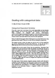
Figure 2: Similarity color map for Motivating Example.

Data Sets

Several data sets have been selected to best demonstrate various qualities and characteristics of our similarity measure Sij . Motivating Example. This is the same data set presented in Section 2.1, and is used to illustrate advantages of our technique over other similarity measures. Mushroom. This data set was selected as it contains only categorical values, and although it is a classification data set, it has also been studied in the context of clustering (Guha et al. 2000). It is obtained from the UCI Machine Learning Repository (Asuncion & Newman 2007). The original data set contains 8124 instances on 23 attributes (including the class attribute), where we removed any records with missing values. ACS PUMS. The American Community Survey (ACS) is conducted annually by the United States Census Bureau and was designed to provide a snapshot of the community. We took a random sample of 20,000 records from the 2006 Housing Records Public Use Microdata Sample (PUMS) 1 for the whole of the US. The sub-sample was chosen on only 14 attributes of the available 239, and any records with missing values on these attributes was not considered. 2.3.2

2

http://factfinder.census.gov/home/en/acs pums 2006.html

set a simple graph or a multigraph, that is, a graph with multiple edges. When showing results for the similarity measure we generally present a range of parameters for comparison. 2.3.3

Results

We present a range of results to illustrate the effectiveness of our measure. One way in which we present the similarity values is via a colour map, as shown in Figure 2. The colour map assigns different colours to different values as per the colour bar on the right hand side of the diagram. Dark red maps to 1.0 and and dark blue to 0.0. This figure shows Sij values for the Motivating Example graph on all 17 values over the 4 attributes. The parameters are as follows; T = 0.4, c1 = 0.6 and c2 = 0.4. Value S1,1 is in the bottom left hand corner of Figure 2, and value S17,17 is in the right hand top corner. If you look at the diagonal between these two values, you will see that all values along the diagonal are 1.0, since each value has maximum similarity with itself. Areas outside of an attribute are dark blue since we do not consider the similarity between values from different attributes. Motivating Example. Examining the similarity ′ ′′ values we can compare the Sij and Sij values to the scenarios discussed in Section 2.1. Table 2 gives the ′ ′′ Sij , Sij and Sij similarity values for the first attribute in our motivating example, that is, Client and shows that Vertex 5 (Mr White) and Vertex 3 (Mr Brown) ′ have no Sij similarity since they have no values in ′′ common in the data set. However, when the Sij threshold T is equal to 0.4, these two values have ′′ a Sij similarity of 1.0. This supports the notion that although these two clients do not have any direct similarity in the data set, they do have a transitive similarity which should be considered in any subsequent clustering of these values. By the appropriate assignment of values to c1 and c2 we can give the desired ′′ weight to this indirect similarity represented by Sij . In Table 2 we can see the situation for c1 = 0.6 and c2 = 0.4.

0

Proceedings of the Tenth Australasian Data Mining Conference (AusDM 2012), Sydney, Australia ′ Sij

1

2

3

4

5

6

1 2 3 4 5 6

1.000 0.667 0.000 0.000 0.000 0.000

0.667 1.000 0.000 0.000 0.000 0.258

0.000 0.000 1.000 0.333 0.000 0.258

0.000 0.000 0.333 1.000 0.667 0.258

0.000 0.000 0.000 0.667 1.000 0.515

0.000 0.258 0.258 0.258 0.516 1.000

1

2

3

4

5

6

′′

Sij 1 2 3 4 5 6 Sij 1 2 3 4 5 6

1.000 1.000 0.000 0.000 0.000 0.258 1 1.000 0.800 0.000 0.000 0.000 0.103

1.000 1.000 0.000 0.000 0.000 0.258 2 0.800 1.000 0.000 0.000 0.000 0.258

0.000 0.000 1.000 1.000 1.000 0.775 3 0.000 0.000 1.000 0.600 0.400 0.465

0.000 0.000 1.000 1.000 1.000 0.882 4 0.000 0.000 0.600 1.000 0.800 0.508

0.000 0.000 1.000 1.000 1.000 0.882 5 0.000 0.000 0.400 0.800 1.000 0.663

0.258 0.258 0.775 0.882 0.882 1.000 6 0.103 0.258 0.465 0.508 0.663 1.000

Attribute 2 − Cap Shape

Attribute 6 − Odour

6

5

6

4 4

4

3 2

2

2

1 2

4

6

Attribute 12 − Stalk Root

2

4

6

8

Attribute 13 − Stalk Surface Above Ring

4

4

3

3

2

2

1

1

2

4

6

Attribute 16 − Stalk Colour Below Ring

6 4 2 1

2

3

4

1

Attribute 19 − Ring Type 4 3 2

2

3

4

2

Attribute 21 − Population 6

6

5

5

4

4

3

3

′′

2

3

4

6

2

1 1

4

Attribute 22 − Habitat

2 1

′

Attribute 4 − Cap Colour 8

6

1 2

4

6

2

4

6

Table 2: Sij , Sij and Sij values for Client attribute in Motivating Example. Figure 3: A close look at Sij values for selected attributes in Mushroom. (T = 0.6, c1 = 0.6, c2 = 0.4). Mushroom. This data set has only categorical attributes. The results for selected attributes are presented in Figure 3 for parameters T = 0.6, c1 = 0.6 and c2 = 0.4. It can be seen from the figure that for some attributes such as Cup Shape, Cup Colour, Stalk Root and Habitat, all pairs of values exhibit similarity, while for attributes such as Stalk Colour Below Ring and Ring Type there are values which are not very similar to any other value. ACS PUMS. This data set is good mixture of categorical and numerical attributes of varying sizes. A sample of total similarity results for parameters T = 0.75, c1 = 0.6 and c2 = 0.4 are shown in Figure 4. The total similarity across all attributes is shown in the image in the top left hand corner of Figure 4, ′ ′′ while the Sij and Sij values are shown in the bottom right hand corner. There are several numerical values worth mentioning here, including the two attributes related to income, WAGP (Wages or income in the past 12 months) and PINCP (Person’s total income). Both of these attributes exhibit very numerical tendencies in that values that are close together numerically tend to be more similar than those that are further apart numerically. However, there is a noted exception to this rule for the attribute PINCP, since when the income is below zero these values have very low similarity to values just above zero, yet appear more similar to high incomes. Another attribute worth noting is Educational attainment (SCHL), in the bottom row of Figure 4. The values in this attribute appear to be partitioned into two distinct groups that have a high level of similarity within a partition, and lower similarity outside of it. The two values at the boundary of these two groups are values 8 and 9, which correspond to ‘Grade 12 no diploma’ and ‘High school graduate’ respectively. This result indicates that based on the subset of attributes in the data set, there is a strong relationship between levels of education above that of high school graduate, and also between the levels of education that fall below this benchmark. An example of a numerical attribute from the ACS PUMS data set which does not exhibit a numerical ordering is that of ‘Usual hours worked per week last 12 months’ (WKHP), shown in the top right hand

corner of Figure 4. Although there are quite a few of the values which are numerically close that also have a high level of similarity, there are also many values which do not follow this convention. In the next section we will incorporate our similarity measure into a noise addition technique for categorical values. 3

Noise Addition

In this section we propose a noise addition technique for categorical values which incorporates our similarity measure from Section 2 and uses it to cluster these values. It then assigns transition probabilities based on the discovered clusters. We also provide an analysis of experimental results to see how well our technique performs in the conflicting areas of security and data quality. Recall our Motivating Example from Section 2.1. Having evaluated the similarity values for the attributes in this data set, we are now faced with the problem of how best to partition the values so as to maximise similarity within a partition, and minimise similarity across partitions. Although it is not difficult to define a maximisation function that will indicate the quality of a selected partitioning of the graph, it is more challenging to decide how best to arrive at an optimal solution. 3.1

VICUS - Noise Addition Technique

Noise is added to a data set by applying the following three steps. Step 1: We partition the graph using the similarity measure for values within an attribute. We use a genetic algorithm to explore the solution space and arrive at a close to optimal partitioning of the graph. Step 2: Using the partitioning of the graph obtained from Step 1, we generate a transition probability matrix for all attribute values. The transition matrix gives the probabilities of each attribute value changing to every other value within the attribute.

143

CRPIT Volume 134 - Data Mining and Analytics 2012

Weighting S’ 0.6, S’’ 0.4

WAGP

PINCP

60 40

400

80

60

60

40

40

20 200

WKHP 80

100

20

20

600

20

WAOB

40

60

20

40

RAC1P

60

80

100

20

JWTR 50

8

10

40

6

8

30

6

4

4

6

8

10

2 2

4

6

8

2

4

AGEP

6

8

10

12

5

8

4

6

40

3

20

2

150

20

MAR

3

40

60

5

2

3

4

5

2

S−Prime 600

10

400

400

5

200

200

15

50

200

400

4

6

8

S−Secundum 0.75

600

10

40

2 1

15

5

30

4

SCHL

4

20

COW

1 100

10

CIT

60

80

20

4 2

60

ST

12

ANC1P

40

600

200

400

600

Figure 4: Sample results for Census PUMS data set (T = 0.75, c1 = 0.6, c2 = 0.4). Step 3: We perturb each individual value in the original data file by applying the transition probabilities. Note that the value will generally have a relatively high probability of remaining the same in the perturbed file. We next describe each of the steps in more detail. Graph Partitioning. We now define the graph partitioning problem as presented in Bui and Moon (Bui & Moon 1996). Given a graph G = (V, E) on n vertices and m edges, we define a partition P to consist of disjoint subsets of vertices of G. The cut-size of a partition is defined to be the number of edges whose end-points are in different subsets of the partition. A balanced k-way partition is the partitioning of the vertex set V into k disjoint subsets where the difference of cardinalities between the largest subset and the smallest one is at most one. The k-way partitioning problem is the problem of finding a k-way partition with the minimum cut-size (Bui & Moon 1996). We relax the condition of difference of partition sizes being at most 1, and we impose a lower bound on the minimum size of the partition minS. The k-way partitioning problem has been well studied and has been shown to be N P -complete in both the balanced and unbalanced form (Garey & Johnson 1979, Bui & Moon 1996). Hence, we will apply a heuristic, namely a genetic algorithm, to solve the problem of moving from one solution to the next. Transition Probability Matrix. When deciding how much noise to add when we perturb a data set, we must decide on how best to distribute the transition probabilities amongst the possible choices. Note that we explore two separate methods for defining

144

the transition probabilities, the first being our VICUS method, and the second being a method we term Random, which is used to evaluate the effectiveness of the VICUS method. We next describe both of them in more detail. VICUS Method. Given a partition P of the original data set which divides all possible values into k disjoint sets, we calculate the transition probabilities for each attribute individually. We use the following notation. B - the set of all values in the microdata file. P = {B1 , B2 , · · · , Bk } - a partition - a collection of disjoint subsets (some of which may be empty) of B ∪k such that i=1 Bi = B. A - the set of values of attribute A. PA = {A1 , A2 , · · · , Ak } - a partition - a collection of disjoint subsets (some of which may be empty) of A ∪k such that i=1 Ai = A and Ai ⊂ Bi , 1 ≤ i ≤ k. S - the subset from PA containing an attribute value, a ∈ A. |S| is the number of attribute values in the subset containing the value a. ′

S = PA \ S - the relative complement set containing all other subsets.

Proceedings of the Tenth Australasian Data Mining Conference (AusDM 2012), Sydney, Australia ′

|S | is the number of attribute values that are in a different subset to a. Ps - the probability of an attribute value remaining unchanged. psp - the probability that an attribute value is changed into a different attribute value from the same subset. Psp = (|S| − 1) × psp - the probability that the attribute value remains in the same subset, but not unchanged. pdp - the probability that the value a changes to a value from a different subset. ′

Pdp = |S | × pdp - the probability that the attribute value changes the subset. The transition probabilities for an attribute value a satisfy the following; Ps + Psp + Pdp = 1

(5)

We now introduce two parameters that allow the data manager to adjust the amount of noise to be added to the microdata file. The first parameter, k1 , is defined such that an attribute value a is k1 times more likely to stay the same than to change to another value in the same subset. The second parameter, k2 , tells us how many times more likely a value a is to change to another in the same subset than one in a different subset. Hence, we can reformulate our probabilities as Ps = k1 × psp = k1 × k2 × pdp

(8)

and Equation 5 becomes Ps + (|S| − 1) ×

′ Ps Ps + |S | × =1 k1 k1 × k2

(9)

From the above, the probability that a value remains the same becomes Ps =

3.1.1

k1 × k2 k1 × k2 + k2 × (|S| − 1) + |S ′ |

(9)

pdp =

1 k1 × k2 + k2 × (|S| − 1) + |S ′ |

(10)

psp =

k2 k1 × k2 + k2 × (|S| − 1) + |S ′ |

(11)

Random Method

We also define a set of transition probabilities for the method we term Random. This method does not assign probabilities for Psp and Pdp , but rather introduces the probability of a value changing to any other value in the attribute, which is denoted Pc . However, it still uses Equation 9 to calculate the probability of a value remaining unchanged in the perturbed data set. We define the probability of a value changing to any other value in the attribute as follows Pc =

1 − Ps |S| + |S ′ | − 1

(12)

The resulting method will perform better than a truly random method, as it is imparting some of the information from our partitioning of the values when calculating the value for Ps . However, to evaluate the quality of our method we need to perturb the ‘random’ in such a way as to be able to compare the results of our security measure and data quality tests. Perturbing Microdata File. Once the transition probability matrix has been generated for each attribute, the next step is to simply perturb the original microdata file according to the transition probabilities assuming that a random value is drawn to decide if the value changes to another value in the same partition, one from a different partition, or remains unchanged. 3.2

Evaluation Methods

We now evaluate VICUS both in terms of security and data quality. In evaluating the security of a perturbed data set we assume that the intruder is aware of the exact perturbation technique. We apply an information theoretic entropy (Shannon 1948) measure to estimate the amount of uncertainty the intruder has about the identity of a record as well as the value of a confidential attribute. In order to gauge how well our noise addition technique preserves the underlying data quality, we apply the chi-square statistic test. Input: Transition Probability matrix M , Perturbed microdata file P , Probabilities px for all records Output: H(D) entropy for each value ci ∈ C do initialise probability Di to 0; end for each record x in P with Cx for C do for each confidential value in ci ∈ C do /* Sum the probability that Cx in P originated from ci */ /* in O and multiply by the probability that */ /* record x is the record the intruder ‘knows’ */ Di + = p(ci = O(Cx )) × px ; end end /* Now calculate the entropy of the confidential value Vc */ ∑|C| 1 H(D) = 1 Di log2 Di ; return H(D); Algorithm 2: Calculating entropy of confidential attribute in perturbed microdata file. Security Measure. One way in which we can measure the security of a released microdata file is by estimating how certain an intruder is that they have identified a record, and more importantly the correct confidential value for that record (Oganian & Domingo-Ferrer 2003). To gauge the amount of uncertainty an intruder has about having identified a particular record in the perturbed microdata file, we calculate the entropy for this record. Similarly, by calculating the entropy of a confidential value we can estimate the amount of uncertainty the intruder has about this value. We assume that there is only one confidential or sensitive attribute in the microdata file; it is straightforward to generalise to a case where there is more than one confidential attribute. We assume that an intruder (1) knows how noise has been added to the microdata file (2) knows one or more

145

CRPIT Volume 134 - Data Mining and Analytics 2012

attribute values about a particular record for which they wish to learn the confidential value (3) only has access to the perturbed and not the original microdata file (4) is trying to compromise one particular record in the database and that they know the original values of some or all non-confidential attributes for that record. The algorithm used to calculate the entropy of a confidential attribute is given in Algorithm 2. Data Quality. Information loss is an important consideration when evaluating the quality of a perturbation technique (Trottini 2003). The goal of the data manager is to minimise the reduction in data quality while at the same time maximise the security of released data. In order to evaluate how VICUS performs in terms of information loss apply a chi-square statistical test to both the original and perturbed data sets to ascertain how successfully VICUS preserves the underlying statistics from the original data set. The chi-square test is a commonly applied statistical measure for determining the statistical significance of an association between two categorical attributes (Utts & Heckard 2004). We follow the five step approach to determining statistical significance as outlined by Utts and Heckard (Utts & Heckard 2004, p.184). Note that our aim here is not to determine if there is any statistical significance of the attribute associations studied, rather we aim to determine that any such significance is undisturbed by our perturbation method. Mushroom Comparing entropy to the number of attribute known to the intruder VICUS (k1=2, k2=20) Random (k1=2, k2=20) VICUS (k1=10, k2=50) Random (k1=10, k2=50)

12

11

10

entropy

9

8

7

6

5

4

3 2

4

6

8 10 12 14 number of attributes known to the intruder

16

18

20

Figure 5: Record entropy vs number of known attributes, Mushroom data set. We analyse our data set in the form of two-way contingency tables, which count the co-occurrence of a categorical value from one attribute with a value in another attribute, for all combinations of values. Since we are dealing with categorical data specifically, and all of our experimental data sets have been perturbed under this assumption, the chi-square statistic is a natural choice. The chi-square statistic, χ2 , measures the difference between the observed counts in the contingency table and the so-called expected counts, which are those that would occur if the there was no relationship between the two categori-

146

cal variables (Utts & Heckard 2004). An alternative statistic is the Likelihood Chi-Square χ2LR was also used in our analysis. For large data sets the values of χ2 and χ2LR should be comparable. The same method is used to compare these statistics to the p-value to evaluate the correctness of the null hypothesis. 3.3

Experiments - Noise Addition

From the data sets examined in Section 2.3, where we looked at experimental results for our similarity measure, we present only the results for the Mushroom Data Set in this paper. In preparing our experiments we generated a multigraph from the original data set, and we ran a genetic algorithm 30 times and selected the partition with the largest fitness function. We next select five different combinations of parameters for the transition probability generation, and for each selection we perturbed 30 files according to the generated transition probabilities. Security. We calculated the entropies for the situation when the user knows one, two, three and all of the attributes excluding the confidential one, to give a comparison ‘worst case scenario’ result. For each of the 30 perturbed files, we averaged the entropies over all records and all files for when the intruder knows one attribute value, and present the results in Table 3. The average entropies do not differ significantly between VICUS and Random method and the range between 11 and 12 bits for record entropy and 1.6 and 2.6 bits for confidential attribute entropy. In Figure 5 we show how the entropy drops when the user learns more attribute values for a particular record. We are also interested to know if certain attributes are more or less revealing than others, that is, if they yield a lower or higher entropy than average. Figure 6 provides a close up view of the entropies for each individual attribute. Data Quality. We used the SPSS Statistical Software package to analyse the Chi-square statistics of the mushroom data set. For each attribute pair we calculated the Pearson’s Chi-Square statistic and Likelihood Ratio Chi-Square statistic on the original data set, 30 files perturbed using VICUS method and 30 file perturbed via the Random method. We compared both the Chi-square statistic value and associated p-value for each. We first want to see VICUS performed in terms of how far the χ2 values were from those on the original file and the Randomly perturbed files. We next wanted to verify if there was a change in the outcome of the null hypothesis for the files perturbed with the VICUS method. We chose to look at Attribute 4 (Cap Colour ) against the other attributes, since this attribute showed to be the most sensitive in terms of security when we calculated the entropy for the user knowing one attribute value (Figure 6). We also selected only a single combination of values for the parameters, namely k1 = 5 and k2 = 20, as this combination gave middle of the range results on entropy. Of the 21 attribute combinations, there were 7 attribute pairs that satisfied the large sample requirement on the original data set. That is, these attributes had over 80% of cells in the contingency table with expected counts larger than 5, and all cells had an expected count larger than 1. Figure 7 compares the distributions of the χ2 statistic values for the 30 files perturbed via the VICUS and Random methods, and shows how far away they are from the χ2 statistic for the original file,

Proceedings of the Tenth Australasian Data Mining Conference (AusDM 2012), Sydney, Australia

Perturbation

k1

k2

Mush1 Mush2 Mush3 Mush4 Mush5

2 5 10 10 10

20 20 10 20 50

VICUS Random Record Entropy 11.9720 12.0074 11.7502 11.7316 11.6141 11.5772 11.5826 11.5487 11.5567 11.5284

VICUS Random Confidential Entropy 2.0743 2.4496 1.8778 2.1962 1.8280 2.0036 1.7220 1.9450 1.6409 1.9045

Table 3: Average record and confidential attribute entropy.

Mushroom − Mush5 Record entropy for VICUS and Random Intruder knows 1 particular attribute

Comparing Chi−Square Statistic Distributions 8 VICUS Random maximal entropy 7

12.5 12.3

6

12.1 11.9

5

Support

entropy

11.7 11.5

4

11.3 3

11.1 10.9

2

10.7 10.5

1

1

2

3

4

5

6

7

8

9

10 11 12 13 attribute number

14

15

16

17

18

19

20

21

22

0

0

500

1000 1500 Pearson’s Chi−Square Statistic

2000

2500

Figure 6: Record entropy sensitivity.

Figure 7: Chi-square statistic

which had the value of 2711.8. For all 30 files VICUS had the χ2 greater that 1500, while Random had the χ2 value less than 1000. On all attribute pairs examined, our VICUS method produced χ2 values closer to the original than the those of the random method.

of security and data quality. We observed that a low value for k1 and high value for k2 transition probability parameters lead to improved performance in terms of both data quality and security of VICUS over the Random method. Setting the product (k1 × k2 ) of these parameters to a value of 100 or higher, while also ensuring that k1 is low and k2 is high appears to give the best balance between the conflicting goals of security and data quality.

4

Conclusion

In this paper we have presented a new noise addition technique, VICUS, for application on categorical data. The first step of VICUS is to calculate the similarity between the categorical attribute values. To this end we have designed a new similarity measure specifically for use on categorical attribute values. The similarity measure aims to capture the notion of transitive similarity between values of an ′′ attribute, the so called S similarity. As the results of experimental analysis show, our similarity measure is effective in capturing the similarities that occur in the microdata when values no neighbours in common. Although VICUS is designed for application on categorical values, it can also be applied to numerical attributes by treating the discrete values as categories. The experiments showed that not all numerical attributes exhibit a numerical ordering according to our similarity measure, that is, values that are numerically close together do not necessarily have a high similarity. This would seem to indicate that the application of traditional numerical noise addition techniques on such attributes could result in reduced quality of the perturbed data set. Experimental results indicate that VICUS performs well in both the areas

References Asuncion, A. & Newman, D. (2007), ‘UCI machine learning repository’. URL: http://www.ics.uci.edu/∼mlearn/MLRepository.html Brankovic, L. & Estivill-Castro, V. (1999), Privacy issues in knowledge discovery and data mining, in ‘Proceeding of the Australian Institute of Computer Ethics, AICE99’, Lilydale, Melbourne, Australia. Brankovic, L. & Giggins, H. (2007), Security, Privacy and Trust in Modern Data Management, Springer, New York, chapter Statistical Database Security, pp. 167–182. Brankovic, L., Hor´ak, P. & Miller, M. (2000), ‘An optimization problem in statistical databases.’, SIAM J. Discrete Math. 13(3), 346–353. Brankovic, L., Horak, P., Miller, M. & Wrightson, G. (1997), Usability of compromise-free statistical databases for range sum queries, in ‘Proceed-

147

CRPIT Volume 134 - Data Mining and Analytics 2012

ing of Ninth International Conference on Scientific and Statistical Database Management, IEEE Computer Society’, August 11-13, Olympia, Washington, pp. 144–154. Brankovic, L., Islam, M. Z. & Giggins, H. (2007), Security, Privacy and Trust in Modern Data Management, Springer, New York, chapter Privacy Preserving Data Mining, pp. 151–165. Brankovic, L. & Miller, M. (1995), ‘An application of combinatorics to the security of statistical databases’, Australian Mathematical Society Gazette 22(4), 173–177. ˘ an Brankovic, L., Miller, M. & Sir´ ˘, J. (1996b), ‘Graphs, 0-1 matrices, and usability of statistical databases’, Congressus Numerantium 12, 196–182. ˘ an Brankovic, L., Miller, M. & Sir´ ˘, J. (2002), ‘Range query usability of statistical databases’, Int. J. Comp. Math. 79(12), 1265–1271. ˇ an Brankovic, L., Miller, M. & Sir´ ˇ, J. (1996a), Towards a practical auditing method for the prevention of statistical database compromise, in ‘Proceeding of Australasian Database Conference’. ˘ an Brankovic, L. & Sir´ ˘, J. (2002), 2-compromise usability in 1-dimensional statistical databases, in ‘Proc. 8th Int. Computing and Combinatorics Conference, COCOON2002’. Brickell, J. & Shmatikov, V. (2008), The cost of privacy: destruction of data-mining utility in anonymized data publishing, in ‘KDD ’08: Proceeding of the 14th ACM SIGKDD international conference on Knowledge discovery and data mining’, ACM, New York, NY, USA, pp. 70–78. Bui, T. N. & Moon, B. R. (1996), ‘Genetic algorithm and graph partitioning’, IEEE Transactions on Computers 45(7), 841–855. Dwork, C. (2006), ‘Differential privacy’, Lecture Notes in Computer Science 4052, 1–12. Dwork, C., McSherry, F., Nissim, K. & Smith, A. (2006), Calibrating noise to sensitivity in private data analysis., in ‘Proceedings of Third Theory of Cryptography Conference, TCC 2006’, New York, NY, USA, pp. 265–284. Estivill-Castro, V. & Brankovic, L. (1999), Data swapping: Balancing privacy against precision in mining for logic rules, in ‘Proceedings of Data Warehousing and Knowledge Discovery, DaWaK99’, Florence, Italy, pp. 389–398.

Griggs, J. R. (1997), ‘Concentrating subset sums at k points’, Bulletin Institute Combinatorics and Applications 20, 65–74. Griggs, J. R. (1999), ‘Database security and the distribution of subset sums in Rm ’, J´ anos Bolyai Math. Soc. 7, Graph Theory and Combinatorial Biology pp. 223–252. Guha, S., Rastogi, R. & Shim, K. (2000), ‘Rock: A robust clustering algorithm for categorical attributes’, Information Systems 25(5), 345–366. URL: citeseer.ist.psu.edu/guha00rock.html Horak, P., Brankovic, L. & Miller, M. (1999), ‘A combinatorial problem in database security’, Discrete Applied Mathematics 91(1-3), 119–126. Islam, M. Z. & Brankovic, L. (2005), Detective: A decision tree based categorical value clustering and perturbation technique in privacy preserving data mining, in ‘Proceedings of the 3rd International IEEE Conference on Industrial Informatics (INDIN 2005)’, Perth, Australia. Islam, M. Z. & Brankovic, L. (2011), ‘Privacy preserving data mining: A noise addition framework using a novel clustering technique’, Knowledge-Based Systems 24, 1214–1223. Li, N., Li, T. & Venkatasubramanian, S. (2007), t-closeness: Privacy beyond k-anonymity and ldiversity, in ‘Proceedings of IEEE 23rd International Conference on Data Engineering, 2007. ICDE 2007.’, pp. 106–115. Machanavajjhala, A., Kifer, D., Gehrke, J. & Venkitasubramaniam, M. (2007), ‘L-diversity: Privacy beyond k-anonymity’, ACM Trans. Knowl. Discov. Data 1(1), 3. Muralidhar, K. & Sarathy, R. (2003), ‘A theoretical basis for perturbation methods’, Statistics and Computing 13, 329–335. Oganian, A. & Domingo-Ferrer, J. (2003), ‘A posteriori disclosure risk measure for tabular data based on conditional entropy’, SORT - Statistics and Operations Research Transactions 27(2), 175–190. Samarati, P. & Sweeney, L. (1998), Protecting privacy when disclosing information: k-anonymity and its enforcement through generalization and suppression, in ‘Proceedings of the IEEE Symposium on Research in Security and Privacy’, Oakland, California, USA. Shannon, C. E. (1948), ‘A mathematical theory of communication’, Bell Syst. Tech J. 27, 379–423.

Garey, M. R. & Johnson, D. S. (1979), Computers and intractability: A guide to the theory of N P completeness, W. H. Freeman and Company, San Francisco.

Sweeney, L. (2002), ‘k-anonymity: a model for protecting privacy. international journal on uncertainty’, International Journal on Uncertainty, Fuzziness and Knowledge-based Systems 10(5), 557–570.

Giggins, H. & Brankovic, L. (2002), Ethical and privacy issues in genetic databases, in ‘Proceedings of the Third Australian Institiute of Computer Ethics Conference’, Sydney, Australia.

Trottini, M. (2003), Assessing disclosure risk and data utility: A multiple objectives decision problem, in ‘Joint ECE/Eurostat Work Session on Statistical Confidentiality’, Luxembourg.

Giggins, H. & Brankovic, L. (2003), Protecting privacy in genetic databases, in R. L. May & W. F. Blyth, eds, ‘Proceedings of the Sixth Engineering Mathematics and Applications Conference’, Sydney, Australia, pp. 73–78.

Utts, J. M. & Heckard, R. F. (2004), Mind on statistics, 2nd edn, Thomson-Brooks/Cole, Belmont, Calif.

148

Willenborg, L. & de Waal, T. (2001), Elements of Statistical Disclosure Control, Lecture Notes in Statistics, Springer, New York, USA.