Electronic Journal of Statistics Vol. 7 (2013) 1369–1386 ISSN: 1935-7524 DOI: 10.1214/13-EJS810
PPtree: Projection pursuit classification tree Yoon Dong Lee† Business school, Sogang University, Seoul, Korea
Dianne Cook Department of Statistics, Iowa State University, Ames, IA, USA
Ji-won Park and Eun-Kyung Lee∗ Department of Statistics, Ewha Womans University, Seoul, Korea e-mail:
[email protected] Abstract: In this paper, we propose a new classification tree, the projection pursuit classification tree (PPtree). It combines tree structured methods with projection pursuit dimension reduction. This tree is originated from the projection pursuit method for classification. In each node, one of the projection pursuit indices using class information - LDA, Lr or PDA indices - is maximized to find the projection with the most separated group view. On this optimized data projection, the tree splitting criteria are applied to separate the groups. These steps are iterated until the last two classes are separated. The main advantages of this tree is that it effectively uses correlation between variables to find separations, and it has visual representation of the differences between groups in a 1-dimensional space that can be used to interpret results. Also in each node of the tree, the projection coefficients represent the variable importance for the group separation. This information is very helpful to select variables in classification problems. Keywords and phrases: Classification tree, projection pursuit, variable selection. Received August 2012.
Contents 1 Introduction . . . . . . . . . . . . . . . . . . 2 Exploratory projection pursuit classification 2.1 The general procedures for PPtree . . 2.2 Illustration: Iris data . . . . . . . . . . 2.3 Main features of PPtree . . . . . . . . 2.4 Variable selection and importance . .
. . . tree: . . . . . . . . . . . .
. . . . . PPtree . . . . . . . . . . . . . . . . . . . . .
. . . . . .
. . . . . .
. . . . . .
. . . . . .
. . . . . .
. . . . . .
1370 1371 1371 1372 1374 1375
∗ This research was supported by Basic Science Research Program through the National Research Foundation of Korea(NRF) funded by the Ministry of Education, Science and Technology(2010-0003840). † This work was supported by the Sogang University Research Grant of 201210023.01.
1369
1370
Y. D. Lee et al.
3 Applications . . . . . . . . . . . . . . . . . . . . . . . 3.1 Australian Crab data . . . . . . . . . . . . . . . 3.2 Three gene expression datasets . . . . . . . . . 4 Variable selection with PPtree . . . . . . . . . . . . 4.1 Wine identification data . . . . . . . . . . . . . 4.2 Glass identification data . . . . . . . . . . . . . 5 Comparison of performance with tree-based methods 6 Discussion . . . . . . . . . . . . . . . . . . . . . . . . Acknowledgements . . . . . . . . . . . . . . . . . . . . . References . . . . . . . . . . . . . . . . . . . . . . . . . .
. . . . . . . . . .
. . . . . . . . . .
. . . . . . . . . .
. . . . . . . . . .
. . . . . . . . . .
. . . . . . . . . .
. . . . . . . . . .
. . . . . . . . . .
. . . . . . . . . .
1376 1376 1380 1381 1381 1382 1383 1385 1385 1385
1. Introduction Projection pursuit is a method to find interesting low-dimensional linear projections of high-dimensional data by optimizing some pre-determined criterion function, called a projection pursuit index. This idea originated with Kruskal ([1]), and Friedman and Tukey ([2]) coined the term “projection pursuit” as a technique for exploring multivariate data. It is useful in an initial data analysis. The method also can be used to reduce multivariate data to a low dimensional but “interesting” sub-space. Several projection pursuit indices for classification have been proposed: LDA, Lr ([3]) and PDA ([4]) indices. The PDA index is useful for the large p, small n problems. These indices can also be used to select variables that are important to separate classes, which can help to build a better classifier. Classification trees are classifiers that use single variables to build a classification but be improved from using new variables derived by projection pursuit. The first tree algorithm was THAID ([5, 6]). Then, C4.5 ([7]) and CART ([8]) were developed. CART is implemented in R [9] as rpart [10] and it is still popular for data mining. Based on the Fast Algorithm for Classification Trees (FACT) ([11]), new algorithms for tree fitting, CRUISE ([12]), GUIDE ([13]), and QUEST ([14]) have greatly extended the original methods. CHAID ([15]) is a tree structured method for categorical or categorized data. In most applications, the goal is to have a simple tree model that is also highly accurate for classification. Most of tree structured methods use binary splits with one variable in each node. After building the tree, expansively, pruning is used to make the tree simple. The advantage of a tree classifier is that it is easy to understand and interpret. Some methods, for example CRUISE, allow multi-way splits and linear combinations of variables to accommodate correlation between variables and to improve accuracy. CRUISE generates new variables, available for splitting, using linear discriminant analysis methods. This new proposed algorithm, the projection pursuit classification tree (PPtree), uses projection pursuit to find good low-dimensional projections revealing separations between classes, and uses these as variables for splitting, to build a more simply structured tree where there is correlation between the original variables. This new method is also helpful to understand how the class structure
PPtree
1371
relates to the measured variables and can provide a graphical representation for verifying the supervised classification results. For multivariate data with class information, it is important to have a classifier which is easy to understand that can represent the result graphically in a low-dimensional space. Therefore, it is important to find the optimal projections of the separated classes. At each node, the PPtree will separate data into two subsets, based on linear combinations of the variables. It can help to find the important variables to separate two groups from several classes. This article is organized as follows. In Section 2, PPtree algorithm is describes in detail. Section 3 illustrates the use of PPtree for several applications. In Section 4, variable selection using PPtree is shown. A discussion of future directions, strengths and weaknesses follows. 2. Exploratory projection pursuit classification tree: PPtree This section describes how to construct a PPtree and how to classify data using it. 2.1. The general procedures for PPtree The PPtree uses a recursive binary partition method. Construction of the PPtree For the data set, (Xi , yi ), where Xi is a vector with exploratory variables in p-dimensional space, yi represents class information of Xi , yi ∈ {1, 2, . . . , G}, and i = 1, . . . , n, 1. Find the optimal one-dimensional projection, α∗ , for separating all classes in the current data. 2. Reduce the number of classes to two, by comparing means, and assign a new label “G1” or “G2”(yi ∗ ) to each observation. 3. Re-do projection pursuit with these new group labels, “G1” and “G2”, finding the optimal one-dimensional projection, α, using (Xi , yi ∗ ). 4. Calculate the decision boundary c. 5. Keep α and c. 6. Separate data into two groups using new group labels “G1” and “G2”. 7. For “G1” group, (a) If there is only one class among the original classes {1, 2, . . . , G}, stop expanding the PPtree. (b) Else, repeat repeat step 1 through step 6 with the se classes. 8. For “G2” group, (a) If there is only one class among the original classes {1, 2, . . . , G}, stop expanding the PPtree. (b) Else, repeat step 1 through step 6 with the se classes.
1372
Y. D. Lee et al.
In step 1, several projection pursuit indices for classification can be used, for example, LDA, Lr or PDA indices ([3] and [4]). If there are a large number of variables relative to the sample size (large p, small n problem), the PDA index is recommended. After finding the optimal one-dimensional projection α∗ , project all the data onto α∗ . This is the most separable one-dimensional view for the chosen projection pursuit index. In this view, the means of each class is calculated and used make reduce from G to 2 groups using the distances among the means of classes. For example, if we have 5 classes and their means of the projected data in each class are 2.1, 2.3, 2.5, 3.5, and 3.7, the classes with mean 2.1, 2.3, and 2.5 are assigned to the group “G1” and the classes with mean 3.5 and 3.7 are assigned to the group “G2”. The groups “G1” and “G2” could contain one or more of the original classes. In the step 3, find the optimal one-dimensional projection α with new group information “G1” and “G2”. This step is to find the best separation of “G1” and “G2” upon which to make the decision rule for the current node. The data is split into two groups using binary partition. If αT M1 < c, then assign “G1” group to the left node. Else, assign “G2” group to the right node, where M1 is the mean of “G1” group. With this one split rule, the data can be split into two groups. For each group, we can apply step 1 through step 6 recursively, until group “G1” and “G2” have only one class from the original {1, 2, . . . , G} classes. 2.2. Illustration: Iris data To help explain PPtree algorithm, we illustrate the process using the famous Fisher’s Iris data([17]). In the Iris data (Figure 1), there are 4 variables (sepal length, sepal width, petal length and petal width) and 3 classes (Setosa, Versicolour, and Virginica). Each class has 50 observations. In Figure 1, Setosa class can be separated from the other two classes with petal length variable. Versicolour and Virginica classes are separable within the plot of petal length and petal width. In this data, the LDA index is used to find the optimally separated projections. Complete step 1, find the optimal one-dimensional projection α∗1 for three classes. Figure 2 shows a histogram of the data projected onto this optimal one-dimensional projection α∗1 : “1” represents Setosa class, “2” represents Versicolour class and “3” represents Virginica class. From the histogram, it can be seen that the centers of Versicolour class and Virginica class are much closer than the center of the Setosa class. Therefore, the two groups are “Setosa” and “Versicolour and Virginica”, which are assigned “G1” and “G2” respectively (step 2). Step 3 is to find a new optimal one-dimensional projection α1 using the reduced class labels, “G1” and “G2”. Figure 3 shows the histogram of the projected data onto this optimal one-dimensional projection α1 : “1” represents “G1” group and “2” represents “G2” group. The separation of these two groups is slightly better than the original one in Figure 2. On this projection, splitting
PPtree
1373
Fig 1. Iris data: scatterplot matrix with 4 variables. There are 3 classes, Setosa (red ◦), Versicolour (green △), and Virginica (blue +).
decisions are made; If αT1 X ≥ c1 , then assign X to the right node, else, assign X to the left node. The PPtree structure for step 1 through step 6 is drawn in the right plot of Figure 3. In this tree, the left node has only one class, “1”, therefore that node will be a terminal node (step 7(a)). In the right node, there are two classes, “2” and “3”, and this node needs more work in order to separate classes “2” and “3” (step 8(b)). Repeat step 1 through step 6 with only data in class “2” and “3”. In step 1, the optimal one-dimensional α∗2 is found. Figure 4 is the histogram of the projected data onto α∗2 . In this plot, “3” represent Virginica class and “2” represents Versicolour class. Because we have only two classes, we can assign “G1” to class “3” and assign “G2” to class “2” in step 2. We also can skip step 3 and set α2 as α∗2 . The decision rule is made; If αT2 X ≥ c2 , then assign X to the right node. If else, assign X to the left node. Applying this decision rule, the right and
1374
Y. D. Lee et al.
Fig 2. Steps 1, 2, and 3 illustrated with the iris data. At left is the best one-dimensional projection, where three classes are visible. At right, classes 2, 3 are grouped together for the tree split.
Fig 3. Steps 4, 5, and 6 illustrated with the iris data. At left is the new optimal projection, and split position. At right is a representation of the PPtree result at the end of this step.
left nodes are almost pure, so both nodes are considered to be terminal nodes. The final tree structure with decision rules is represented in the right side of Figure 4. 2.3. Main features of PPtree There are several outstanding features of the PPtree classifier. Sometimes treebased classification methods produce very large, complex trees. These complex trees are simplfied by pruning. However, it is still a complicated tree, even though there may be few classes. This is because most algorithms work variable by variable, and if the separation falls in a linear combination of variables the
PPtree
1375
Fig 4. Final result of PPtree on the Iris data: Separation in N2 node and the final tree structure. The separation between the three classes is extemely good.
algorithm has to do a lot of work to capture it. In contrast, PPtree produces a simple tree. Moreover if a linear boundary exists in the data, PPtree produces a tree without misclassification. At each node, the PPtree separates two classes using a linear combination. The number of classes will be the same as the number of final nodes, so the depth of tree is at most G − 1 (G is the number of classes). It doesn’t need pruning. In addition, at each node, it is possible to make a histogram of the projected data which can be used to study the separation. Thus, the reasons for any misclassifications can be examined at each node. Another important feature of PPtree is that it can be used to the variable selection problem. We will discuss this feature in the next subsection. 2.4. Variable selection and importance Understanding the tree takes a little more work than a regular tree. The variables need to be standardized before computing the PPtree, so that the projection coefficients can be used to interpret the contributions of the variables. After constructing the PPtree, an extra step is required to understand the contribution of the variables at each node. In node N1 (Figure 4), the PPtree uses the projection (α1 ) and separates “1” from the other two classes. Figure 5 (left) shows the absolute values of the coefficient in α1 . Petal length has the largest contribution and petal width contributes about half as much. This tells us that petal length, primarily, and petal width, secondarily, have an important role in separating “1” (Setosa) from the other two classes. Figure 5 (right) shows the absolute values of the coefficient in the projection α2 that separates “2” from “3” in node N2. This is a more equal combination of the same two variables, petal length and petal width, with a small, but perhaps significant, contribution from
1376
Y. D. Lee et al.
Fig 5. (Left) Absolute value of the projection coefficients, α1 , in the node N1, which separates “Setosa” from “Versicolour and Virginica”. (Right) Absolute value of the projection coefficients, α2 , in the node N2, which separates “Versicolour” from “Virginica”. The same two variables have prominent contributions to both projections, stressing their importance for the separation of all three classes, but the linear combination of the variables differs slightly, and borrows a little from a third variable to separate “Versicolour” from “Virginica”.
sepal length. This says that the same two variables are of primary importance for separating all three classes, with sepal length having some contribution to separating the latter two classes. This is an important feature of PPtree. In each node, PPtree separates classes into two groups using the optimal one-dimensional projections. The absolute values of coefficients of the optimal projection can be interpreted as the amount of contribution from each variable toward separating the classes. Variables with the larger coefficient values play an important role in separating the two groups. Therefore, we can determine the important variables in each separation. Information about variable contribution at each node can be used to define a new importance measure, which we call the PPtree importance measure (PPtreeIM). PPtree-IM is the weighted average of the absolute value of the projection coefficients. The weights take the number of classes in each node into account. We will show how this measure works in Section 4 with two real examples. 3. Applications 3.1. Australian Crab data This dataset ([18]) contains information on 200 crabs from 2 species (Blue and Orange). Each species has 50 females and 50 males, resulting in 4 groups BF (Blue-Female), BM (Blue-Male), OF (Orange-Female) and OM (Orange-Male). There are 5 continuous variables: the carapace length (CL) and width (CW), the size of the frontal lobe (FL), rear width (RW), and the body depth (BD). Figure 6 shows the scatterplot matrix of this crab data. It is hard to separate the 4 classes using these 5 variables because separation between groups is only in combinations of the variables. CART produces a complicated decision tree where variables are used multiple times, and the accuracy is poor. This is a
PPtree
1377
Fig 6. Australian Crab data: scatterplot matrix with 5 variables. There are 4 classes, BlueFemale (BF: red ◦), Blue-Male (BM: green △), Orange-Female (OF: blue +), and OrangeMale (OM: pink ×).
situation where PPtree performs well. Figure 7 and Figure 8 show the result of CART, and PPtree using the LDA index. The tree structure from CART (Figure 7) is very complex and even though this tree is complex, 45 crabs out of 200 crabs are misclassified. Figure 8 is the result from PPtree. It is very simple and only 6 crabs are misclassified with this tree. To understand the contribution of the variables to the separations the projections used at each node are examined. In node N1, the Blue species (BF:1 and BM:2) is separated from the Orange species (OF:3 and OM:4). Figure 9 displays a histogram of the projected data in node N1 and the coefficients of optimal projections. From the histogram of the projected data in node N1, it can be seen that there are no misclassified crabs in this separation. Therefore the Blue and Orange species are clearly separated in node N1. The absolute value of the coefficient corresponding to the variable CW is the largest and it is contrasted by a combination of FL, CL and BD.
1378
Y. D. Lee et al.
Fig 7. Results of CART on the Australian Crab data: This tree result is very complex, and worse, more than 20% of data are misclassified.
Fig 8. Results of PPtree on the Australian Crab data: This tree is very simple and only 6 crabs (3%) are misclassified.
Fig 9. Interpreting the results of PPtree on the Australian crab data at Node 1 (N1): projected data and projection coefficients, 1=Blue Female (BF), 2=Blue Male (BM), 3=Orange Female (OF), 4=Orange Male (OM). In this node, the two species are separated, and CW has an important role in this separation.
PPtree
1379
Fig 10. Interpreting the results of PPtree on the Australian crab data at Node 2 (N2): projected data and projection coefficients, 3=Orange Female (OF), 4=Orange Male (OM). In the Orange species, males and females are separated, and CL contrasted with RW has an important role.
Fig 11. Interpreting the results of PPtree on the Australian crab data at Node 3 (N3): projected data and projection coefficients, 1=Blue Female (BF), 2=Blue Male (BM). In the Blue species, males and females are separated. Similarly to the Orange species, CL and RW also have an important role in this separation.
Females and males of the Orange species are separated in node N2. They are not clearly separated. Figure 10 displays a histogram of the projected data in node N2 and the coefficients of optimal projections. The coefficients of the projection indicate that this is effectively a contrast between variables RW and CL, which means that the difference between males and females is that females have small CL values relative to large RW value. Also it can be seen that males CW have small values on the projection and females large values. Two female crabs in Orange species are misclassified. Node N3 separates females and males of the Blue species. Figure 11 displays a histogram of the projected data in node N2 and the coefficients of optimal projections. The type of separation is similar to that of the Orange species. The projection is basically a contrast of RW and CL. Although, for this species the variable FL also has a substantial contribution. Three male crabs in Blue species and one female crab in Blue species are misclassified.
1380
Y. D. Lee et al.
Using PPtree, it is possible to understand the special characteristics of each group with respect to the classes. It is possible to see which cases are misclassified and the reason why this happens, in each node, using the histogram of the projected data and the values of projection coefficients. 3.2. Three gene expression datasets Three gene expression datasets are used to examine the performance of PPtree relative to other classifiers: Leukemia, Lymphoma and NCI60 [19]. The Leukemia data consists of 25 cases of AML, 38 cases of B-cell ALL, and 9 cases of T-cell ALL. After preprocessing, 3571 gene expression values are available. The Lymphoma dataset consists of 29 cases of B-cell chronic lymphocytic leukemia (B-CLL), 9 cases of follicular lymphoma (FL), and 42 cases of diffuse large B-cell lymphoma (DLBCL). After preprocessing, 4682 gene expression values are avaiable. The NCI60 dataset consists of eight different tissue types: 9 cases of breast, 5 cases of central nervous system (CNS), 7 cases of colon, 8 cases of leukemia, 8 cases of melanoma, 9 cases of non-small-cell lung carcinoma (NSCLC), 6 cases of ovarian, and 9 cases of renal. There are 6830 genes. Dudoit et al. [19] compares several discrimination methods with these three datasets. PPtree is compared with the results from [19]. First, the rule used in [19] to select genes from each dataset is applied. We select 40, 50 and 30 genes from Leukemia, Lymphoma, and NCI60 data, respectively, using the ratio of between-group to within-group sums of squares. A 2/3 training set is generated, and the PPtree is built with two different PP indices, LDA and PDA. The test error is calculated using the 1/3 test set. The whole procedure is repeated 200 times, and the median and upper quantile of test errors is calculated, and compared across methods. The results are in Table 1. In the Leukemia dataset, the best classifier was the diagonal linear discriminant analysis (DLDA) and the worst classifier was Fisher’s linear discriminant analysis (FLDA) in [19]. The median error of the best one is 1 and the worst shows 3 errors among the 24 cases in the test set. PPtree with LDA index shows 2 errors which is between the best result and the worst result in [19]. On the other hand, PPtree with PDA index(λ = 0.5) shows the similar result(1 error) as the best classifier, DLDA. In the Lymphoma dataset, diagonal quadratic disTable 1 Comparison of PPtree results with previous classification results of the three gene expression datasets. The median and upper quartile of test errors from 200 re-samples are shown Leukemia Method Q2 Best/Worst Predictor ∗ DLDA 1 FLDA 3 PPtree LDA index 2 PDA index 1
Q3 2 4 3 1
Lymphoma Method Q2 DQDA FLDA
0 6
Q3 1 8
4 5 2 3 ∗ Results from Dudiot et al. (2001)
NCI60 Method Q2
Q3
DLDA CV
7 12
8 13
10 6
11 8
PPtree
1381
criminant analysis (DQDA) shows the best result (0 error) and FLDA shows the worst result (6 errors). PPtrees with both indices work better than FLDA, but worse than DQDA. In the NCI60 dataset, the diagonal quadratic discriminant analysis (DQDA) shows the best result (7 errors) and the cross validation (CV) shows the worst result (12 errors). PPtree with PDA index shows 6 errors. It is the best result among the other discriminant methods in [19]. PPtree with LDA index shows better performance than CV and worse than DLDA. In comparison to these previous analyses of the three gene expression datasets, the accuracy of the PPtree is very competitive. 4. Variable selection with PPtree Two datasets, wine and glass, are used to show how PPtree works for variable selection. These two datasets are from the UCI Machine Learning repository (http://archive.ics.uci.edu/ml/). The new importance measure (PPtreeIM) is calculated and compared to the result from the random forest. PPtree provides an overall PPtree-IM and a measure using the absolute value of coefficients for each node. The random forest provides an overall importance measure (RF-IM) and importance measures for each class. We will compare variable importance measures from PPtree to the those from the random forest ([20]). 4.1. Wine identification data The wine data contains information about 178 wines grown in the same region in Italy but derived from 3 different cultivars. From the chemical analysis, 13 variables are collected. From the PPtree result, node 1 (N1) separates class 3 from classes 1 and 2 and node 2 (N2) separates classes 1 and 2. We compare the two overall importance measures, and the individual importance measures for each class in random forest with absolute value of the coefficients in each node of the PPtree. The results are in Table 2. X7 is the most important variable Table 2 Wine data: Variable importance measures from PPtree and random forest classification Variable X7 X12 X10 X13 X1 X3 X4 X2 X6 X11 X8 X9 X5
Rank PPtree-IM 1 2 3 4 5 6 7 8 9 10 11 12 13
PPtree IM 2.64 1.62 1.53 1.42 1.08 1.02 0.93 0.76 0.71 0.55 0.43 0.21 0.04
Rank N1 1 3 2 9 10 7 11 5 6 4 8 12 13
Rank N2 6 4 10 1 2 5 3 8 7 11 12 9 13
Rank RF-IM 2 5 3 1 4 12 10 9 7 6 13 11 8
RF IM 18.34 13.76 17.64 20.12 14.13 1.87 3.40 3.54 7.05 8.83 1.34 2.66 3.78
Rank class 1 3 5 4 1 2 13 9 11 6 7 12 10 8
Rank class 2 4 6 1 3 2 10 9 7 13 5 12 11 8
Rank class 3 1 2 4 6 10 11 7 8 5 3 12 9 13
1382
Y. D. Lee et al.
according to PPtree-IM, by far, and the second most important by RF-IM. According to the ranks in each node, it can be seen that X7 has an important role in N1, which separates class 3 from the others. This result is matched to the result from random forest. The rank of X7 for class 3 in random forest is also 1. X13 is the most important variable according to RF-IM, but its rank in PPtree-IM is 4. At node N2 in PPtree X13 is the most important as it is also for class 1 in the random forest. Thus it is clear that X13 plays an important role in distinguishing class 1 from the others. From the random forest, however, it is not clear how this variable contributes to this separation. The rank of X13 in node N1 is 9, which means that X13 really operates by separating class 1 from class 2. Therefore the result from PPtree more clearly describes the contribution of this variable. The list of the top 5 variables in PPtree-IM is the same as the list of the top 5 in RF-IM. PPtree-IM shows similar results to RF-IM, but more details of the reasons for separation are possible with PPtree. 4.2. Glass identification data The glass identification data has 214 observations and 9 variables. There are 6 types of glass, window float glass(1), window non-float glass(2), vehicle window glass(3), containers(4), tablewares(5), and vehicle headlamps(6). Figure 12 shows the structure of PPtree. In the first node(N1), vehicle headlamp group is separated from the others. In the second node(N2), containers and tablewares are separated from the several types of window glass. In N5, container group is separated from tableware group. In N3, window non-float glass group is separated from the other window glass groups and in N4, window float glass group is separate from vehicle window glass group. This tree structure shows reasonable structure. Table 3 summarizes the importance measures for the PPtree and random forest. The PPtree structure is more complicated than the PPtree in wine data. Therefore the result of PPtree-IM has very different patterns.
Fig 12. Results of PPtree on the Glass data
PPtree
1383
Table 3 Glass data: Variable importance measures from PPtree and random forest classification Variable X7 X3 X2 X5 X6 X4 X8 X1 X9 Variable X7 X3 X2 X5 X6 X4 X8 X1 X9
Rank RF-IM 4 1 5 8 6 2 7 3 9
Rank PPtree-IM 1 2 3 4 5 6 7 8 9 RF IM 19.75 25.39 16.41 12.98 14.07 25.18 13.42 22.99 6.61
PPtree IM 0.45 0.44 0.37 0.36 0.27 0.25 0.24 0.13