Practical implementation of universal digital feedback for

Stan Zurek Megger Instruments Ltd, Archcliffe Road, Dover, CT17 9EN, Kent, United Kingdom doi:10.15199/48.2017.07.05

Practical implementation of universal digital feedback for characterisation of soft magnetic materials under controlled AC waveforms Abstract. Practical implementation of digital feedback (DF) for waveshape control is described in the paper. It is shown that if the system has intrinsically sufficient phase margin then operation of DF can be controlled by changing just the DF gain even though the system gain can vary more than 2 orders of magnitude. Practical tips as well as typical difficulties are also discussed. The provided description should be sufficient to implement DF in any programming language and hardware configuration. Streszczenie. Artykuł opisuje praktyczną implementacją cyfrowego sprzężenia zwrotnego (CSZ). Jeśli system wymuszający ma wystarczający zapas fazy to działanie CSZ może być kontrolowane tylko poprzez zmianę wzmocnienia CSZ nawet jeśli wzmocnienie systemu może się zmnieniać o ponad dwa rzędy wielkości. Podany jest opis praktycznych wskazówek oraz typowych trudności. Zaprezentowany opis CSZ w niniejszym artykule powinien być wystarczający do zaimplementowania CSZ w dowolnym języku programowania i konfiguracji sprzętowej. (Praktyczna implementacja uniwersalnego cyfrowego sprzężenia zwrotnego do badania materiałów magnetycznie miękkich kontrolowanymi przebiegami wymuszenia przemiennego).

Keywords: digital feedback, magnetic measurements, Epstein frame, single sheet tester, single strip tester, toroidal sample. Słowa kluczowe: cyfrowe sprzężenie zwrotne, pomiary magnetyczne, aparat Epsteina, próbka toroidalna.

1. Introduction International standards specify sinusoidal magnetising conditions for measurement of magnetic properties of soft magnetic materials [1-3]. At high excitations the specimen exhibits strongly non-linear behaviour which produces distorted output signal if uncontrolled. The concept of negative feedback loop is fundamental in general control theory (Fig. 1a). The operating point is controlled by reference signal (Vref) supplied to the positive input of the summing point (error detector). The controlled object produces output signal (Vout), which is inverted and connected back to the summing point (negative feedback). As a result, the output can be controlled even if the object is non-linear and other disturbances are present, like noise or environmental factors [4, 5]. Functionality of the summing point can be also accomplished by using an operational amplifier [6] (Fig. 1b), which is suitable for waveshape control in magnetising systems [7-11].

peak current and results from bandwidth not power limitations. Even though closed-loop bandwidth is specified as 0.4 MHz the limitations of available voltage swing begin to develop as low as 3 kHz [12], thus the distortion occurs at the fastest slope of the magnetising current.

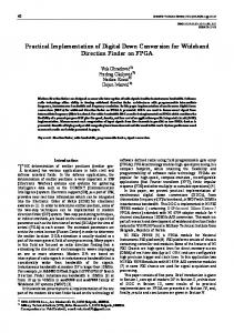
Fig.2. Signals recorded for a toroidal sample of grain-oriented electrical steel, magnetised at 1.55 T and 50 Hz, form factor of Vout diverged by 0.99%; only half-cycle is shown for clarity

Analogue circuits are sometimes preferred in magnetic measurements but they can also act in highly undesirable ways [13]. For instance, Barkhausen noise activity could be partially suppressed by the real-time action of analogue feedback [9]. Digital feedback (DF) is thought to be more robust especially from the viewpoint of self-oscillations [4] and nowadays it is ubiquitous in magnetic measurements [1421]. However, multiple papers on the subject of DF typically do not report sufficient implementation of details. The aim of this paper is to provide such practical information so that the DF can be executed in any programming language. Fig.1. Analogue electronic feedback: a) block diagram of a system with a negative feedback loop, b) implementation with operational amplifier and power amplifier; R1 = R2 = 4.7 kΩ; power supplies and decoupling power supply capacitors are not shown for OP177

The waveforms in Fig. 2 were recorded with an analogue feedback circuit based on OP177 (Fig. 1b) [12]. It should be noted that the distortion in Vout occurs after the

16

2. Digital feedback (DF) The concept of DF closely follows that of the analogue feedback (Fig. 1). The output waveform is compared with the reference waveform and an appropriate correction is applied to the generated waveform in order to reduce any discrepancy. However, DF cannot be implemented in real time for excitation at power frequencies, as this would require extraordinary high processing speed, not commonly

PRZEGLĄD ELEKTROTECHNICZNY, ISSN 0033-2097, R. 93 NR 7/2017

available. Still, for most magnetic measurements real-time operation is not required and full and stable control can be achieved iteratively. The process is somewhat akin to demagnetisation, but applied in the reverse order: the waveforms start from lower amplitude (or zero) and are gradually increased to the target waveform, through all intermediate values (Fig. 3).

have higher permeability at 1.2 T than at 0.1 T. If this is not taken into account then g > 1 can result at some amplitudes of excitation which will inevitably lead to oscillations. Oscillations should be avoided, because they would cause overshooting the target point, and for correct measurements the amplitude should be monotonically increased as required by the international standards [2,3]. Otherwise the sample cannot be treated as demagnetised anymore around the point of interest. The type of operation shown in Fig. 5 is synonymous with a proportional controller. However, the consequence of g < 1 is that the error diminishes exponentially. With each iteration the difference is reduced, but also each applied correction is smaller than the previous. Theoretically it would take infinitely long time to reach 0% error. But in reality the error does not have to be zero, but just smaller than some predefined value e.g. 0.1% and small amplitude corrections can be introduced in the software (for example aiming for a slightly higher amplitude). This makes the convergence time finite and acceptable in practice [19]. DF algorithm can be summarised as shown in the block diagram in Fig. 6.

Fig.3. Maximum target value must pass through all the intermediate values

The algorithm dwells at each amplitude for one or more cycles with magnetising current generated continuously (Fig. 4). 0.3

I (A) 0.2

0.1

distorted cycle

update continuous generation

update

0 0 -0.1

0.05 time 0.1 (s)

0.15

0.2

0.25

0.3

0.35

0.4

0th iteration -0.2

-0.3

1st iteration 2nd iteration

Fig.4. Magnetising current through initial iterations th Before the algorithm starts (0 iteration) the output waveform is zero (generation not started yet) so the difference is equal to 100% of the reference waveform (Fig. 5a). This difference is added with some DF gain g < 1 to the digital output waveform and generated. After the initial 0th iteration there is some output waveform produced but it can be far from the target waveform, due to both g < 1 and nonlinearity of the system (Fig. 5b). In the subsequent iterations the procedure is repeated: acquire, calculate difference, adjust, generate, and so on. With each iteration the controlled signal gets closer to the target waveform.

Fig.5. Iterative operation, just one half-cycle shown Fig.6. Digital feedback algorithm, i – iteration

For a linear system the target could be theoretically achieved in just one iteration by setting g = 1. But in reality there are no ideally linear systems so g < 1 should be set in order to prevent instabilities. For instance, electrical steels

The notation T (bold font) means that the variable is an analogue or digital waveform, whereas Tpeak (normal font) denotes just a single value, peak in this case. The algorithm

PRZEGLĄD ELEKTROTECHNICZNY, ISSN 0033-2097, R. 93 NR 7/2017

17

shown in Fig. 6 should be self-explanatory and can be implemented with the corresponding block diagram shown in Fig. 7.

Fig.7. Block diagram of magnetising setup with DF: R corresponds to Vout and G to Vgen

The diagrams in Fig. 6 and Fig. 7 do not include one information critical for correct DF operation. Namely, proper phase information must be maintained for all the signals (Fig. 8). 3. Triggering For a given target measurement point, the ideal target waveform T (produced just virtually in the software) is kept constant in amplitude and phase. Therefore, the natural approach is to trigger the controlled real waveform Vout (synonymous with the digitised waveform R) to have the same phase as the target waveform T. Then the difference waveform D can be calculated by a direct subtraction of R from T in step 3 (Fig. 6). In a general case there will be a phase shift between the generated and the controlled signal (Fig. 8). The generated signal Vgen has the zero crossings at different points than the triggered signal Vout. This is important because if R (synonymous with Vout) is always triggered then its phase will by definition be the same as that of T. But the generated signal Vgen needs to have its phase shifted accordingly (Fig. 8).

Fig.8. Typical phase relationship for secondary voltage "Vout", flux density "B", and generated voltage "Vgen"

It turns out that the phase of the digital waveform G held in the buffer for generation might not be directly related to the actual phase of the physical generated signal Vout [22,23]. If the phase correlation between the physical voltages cannot be derived from just the digital information inside the software then it will be required to re-measure the justgenerated waveform Vgen.

18

This can be achieved by simply connecting the same signal to the power amplifier input as well as simultaneously to another analogue input (Fig. 7). Then, the previous iteration waveform Gi-1 in step 6 (Fig. 6) becomes the remeasured voltage waveform of Vgen. This completely defines the phase information for all the signals relevant to DF, because T has the arbitrarily set phase, R is triggered to have the same phase as T and G is re-measured with the actual phase difference between R and G. The action of re-measuring Vgen can also introduce minute gain error which is insignificant for DF stability, but can be a nuisance for high-precision convergence. For instance, DF will drive all the signals to very close vicinity of the target value (e.g. Bpeak error < 0.5%) but will be incapable of getting any closer, for infinitely long time. This arises because the analogue output and input channels can introduce small amplitude errors [23] so the acquired Vgen will numerically differ by small amount from the generated Vgen. Small static and/or dynamic amplitude corrections might be required for each input range in such a case. Small jitter due to finite sampling frequency can be eliminated by precise post-triggering [24]. 4. System gain and feedback gain It was mentioned above that the value of DF gain g should be set to less than unity so under all conditions g < 1. However, the multiplier k in Fig. 6 is not synonymous with the total gain g of DF, and in a general case k ≠ g. There are several stages of signal processing, some of which are not immediately obvious from the block diagrams in Fig. 6 and Fig. 7. Some of the values might be difficult to define, e.g. in the case of power amplifier with manually adjustable gain. However, the system gain can be estimated from signal amplitudes. With the DF disabled, some low amplitude sinusoidal signal G (converted to the physical signal Vgen) should be generated, so that the sample is not magnetised above the "knee" in the B-H curve. The signal Vout from the sample measured back as R will also have shape close to sinusoidal. The system gain s can be then estimated from the peak values as s ≈ Rpeak / Gpeak. The overall DF gain is therefore g ≈ k · s and thus the value of k (Fig. 6) should be set as k ≤ g / s. The values estimated in this way can be kept constant from quasi-linear to near saturation excitation. As shown in step 3 (Fig. 6), the difference waveform D is calculated as absolute (in volts) with respect to the peak of the target waveform T. For example, if the system gain was s = 1 then also k =1 could be set in DF, because the input and output voltages of DF would be equal (in the linear operating region). So both the difference D and the correction C can be expressed in volts, and C can be added directly to G in order to produce the new, corrected G. For any different s value the factor k is responsible for scaling the correction waveform to appropriate amplitude in volts. For ensuring g ≤ 1 it should be set that k ≤ 1 / s. The same functionality can be achieved if the differences are calculated not as absolute but relative. Equations in Fig. 6 should be modified accordingly to match the units. It should be stressed that for stable DF operation the value of k must be set correctly for each configuration of the system: changed gain of the power amplifier, turn ratio of the isolating transformer, turn ratio of test windings N2/N1, value of the shunt resistor, etc. Apparatus like Epstein frame or single sheet tester have fixed internal turn ratio, but for a toroidal sample number of turns can vary, and thus the k value must be set accordingly.

PRZEGLĄD ELEKTROTECHNICZNY, ISSN 0033-2097, R. 93 NR 7/2017

5. Universal feedback DF convergence can be accelerated significantly in a number of ways [17-19, 25]. Such methods can be very effective, with as few as just three iterations sufficient for full waveshape control [25]. The main functionality of DF is based on a proportional controller, and the integral and derivative terms can be added as well (PID controller). Even such techniques like artificial neural networks [21] or evolutionary algorithms were utilised [26]. However, such methods are not universal. Any DF using a number of coefficients like the values of resistance and inductance of the primary winding [17] or relying on identification of other additional parameters [18] requires adjustment of all these parameters for each magnetising configuration they are applied to, and perhaps even just for a new sample with much stronger non-linearity, because otherwise there is a risk of instability. In practical applications of DF it is usually sufficient to rely just on the action of the proportional controller, without sophisticated acceleration. This makes DF converge slower, but it can be applied in a truly universal way, without complex adjustment procedures, to a plethora of various magnetising systems: toroidal sample, Epstein frame, single strip tester, rotational yoke, etc. Such universal operation was also demonstrated in [19] where just the proportional action was used. It is only required to change the easily identifiable k value to avoid oscillations. The control of shape of flux density (B) or induced voltage (dB/dt) is synonymous, because if one is controlled precisely so is the other due to their strict mathematical relationship. However, control based on dB/dt (voltage) is more precise because distortions are exaggerated for higher harmonics. Larger relative difference produces larger correction which speeds up convergence. There is also an additional benefit of improved phase margin (discussed below), because B lags exactly 90° behind dB/dt. Proportional-control DF can be used directly for stable control of very complex waveshapes emulating PWM waveforms [19]. For controlling the H waveform [20] the target T must be replaced by an appropriately scaled waveform, and controlled will be some signal proportional to H, e.g. voltage drop across a shunt resistor or an integrated signal from an H-coil. Hence, k must be set to a value which ensures proportionality between the units of A/m and V of the generated voltage Vgen. All other DF components can remain unchanged. 6. Current glitches Operation of DF is based on a single cycle of waveforms (Fig. 8). In a general case the data held in the digital buffers for G, and thus for the generated signal Vgen will not start from zero, but it might have phase as shown in Fig. 8. Continuous generation of waveform is carried out automatically by low-level software and hardware, which repeatedly re-generates analogue voltage from the digital buffer. However, after DF completes an iteration, the output buffer is loaded with some new data, automatically generated. If the new buffer has different amplitude then a sudden glitch or "jump" in the signal will appear (Fig. 9). Such behaviour is clearly visible in a real current waveform in Fig. 4, where the buffer is updated just before the peak value of the waveform. The vertical arrows indicate the time instants when the output buffer is updated and the hardware instantly starts generating new data, with visibly higher amplitude. The amplitude of such glitches is directly proportional to the size of the applied correction. In the worst case, g = 1 could mean 100% jump. In magnetic measurements such sudden jumps should be avoided, so the overall gain of DF

should be set to a value significantly lower than unity, even though many iterations would be executed for convergence. But such approach minimises the amplitude of such current jumps and improves reproducibility of measurements. This is the primary reason why DF acceleration should be avoided, because such techniques increase the correction of initial steps so that the target waveform is achieved in fewer steps. It should be remembered that the fact that current jumps might still occur even if they are not present in the acquired digital waveforms. If acquisition takes place somewhere within the interval of "continuous generation" (Fig. 4) then the waveform would not contain any current jumps, so the user might be unaware of it. It is therefore necessary to investigate the signals by independent methods, e.g. by a standalone oscilloscope. Another practical problem is auto-ranging of analogue input channels. If not executed properly clipping might occur which would disturb DF operation, further exacerbated by acceleration techniques.

Fig.9. Explanation of the mechanism behind current glitches

7. Convergence The condition of achieving the target operating point can be automatically "judged" for example by measuring three quantities simultaneously: form factor error (FF error), total harmonic distortion (THD) and peak flux density error (Bpeak error), although in practice THD and Bpeak error suffice, and the FF error is just measured for compliance with the standards. The convergence curves shown in Fig. 10 were recorded for a toroidal sample of grade M4 (conventional) grain-oriented electrical steel magnetised at 50 Hz from zero to 1.9 T (without intermediate steps).

Fig.10. Convergence for 1.9 T, g = 1, k = 0.4, s = 2.5 (also Fig. 11)

The corresponding waveforms are shown in Fig. 11. The gain was set to g = 1 with controlled sinusoidal voltage (target criteria: FF error < 0.2%, THD < 1%, Bpeak error < 0.1%). Convergence took 1342 iterations and 106 s.

PRZEGLĄD ELEKTROTECHNICZNY, ISSN 0033-2097, R. 93 NR 7/2017

19

However, Bpeak error was reduced to < 3% within first 10 iterations. Therefore, it would be better to start DF with much lower gain (e.g. g < 0.1, or lower) so that the initial convergence is slower with smaller current jumps, and increase to g = 1 after Bpeak error < 3%.

As evident from Fig. 13, the phase reaches the highest delay from all curves, and phase delay above 45° becomes increasingly difficult to control, especially that the gain characteristics droops by a factor greater than 10 at 2.5 kHz (highest controlled harmonic in this case). As mentioned above, direct coupling of power amplifier with the sample resulted with very fast convergence. Such behaviour is supported by the phase and gain characteristics from Fig. 13 – both green curves remain closest to 0° phase or constant gain for all harmonics.

Fig.11. Data measured at controlled sinusoidal 1.9T (also Fig. 10)

With the isolating transformer disconnected, the system gain changed, so that k had to be changed as well to keep g < 1 (in this case it corresponded to k = 0.035). The difference in convergence was remarkable because it took only 68 iterations (6 s) to converge. The comparison between Vgen waveforms for cases with isolating transformer and without it is shown in Fig. 12 (other signals were the same as previously, so are not repeated). It should be noted that the amplitude of the Vgen signal is around 10 times greater for the configuration with isolating transformer. 2

Vgen +TX (V)

0.2

Vgen -TX (V)

with TX without TX

1

0.1

0 0

5

10

15

time (ms)

0 20

-1

-0.1

-2

-0.2

Fig.12. Vgen with (+TX) and without (-TX) the isolating transformer

8. System phase and amplitude characteristics Full analysis of phase shift effects is beyond the scope of this paper. However, any feedback (analogue or digital) requires certain minimum phase margin for stable operation [4,5]. For example, a phase delay of 180° would constitute positive feedback (uncontrollable). Phase and gain characteristics of three typical experimental configurations were measured from 1 Hz to 40 kHz (Fig. 13), between the fundamental harmonics of the generated Vgen and controlled Vout (see also Fig. 8). The system gain varied from 0.30 to 28 (at 50 Hz), which is around a factor of 100. Yet, it was sufficient just to change the k value to obtain stable operation in all cases. The case s = 7.3 took the longest to converge at high excitation.

20

Fig.13. Phase (top) and gain (bottom) characteristics for: s = 28 (k < 0.035) without transformer, s = 7.3 (k < 0.137) with transformer 250:250, and s = 0.30 (k < 3.3) with transformer 250:50; gain curves normalised to 50 Hz

It should be emphasized that if the system phase characteristics exhibits excessive phase delay then in general it will also be unstable for non-proportional controllers. And conversely, even high resistance in the current path will be acceptable with an appropriate phase margin. 9. Multi-channel feedback Two or three magnetising phases might be employed in rotational magnetisation measurements [19]. In such apparatus a separate DF channel would be used for each phase. The channels are magnetically inter-coupled to some degree in the sample, affecting each other signals. But each DF channel sees the other channel as disturbance which will be suppressed by the feedback action. There is no special need to cater for such mutual coupling and correct DF operation can be achieved just by using multiple, independent channels with proportional controllers [16, 19], even for highly anisotropic materials (strong nonlinearity) [27]. However, the phase information must be preserved for all signals, but only one "master" signal can be used for triggering, with all other signals having phases relative to it (for instance signal for channel x or phase A). Multiple Vgen signals must be re-measured (Fig. 7), one for each channel. 10. Instability protection A random external signal glitch might cause incorrect trigger. Also, it will be enough to incorrectly set k to a wrong value to produce uncontrolled and dangerous oscillations, which could instantly demand full power from the amplifier. Such situation can easily arise and thus DF should be protected at least digitally (see "unstable" in Fig. 6). In

PRZEGLĄD ELEKTROTECHNICZNY, ISSN 0033-2097, R. 93 NR 7/2017

practice setting the criterion to THD < 100% in protection is quite useful. Such value indicates large distortion, but usually still small enough for safe operation. Another criterion could be the amplitude of calculated G, just before generation. If this exceeds certain value the operation should stop automatically. Before generation, the output waveform G should be filtered with an "ideal" low-pass filter. The signal can be subjected to Fourier transform, all harmonics above cut-off frequency set to zero, and then re-assembled by inverse Fourier transform. This limits the active harmonics spectrum for DF which improves stability and convergence [19]. Care must be taken to set the cut-off frequency high enough (e.g. 50 harmonics) because otherwise the insufficiently controlled higher harmonics will appear as small ripple in the signals [20]. Measured signals must not be filtered. 11. Summary The components of the main digital feedback algorithm presented here are used in several magnetic measurement laboratories, and personally by the author at: Wolfson Centre for Magnetics at Cardiff University and Megger Instruments Ltd in the United Kingdom, as well as by others in Poland and Italy. The digital feedback algorithm was tested with several magnetising systems: Epstein frame, single strip tester, toroidal sample. The author employed such feedback in his studies of rotational magnetisation, which required simultaneous control of two feedback channels. Also a controlled threephase magnetisation of a transformer was demonstrated. Various materials were tested, from electrical steels through soft ferrites to nanocrystalline cores, at frequencies from at least 0.5 Hz to 100 kHz. The controlled waveforms can be sinusoidal, triangular, trapezoidal, pulse-width modulated or any other shape which can be represented by a bandwidth with sufficient phase and gain margin for the hardware system. Therefore, the digital feedback algorithm presented in this paper were proven to be sufficient for universal operation under various practical dynamic (AC) conditions encountered in magnetic measurement laboratories. The author would like to thank Mr Jeff Jones for his expertise and help with the analogue feedback circuitry. Authors: Dr Stan Zurek, Megger Instruments Ltd, Archcliffe Road, Dover, CT17 9EN, Kent, United Kingdom, [email protected]

REFERENCES [1] [2] [3] [4]

IEC 60404-3:1992 (Single Sheet Tester) IEC 60404-2:1998 (Epstein frame) IEC 60404-6:2003 (Ring specimen) B e c k l e y P . , Electrical steels, European Electrical Steels, Newport, UK, 2000 [5] B a k s h i V.U., B a k s h i U.A., Control System, Technical Publications, 2008

[6] C o x J.F., Fundamentals of Linear Electronics: Integrated and Discrete, Cengage Learning, 2002 [7] M a z z e t t i P., S o a r d o P., Electronic hysteresisgraph holds dB/dt constant, Review of Scientific Instruments, Vol. 37 (5), 1966, p. 548 [8] K u b a c h R.W., A hysteresisgraph for plotting magnetization curves, Dayton University, 1966 [9] B a l d w i n J.A. Jr., A controlled-flux hysteresis loop tracer, Review of Scientific Instruments, Vol. 41, 1970, p. 468 [10] B l u n d e l l M.G., et al., A new method of measuring power loss of magnetic materials under sinusoidal flux conditions, J. Magnetism and Magnetic Materials, Vol. 19, 1980, p. 243 [11] T u m a n s k i S., Handbook of magnetic measurements, CRC Press, 2011 [12] A n a l o g D e v i c e s , Ultraprecision Operational Amplifier, OP177, Data sheet, Rev. G [13] F i o r i l l o F., Measurement and Characterization of Magnetic Materials, Elsevier, 2004 [14] B e r t o t t i G., et al., Loss measurements on amorphous alloys under sinusoidal and distorted induction waveform using a digital feedback technique, J. App. Phys., Vol. 73 (10), 1993, p. 5375 [15] B i r k e l b a c h G . , et al., Very low frequency magnetic hysteresis measurements with well-defined time dependence of the flux density, IEEE Trans. Magnetics, Vol. 23 (5), 1986, p. 505 [16] S p o r n i c S.A., et al., Numerical waveform control for rotational single sheet testers, Journal de Physique IV, Vol. 8 (2), 1998, p. 741 [17] M a t s u b a r a K., et al., Acceleration technique of waveform control for single sheet tester, IEEE Trans. Magnetics, Vol. 31 (6), 1995, p. 3400 [18] M a k a v e e v D., et al., Waveform control algorithm for rotational single sheet testers using system identification techniques, J. Applied Physics, Vol. 87 (9), 2000, p. 5983 [19] Z u r e k S., et al., Use of novel adaptive digital feedback for magnetic measurements under controlled magnetising conditions, IEEE Trans. Magnetics, Vol. 41 (11), 2005, p. 4242 [20] Z u r e k S., et al., Adaptive iterative digital feedback algorithm for measurements of magnetic properties under controlled magnetising conditions over a wide frequency range, Przeglad Elektrotechniczny, R. 81, Nr 12/2005, 2005, p. 5 [21] B a r a n o w s k i S., et al., Comparison of digital feedback methods of the control of flux density shape, Przeglad Elektrotechniczny, R. 85, Nr 1/2009, 2009, p. 93 [22] Z u r e k S., private correspondence with Technical Support of National Instruments, 2015 [23] N a t i o n a l I n s t r u m e n t s , NI USB-621x User Manual, 2009 [24] Z u r e k S., et al., Correction of triggering and interchannel delay in alternating and two-dimensional measurements of magnetic properties, Przeglad Elektrotechniczny, Nr 5/2005, p. 78 [25] A n d e r s o n P., A universal DC characterisation system for hard and soft magnetic materials, J. Magnetism and Magnetic Materials, Vol. 320 (20), 2008, e589 [26] M e h n e n L., et al., 2D magnetisation control by means of evolutionary algorithms, Proceedings of 6th 1&2DM Workshop, 2000, Bad Gastein, Austria, p. 122 [27] Z u r e k S., Example of vanishing anisotropy at high rotational magnetisation of grain-oriented electrical steel, presented at Symposium of Magnetic Measurements & Modeling, Czestochowa – Siewierz, Poland, 2016

PRZEGLĄD ELEKTROTECHNICZNY, ISSN 0033-2097, R. 93 NR 7/2017

21