OCA variable combinations and reported the successful ones in a sense that they produced either similar or better results than those of Ozer and Ozkan's (2007) ...
SCIENTIFIC PAPERS
Itir Ozer and Ibrahim Ozkan*
DOI: 10.2298/EKA0876038O
PRACTICAL INSIGHTS FROM OCA VARIABLE COMBINATIONS ABSTRACT: This study aims to identify optimum currency areas (OCA) variables that distinguish certain Economic and Monetary Union (EMU) member countries from the other EMU members. In the previous studies, EMU members were identified in the light of criteria suggested by the OCA theory. In this study, in order to obtain additional insights, we analysed OCA variables and the performance of
JEL CLASSIFICATION: F15, C82
*
38
Hacettepe University, Ankara, Turkey
European countries with respect to these variables. Our analysis shows that some of the EMU member countries are dissimilar to the rest of the EMU members with respect to certain OCA criteria. KEY WORDS: optimum currency areas, fuzzy C-means clustering, EMU, HodrickPrescott filtering technique
INSIGHTS FROM OCA VARIABLES
1. Introduction
Optimum currency areas (OCA) theory aims to determine the appropriate domain of a currency area. Starting from the 1960s, optimality of a currency area has been defined in terms of several criteria in the pioneering phase of the OCA theory. Mobility of factors of production (Mundell, 1961), the degree of economic openness (McKinnon, 1963), product diversification (Kenen, 1969), the degree of financial integration (Ingram, 1969), similarity of inflation rates (Haberler, 1970 and Fleming, 1971) and the degree of policy integration (Tower and Willet, 1970) are the criteria put forward in the pioneering phase1. This study aims to identify OCA variables that distinguish certain Economic and Monetary Union (EMU) member countries and it is based on the studies of Ozer et al. (2007) and Ozer and Ozkan (2007). In the OCA theory literature, industrial production series and the real interest rates have been detrended with the Hodrick-Prescott (H-P) filter2 with the smoothing parameter set at 50,000 in the calculation of synchronisation in business cycles and synchronisation in the real interest rates. Ozer et al. (2007) and Ozer and Ozkan (2007) applied both the Hodrick-Prescott and the Baxter-King (B-K)3 filters to industrial production series and the real interest rates, and showed that the application of different filtering techniques produces different results for the same data set, and hence results are highly sensitive to the filtering techniques employed. Besides, Ozer and Ozkan (2007) employed fuzzy c-means (FCM) clustering to the criteria suggested by the OCA theory, and used the levels of fuzziness of 1.4 and 2.6 as lower and upper levels of fuzziness, respectively, determined by Ozkan and Turksen (2007). They demonstrated that for the level of fuzziness of 1.4, Turkey and Romania, and the control group countries, Canada and Japan are grouped in two separate
1
2 3
For studies in the reconciliation phase of the OCA theory see: Fleming (1971), Corden (1972), Ishiyama (1975) and Tower and Willet (1976); for contributions in the reassessment phase see: Artis (1991), Tavlas (1993), Tavlas (1994), Mélitz (1991), Giavazzi and Giovannini (1989), Krugman (1991), Krugman (1993) and Bertola (1989); for econometric studies see: Coenen and Wieland (2000), Smets and Wouters (2002) and Banerjee et al. (2005), and for studies based on techniques of pattern recognition see: Eichengreen (1991), Bayoumi and Eichengreen (1992), Eichengreen and Bayoumi (1996), Artis and Zhang (2001), Artis and Zhang (2002), Alesina et al. (2002), Boreiko (2002), Komárek et al. (2003), and Kozluk (2005). Finally, for an overall assessment of the OCA theory see: Mongelli (2002). See Hodrick and Prescott (1997). See Baxter and King (1999).
39
Itir Ozer and Ibrahim Ozkan
clusters when the number of clusters is four in the analysis with the H-P filter4 and when the number of clusters is five in the analysis with the B-K filter. The analysis with the H-P filter produced better results both for the levels of fuzziness of 1.4 and 2.6. When the level of fuzziness is 1.4 (close to crisp clustering), Cluster I contains seventeen countries, twelve of which are EMU members, whereas the EMU member countries, Greece, Portugal and Slovenia are in Cluster II. Canada and Japan, and Turkey and Romania form separate clusters labelled as Cluster III and Cluster IV respectively. It was concluded then that the OCA theory provides quite sensible results when FCM clustering technique is applied to the OCA criteria obtained by the appropriate H-P filter. Since economic variables are interrelated and the clustering methodology is an unsupervised non-linear technique, we applied FCM clustering to all possible OCA variable combinations and reported the successful ones in a sense that they produced either similar or better results than those of Ozer and Ozkan’s (2007). Through these means, we demonstrated the OCA variables distinguishing certain EMU member countries. The remainder of the paper is organised as follows. In section 2, data and methodology are briefly discussed. In section 3, the results are provided. Finally, section 4 concludes the study.
2. Data and Methodology 2.1. OCA Criteria
Following Artis and Zhang (2001), Boreiko (2003) and Kozluk (2005), the OCA variables have been computed as follows and similarly it has been assumed that Germany is the centre country5. 1) Synchronisation in business cycles has been represented by the cross-correlation of the cyclical components of deseasonalised industrial production series, detrended with an application of the Hodrick-Prescott (H-P) filter. The smoothing parameter has been set at 50,000 following Artis and Zhang (2001) and Boreiko (2003). The cross-correlations have been measured for all the countries in the 4
5
40
In this case, they set the smoothing parameter’s value at 50,000 following Artis and Zhang (2001), Artis and Zhang (2002) and Boreiko (2002) for industrial production series. However, different from the OCA theory literature, they detrended the real interests with the H-P filter in which the optimum smoothing parameters have been calculated, based on the nature of the time series data (Dermoune et al., 2006: 2-4) following Schlicht (2005). Frequency, data sources and the time interval of the data are given in Appendix A.
INSIGHTS FROM OCA VARIABLES
sample, with reference to the centre country, Germany. Since correlation results in values between –1 and +1 inclusive, correlation values have been subtracted from one, so the new values are between zero and two. Zero represents perfect positive correlation (perfect synchronisation), and two represents perfect negative correlation. 2) Volatility in the real exchange rates has been represented by the standard deviation of the log-difference of real bilateral DM exchange rates before 1999. After 1999, the Euro has been used instead of DM exchange rates. Real exchange rates have been obtained by deflating nominal rates by relative wholesale/producer price indices6. 3) Synchronisation in the real interest rates has been represented by the crosscorrelation of the cyclical components of the real interest rate cycle of a country with that in Germany. Real interest rates have been obtained by deflating shortterm nominal rates by consumer price indices. Then, they have been detrended with the H-P filter in which the optimum smoothing parameters have been calculated, based on the nature of the time series data (Dermoune et al., 2006: 2-4) following Schlicht (2005). Cross-correlations have been measured for all the countries in the sample with reference to Germany, and again the values have been set between zero and two. 4) The degree of trade integration has been measured by , where xi and mi are exports and imports (of goods) respectively, of country i, and superscript EU-25 represents European Union countries as of May 2004. 5) Convergence of inflation has been measured by ei-eg, where ei and eg are the rates of inflation in country i and Germany, respectively. The calculated values of the OCA variables to which the FCM clustering algorithm has been applied are given in Table 1.
6
For Portugal, consumer price index has been used because of the lack of data.
41
Itir Ozer and Ibrahim Ozkan
Table 1. OCA Variablesa Synchro- Volatility Synchroni- The Degree Conver nisation in the sation of gence in Real in the Real Trade Inteof d Business Exchange Interest gration Inflatione b c b Cycles Rates Rates Austria 0.0965 0.0046 0.3633 76.38 0.3436 Belgium 0.2821 0.0121 0.5183 75.52 0.8296 Croatia 0.9736 0.0253 1.6042 67.49 1.3846 Cyprus 0.8874 0.0047 0.4384 63.82 0.6046 Czech Republic 0.9351 0.0129 1.2068 80.03 -0.1080 Denmark 0.4276 0.0046 0.0497 70.49 -0.1454 Finland 0.2459 0.0044 0.5648 62.00 -1.0923 France 0.4427 0.0028 0.5049 66.83 -0.2098 Greece 0.3882 0.0047 1.1608 57.33 1.6073 Hungary 0.1536 0.0206 1.4870 75.27 1.5975 Ireland 0.6647 0.0046 0.6415 62.75 0.4617 Italy 0.4642 0.0031 0.5366 59.61 0.0313 Luxembourg 0.5957 0.0111 0.2620 81.54 0.5360 Netherlands 0.6107 0.0042 0.4927 66.98 -0.2906 Norway 0.7397 0.0342 0.2538 75.46 -0.4319 Poland 0.3994 0.0261 0.3448 76.36 0.1528 Portugal 1.1110 0.0053 0.5307 78.20 0.3397 Romania 0.9328 0.0338 0.5271 71.61 7.0354 Slovak Republic 0.6833 0.0145 1.3264 83.13 0.7549 Slovenia 0.3025 0.0067 0.8753 74.16 0.5250 Spain 0.5056 0.0033 0.2794 69.25 1.4138 Sweden 0.4373 0.0123 0.3722 67.49 -1.5007 Turkey 0.5966 0.0672 0.4547 49.81 6.2252 United Kingdom 0.3170 0.0161 1.0504 53.38 0.8768 Canada 0.3371 0.0241 0.4975 8.38 0.2802 Japan 0.3931 0.0252 1.0198 14.43 -2.2271 The values of OCA variables for Germany are not given in Table 1 since Germany is the centre country. For Germany, the only variable that is different from zero is the degree of trade integration and it is equal to 62.96. b Values are between zero and two, where zero represents perfect synchronisation. c Volatility in the real exchange rates has been calculated for the values after January 1999. d The degrees of trade integration are calculated from 2004 data. e Convergence of inflation values are calculated from 2005 data. a
42
INSIGHTS FROM OCA VARIABLES
Following Ozer et al. (2007), the principal component analysis (PCA) has been employed in order to gain insight on the structure of the data. As a result of the PCA analysis, it has been observed that the first, second and third principal components explain 35.88 %, 25%, and 19.97 % of the variability in the data, respectively. Two of the figures, that of importance demonstrating the structure of the data, are presented in Figures 1a and 1b. Figure 1a. 1st and 2nd Principal Components
43
Itir Ozer and Ibrahim Ozkan
Figure 1b. 1st and 3rd Principal Components
As it can be observed in Figure 1a, Canada and Japan are distinguished from the European countries and form their own cluster. In Figure 1b, Turkey and Romania are far from the European countries and form their separate cluster. Therefore, the performance of our analysis can be assessed by means of the following: 1. Canada and Japan forming their own cluster, 2. Turkey and Romania forming their separate cluster, 3. At least twelve of the EMU members being in the same cluster7. 7
44
Malta and Cyprus became EMU members in January 2008 and there are now fifteen countries in the Euro area. We excluded Malta from the sample because of the lack of data for industrial production series and although Cyprus is in our sample, we did not include Cyprus in the EMU cluster as it is a new member and is a very small country relative to the other members. Therefore, although there are fifteen countries in the Euro area, identifying at least twelve of them in the same cluster has been assumed as a performance criterion.
INSIGHTS FROM OCA VARIABLES
To this end, we applied FCM clustering algorithm to all possible OCA variable combinations between two and four. In addition, we set the number of clusters to four, and the levels of fuzziness to 1.4, 2 and 2.6. 2.2. Fuzzy C-Means Clustering
Fuzzy c-means (FCM) clustering partitions data into clusters in which each country is assigned a membership value between zero and one to each cluster. The membership values indicate the degree of belongingness of each country to each of the clusters. As the membership value gets higher, the degree of belongingness increases. Bezdek (1973) showed that in the minimisation of the objective function;
(1)
where, mc,k is the membership value of kth vector in cth cluster such that mc,k∈ [0,1], nd is the number of vectors, nc is the number of clusters, ǁ ǁA is norm8 and m is the level of fuzziness, the membership function is calculated as:
where,
(2)
for some given m>1.
3. Results
The cases in which at least twelve EMU members are identified in the same cluster are given in Table 2.
8
This is the similarity measure. After standardizing the OCA variables following Artis and Zhang (2001), Boreiko (2002) and Kozluk (2005), we have employed Euclidian distance as a similarity measure. The Euclidian distance between country i and country j is given as:
45
Itir Ozer and Ibrahim Ozkan
Table 2. EMU Members Identified in Clusters Level Variable comof binationa fuzziness 1 and 2 1 and 2 2 and 3 2 and 3 2 and 3 2 and 4 2 and 5 2 and 5 2 and 5 2, 3 and 4 2, 3 and 4 2, 3 and 4 2, 3 and 5 2, 3 and 5 2, 3 and 5 2, 4 and 5 2, 4 and 5 3, 4 and 5 2, 3, 4 and 5 2, 3, 4 and 5
2 2.6 1.4 2 2.6 1.4 1.4 2 2.6 1.4 2 2.6 1.4 2 2.6 1.4 2 1.4 1.4 2
Number of EMU members identified 12 (Portugal)b 12 (Portugal) 12 (Greece) 12 (Greece) 12 (Greece) 12 (Luxembourg) 13 13 12 (Belgium) 12 (Greece) 13 13 12 (Greece) 13 12 (Luxembourg) 12 (Luxembourg) 12 (Luxembourg) 12 (Greece) 12 (Greece) 13
Number of countries in the cluster 15 15 15 15 15 16 20 15 14 15 17 17 14 15 15 15 16 17 17 17
Position Position of the of control Turkey group – – – – – + – – – + + + – – – + + + + +
– – – – – – – + + – – – + + – + + + + –
Notes: Number of clusters is 4 a 1 represents synchronisation in business cycles. 2 represents volatility in the real exchange rates. 3 represents synchronisation in the real interest rates. 4 represents the degree of trade integration. 5 represents convergence of inflation. b Countries given in bold and parenthesis are the EMU member countries remaining outside of the cluster of the other EMU members.
The first column presents the OCA variable combinations for the EMU member countries and the forth column shows the number of countries in the cluster, to 46
INSIGHTS FROM OCA VARIABLES
which the EMU members belong. In the fifth column, + denotes that the control group, Canada and Japan form their separate cluster, whereas – indicates that they are either in different clusters or in the same cluster with the European countries. For the position of Turkey (the sixth column), + denotes that it forms a separate cluster with Romania, whereas – indicates that it is in the same cluster with the European countries. For different variable combinations Portugal, Greece, Luxembourg and Belgium are in different clusters than the other EMU member countries. Belgium is in a different cluster when the FCM clustering technique is applied to volatility in the real exchange rates (2) and convergence of inflation (5) combination and the value of level of fuzziness is set to 2.6. Since clusters highly overlap when the value of the level of fuzziness is high, this result is expected. Indeed, for the same combination all of the EMU members are identified in the same cluster for lower values of levels of fuzziness of 1.4 and 2. Therefore, it can be stated that in all cases, Belgium has been identified as a member of the EMU cluster. Portugal
Portugal remains in a separate group than the other EMU member countries when synchronisation in business cycles (1) is included. Therefore, it can be asserted that Portugal’s similarity to the centre country, Germany, with respect to synchronisation in business cycles is low. The cross-correlation of the cyclical components of industrial production series between Germany and Portugal are given in Figure 2a, whereas cyclical components of industrial production series of Germany and Portugal are given in Figure 2b.
47
Itir Ozer and Ibrahim Ozkan
Figure 2a. �Cross-correlation, Industrial Production Series, Germany and Portugal
Figure 2b. Cyclical Components of Production Series of Germany and Portugal
48
INSIGHTS FROM OCA VARIABLES
As it can be observed from the Figures 2a and 2b, the correlation in business cycles is very low with a lag of zero month and the correlation gets its maximum value with a lag of approximately one year. Greece
When synchronisation in the real interest rates (3) is included, Greece cannot be identified in the same cluster with the other EMU members. The cross-correlation of the real interest rates of Germany and Greece are given in Figure 3a, whereas cyclical components of real interest rates of Germany and Greece are given in Figure 3b. According to Figures 3a and 3b, Greece’s real interest rates are more volatile when compared to Germany and the cross-correlation of real interest rates are low with a lag of zero month. Therefore, Greece’s real interest rates do not exhibit synchronisation with those of Germany. Figure 3a. Cross-correlation of Real Interest Rates of Germany and Greece
49
Itir Ozer and Ibrahim Ozkan
Figure 3b. Cyclical Components of Real Interest Rates of Germany and Greece
Luxembourg
Luxembourg remains in a different cluster than the other EMU members when volatility in the real exchange rates (2) and the degree of trade integration (4) are included in the combinations. Luxembourg’s degree of trade integration is 81.54. The minimum, maximum and mean values of the degree of trade integration for the EMU members are 57.33, 81.54 and 68.73, respectively. Box-plot of the degree of trade integration of the EMU members is given in Figure 4. It can be seen that Luxembourg’s degree of trade integration has the highest value. Therefore, this value explains Luxembourg remaining outside of the EMU cluster, although it has better trade integration with the European Union (EU).
50
INSIGHTS FROM OCA VARIABLES
Figure 4. Box-plot of the Degree of Trade Integration
4. ConclusIon
This study aims to identify OCA variables that distinguish certain EMU member countries. According to our results, thirteen EMU members are identified in the same cluster in six different variable combinations. Among those, in two combinations: volatility in the real exchange rates (2) and convergence of inflation (5); and volatility in the real exchange rates (2), synchronisation in the real interest rates (3) and convergence of inflation (5), there are fifteen countries in the cluster when the value of the level of fuzziness is 2. These two combinations seem to give the best results. However, in these combinations, Canada and Japan do not form their separate clusters. The cases in which both the control groups, Canada and Japan, and Turkey and Romania form their separate clusters are: i) volatility in the real exchange rates (2), the degree of trade integration (4) and convergence of inflation (5) when the levels of fuzziness are 1.4 and 2, 51
Itir Ozer and Ibrahim Ozkan
ii) synchronisation in the real interest rates (3), the degree of trade integration (4) and convergence of inflation (5) when the level of fuzziness is 1.4, iii) volatility in the real exchange rates (2), synchronisation in the real interest rates (3), the degree of trade integration (4) and convergence of inflation (5) when the level of fuzziness is 1.49. Convergence of inflation (5) distinguishes Turkey and Romania. Besides, Turkey’s degree of trade integration (4) is low. Luxembourg, Greece and Portugal’s performances are different than the other EMU members with respect to the degree of trade integration (4), synchronisation in the real interest rates (3) and synchronisation in business cycles (1), respectively. Portugal’s synchronisation of business cycles with Germany, and Greece’s synchronisation of real interest rates with Germany are low. However, Luxembourg’s degree of trade integration with the EU has the highest value in the sample. This value causes a divergence from the other EMU members. In the light of this analysis, it can be concluded that all OCA variables should be taken into consideration in order to meet the performance criteria we set in Section 2.1, and this type of analysis is suitable to gain insights concerning the performance of the European countries for different OCA variables. 5. Appendices 5.1. Appendix A OCA Variables
Table A-1. Frequency, Data Sources and the Time Interval of the OCA Variables Industrial production series Real exchange rates Real interest rates
Frequency Data Sources monthly IFS
Time Interval 1996:1-2005:6
monthly monthly
1991:1-2006:12 1997:2-2006:10
Trade data
annual
Inflation data
annual
9
52
IFS, TURKSTAT IFS, EUROSTAT, Central Bank of Luxembourg UNCTAD; Handbook of Statistics Online WDI
2004 2005
The cluster members for these combinations are given in Appendix B and the cluster members for all possible variable combinations are available from the authors upon request.
INSIGHTS FROM OCA VARIABLES
The interest rates in Table A-2 have been used for the countries in the sample. Table A-2. Interest Rates Austria Belgium Croatia Cyprus Czech Republic Denmark Finland France Germany
: Government Bond Yield : Government Bond Yield : Money Market Rate : Deposit Rate : Money Market Rate : Call Money Rate : Government Bond Yield : Government Bond Yield : Call Money Rate
Netherlands Norway Poland Portugal Romania Slovak Republic Slovenia Spain Sweden
Greece
: Government Bond Yield
Turkey
Hungary Ireland Italy Luxembourg
: Treasury Bill Rate : Government Bond yield : Money Market Rate : Government Bond Yield
United Kingdom Canada Japan
: Government Bond Yield : Government Bond Yield : Money Market Rate : Government Bond Yield : NBR Structural Credit Rate : Average Lending Rate : Money Market Rate : Call Money Rate : Call Money Rate : �Interbank Money Market Rate : Government Bond Yield : Bank Rate : Government Bond Yield
5.2. Appendix B
Table B-1. Cluster Members for Variable Combination 2 and 5 when m=1.4a EMU Members Identified: 13 Austria, Belgium, Croatia, Cyprus, Czech Republic, Denmark, Finland, France, Germany, Greece, Hungary, Ireland, Italy, Luxembourg, Cluster 1 Netherlands, Portugal, Slovak Republic, Slovenia, Spain, United Kingdom Cluster 2 Croatia, Norway, Poland, Sweden, Canada, Japan Cluster 3 Romania Cluster 4 Turkey a
m=level of fuzziness
53
Itir Ozer and Ibrahim Ozkan
Table B-2. Cluster Members for Variable Combination 2 and 5 when m=2 EMU Members Identified: 13 Cluster 1 Austria, Belgium, Cyprus, Denmark, Finland, France, Germany, Greece, Ireland, Italy, Luxembourg, Netherlands, Portugal, Slovenia, Spain Cluster 2 Norway, Poland, Sweden, Canada, Japan Cluster 3 Belgium, Croatia, Czech Republic, Finland, Greece, Hungary, Luxembourg, Romania, Slovak Republic, Sweden, United Kingdom, Canada Cluster 4 Romania, Turkey Table B-3. Cluster Members for Variable Combination 2 and 5 when m=2.6 EMU Members Identified: 12 Cluster 1 Austria, Cyprus, Denmark, Finland, France, Germany, Greece, Ireland, Italy, Luxembourg, Netherlands, Portugal, Slovenia, Spain Cluster 2 Croatia, Norway, Poland, Sweden, Canada, Japan Cluster 3 Belgium, Croatia, Czech Republic, Finland, Greece, Hungary, Luxembourg, Netherlands, Romania, Slovak Republic, Spain, Sweden, United Kingdom Cluster 4 Romania, Turkey Table B-4. Cluster Members for Variable Combination 2, 3 and 5 when m=1.4 EMU Members Identified: 12 Cluster 1 Austria, Belgium, Cyprus, Denmark, Finland, France, Germany, Ireland, Italy, Luxembourg, Netherlands, Portugal, Slovenia, Spain Cluster 2 Norway, Poland, Sweden, Canada, Japan Cluster 3 Croatia, Czech Republic, Greece, Hungary, Slovak Republic, Slovenia, United Kingdom Cluster 4 Romania, Turkey
54
INSIGHTS FROM OCA VARIABLES
Table B-5. Cluster Members for Variable Combination 2, 3 and 5 when m=2 EMU Members Identified: 13 Cluster 1 Austria, Belgium, Cyprus, Denmark, Finland, France, Germany, Greece, Ireland, Italy, Luxembourg, Netherlands, Portugal, Slovenia, Spain Cluster 2 Norway, Poland, Sweden, Canada, Japan Cluster 3 Croatia, Czech Republic, Greece, Hungary, Slovak Republic, Slovenia, United Kingdom, Japan Cluster 4 Romania, Turkey Table B-6. Cluster Members for Variable Combination 2, 3 and 5 when m=2.6 EMU Members Identified: 12 Cluster 1 Austria, Belgium, Cyprus, Denmark, Finland, France, Germany, Greece, Ireland, Italy, Netherlands, Portugal, Romania, Slovenia, Spain Cluster 2 Austria, Belgium, Cyprus, Denmark, Finland, Germany, Luxembourg, Netherlands, Romania, Spain Cluster 3 Croatia, Czech Republic, Greece, Hungary, Slovak Republic, United Kingdom Cluster 4 Norway, Poland, Sweden, Turkey, Canada, Japan Table B-7. Cluster Members for Variable Combination 2, 4 and 5 when m=1.4 EMU Members Identified: 12 Cluster 1 Canada, Japan Cluster 2 Austria, Belgium, Cyprus, Denmark, Finland, France, Germany, Greece, Ireland, Italy, Netherlands, Portugal, Slovenia, Spain, United Kingdom Cluster 3 Belgium, Croatia, Czech Republic, Hungary, Luxembourg, Norway, Poland, Slovak Republic, Sweden Cluster 4 Romania, Turkey
55
Itir Ozer and Ibrahim Ozkan
Table B-8. Cluster Members for Variable Combination 2, 4 and 5 when m=2 EMU Members Identified: 12 Cluster 1 Canada, Japan Cluster 2 Austria, Belgium, Cyprus, Denmark, Finland, France, Germany, Greece, Ireland, Italy, Netherlands, Portugal, Slovenia, Spain, Sweden, United Kingdom Cluster 3 Austria, Belgium, Croatia, Czech Republic, Finland, Hungary, Luxembourg, Norway, Poland, Portugal, Slovak Republic, Sweden Cluster 4 Romania, Turkey Table B-9. Cluster Members for Variable Combination 3, 4 and 5 when m=1.4 EMU Members Identified: 12 Cluster 1 Canada, Japan Cluster 2 Austria, Belgium, Cyprus, Denmark, Finland, France, Germany, Ireland, Italy, Luxembourg, Netherlands, Norway, Poland, Portugal, Slovenia, Spain, Sweden Cluster 3 Croatia, Czech Republic, Greece, Hungary, Slovak Republic, Slovenia, United Kingdom Cluster 4 Romania, Turkey Table B-10. �Cluster Members for Variable Combination 2, 3, 4 and 5 when m=1.4 EMU Members Identified: 12 Cluster 1 Canada, Japan Cluster 2 Austria, Belgium, Cyprus, Denmark, Finland, France, Germany, Ireland, Italy, Luxembourg, Netherlands, Norway, Poland, Portugal, Slovenia, Spain, Sweden Cluster 3 Croatia, Czech Republic, Greece, Hungary, Slovak Republic, Slovenia, United Kingdom Cluster 4 Romania, Turkey
56
INSIGHTS FROM OCA VARIABLES
Table B-11. Cluster Members for Variable Combination 2, 3, 4 and 5 when m=2 EMU Members Identified: 13 Cluster 1 Canada, Japan Cluster 2 Austria, Belgium, Cyprus, Denmark, Finland, France, Germany, Greece, Ireland, Italy, Luxembourg, Netherlands, Portugal, Romania, Slovenia, Spain, United Kingdom Cluster 3 Luxembourg, Norway, Poland, Sweden, Turkey Cluster 4 Croatia, Czech Republic, Greece, Hungary, Romania, Slovak Republic, Slovenia, United Kingdom
REFERENCES
Alesina, A., Barro, R. J. and Tenreyno, S. (2002), “Optimal Currency Area”, NBER Working Paper No. 9072. Artis, M. J. (1991), “One Market, One Money: An Evaluation of the Potential Benefits and Costs of Forming an Economic and Monetary Union”, Open Economies Review, 2, 315-321. Artis, M. J. and Zhang, W. (2001), “Core and Periphery in EMU: A Cluster Analysis”, Economic Issues, 6(2), 39-60. Artis, M. J. and Zhang, W. (2002), “Membership of EMU: A Fuzzy Clustering Analysis of Alternative Criteria”, Journal of Economic Integration, 17(1), 54-79. Banerjee, A., Marcellino, M. and Masten, I. (2005), “Forecasting Macroeconomic Variables For The New Member States Of The European Union”, ECB Working Paper Series, Working Paper No. 482. Baxter, M. and King, R. G. (1999), “Measuring business cycles: Approximate band-pass filters”, The Review of Economics and Statistics, 81(4), 575-93. Bayoumi, T. and Eichengreen, B. (1992), “Shocking Aspects of European Monetary Unification”, NBER Working Paper Series, Working Paper 3949.
57
Itir Ozer and Ibrahim Ozkan Bertola, G. (1989), “Factor Flexibility, Uncertainty and Exchange Rate Regimes” in A European Central Bank? Perspectives on Monetary Unification After Ten Years of the EMS edited by De Cecco and A. Gioviannini, Cambridge University Press. Bezdek, J. C. (1973), Fuzzy Mathematics in Pattern Recognition, Ph. D. Thesis, Applied Mathematics Centre, Ithaca: Cornell University. Boreiko, D. (2002), “EMU and Accession Countries: Fuzzy Cluster Analysis of Membership”, Oesterreichische Nationalbank Working Paper No. 71. Coenen, G. and Wieland, V. (2000), “A Small Estimated Euro Area Model With Rational Expectations And Nominal Rigidities”, ECB Working Paper Series, Working Paper No. 30. Corden, W. M. (1972), Monetary Integration, Essays in International Finance, No. 93, Princeton, New Jersey: Princeton University. Dermoune, A., Djehiche, B. and Rahmania, N. (2006), “Consistent estimators of the smoothing parameter in the Hodrick-Prescott filter”, Preprint. Eichengreen, B. (1991), “Is Europe an Optimum Currency Area?” NBER Working Paper Series, Working Paper 3579. Eichengreen, B. and Bayoumi, T. (1996), “Ever Closer to Heaven? An Optimum-Currency-Area Index for European Countries”, Institute of Business and Economic Research Centre for International and Development Economics Research Paper C96-078, Berkeley: University of California. Fleming, M. J. (1971), “On Exchange Rate Unification”, Economic Journal, 81, 467-488. Giavazzi, F. and Giovannini, A. (1989), Limiting Exchange Rate Flexibility: the European Monetary System, Cambridge, Massachusetts: The MIT Press. Haberler, G. (1970), “The International Monetary System: Some Recent Developments and Discussions” in Approaches to Greater Flexibility of Exchange Rates: The Bürgenstock Papers, edited by N. H. George, Princeton, N. J.: Princeton University Press, 115-123. Hodrick, R. J. and Prescott, E. C. (1997), “Postwar U.S. business cycles: An empirical investigation”, Journal of Money, Credit, and Banking, 29(1), 1-16. Ingram, J. C. (1969), “Comment: The Currency Area Problem” in Monetary Problems of the International Economy, edited by R.A. Mundell and A.K. Swoboda, Chicago: University of Chicago Press, 95-100. Ishiyama, Y. (1975), “The Theory of Optimum Currency Areas: A Survey”, IMF Staff Papers, XXII, 344-383.
58
INSIGHTS FROM OCA VARIABLES Kenen, P. B. (1969), “The Theory of Optimal Currency Areas: An Eclectic View”, in Monetary Problems of the International Economy, edited by R.A. Mundell and A.K. Swoboda, Chicago: University of Chicago Press, 41-60. Komárek, L., Cech, Z. and Horváth, R. (2003), “Optimum Currency Area Indices – How Close is the Czech Republic to the Eurozone?” The Czech National Bank Working Paper No. 10. Kozluk, T. (2005), “CEEC Accession Countries and the EMU: An Assessment of Relative Suitability and Readiness for Euro-Area Membership”, Journal of Economic Integration, 20(3), 439-74. Krugman, P. R. (1991), “Increasing Returns and Economic Geography”, Journal of Political Economy, 99(3), 483-499. Krugman, P. R. (1993), “Lessons of Massachusetts for EMU” in Adjustment and Growth in the European Monetary Union edited by F. Torres and F. Giavazzi, Cambridge University Press, 241-269. McKinnon, R. I. (1963), “Optimum Currency Areas”, American Economic Review, 53, 717-724. Mélitz, J. (1991), “A Suggested Reformulation of the Theory of Optimal Currency Areas”, CEPR Discussion Papers 590. Mongelli, F. P. (2002), “ ‘New’ Views on the Optimum Currency Area Theory: What is EMU Telling Us?”, ECB Working Paper No. 138. Mundell, R. A. (1961), “A Theory of Optimal Currency Areas”, American Economic Review, 51, 657-65. Ozer, I. and Ozkan, I. (2007), “Optimum filtering for optimum currency areas criteria”, Economics Bulletin, 6(44), 1-18. Ozer, I., Ozkan, I. and Aktan, O. H. (2007), “Optimum Currency Areas Theory: An Empirical Application to Turkey”, South East European Journal of Economics and Business, 2(2), 75-88. Ozkan, I. and Turksen, I. B. (2007), “Upper and Lower Valued for the Level of Fuzziness in FCM” in Fuzzy Logic, A Spectrum of Theoretical and Practical Issues Series: Studies in Fuzziness and Soft Computing, edited by P. P.Wang, D. Ruan and E. E. Kerre, Springer, 215(16), ss. 85-105. Schlicht, E. (2005), “Estimating the Smoothing Parameter in the So-called Hodrick-Prescott Filter”, Journal of the Japan Statistical Society, 35(1), 99-119. Smets, F. and Wouters, R. (2002), “An Estimated Stochastic Dynamic General Equilibrium Model of the Euro Area”, ECB Working Paper Series, Working Paper No. 171.
59
Itir Ozer and Ibrahim Ozkan Tavlas, G. S. (1993), “The ‘New’ Theory of Optimum Currency Areas”, The World Economy, 16(6), 663-685. Tavlas, G. S. (1994), “The Theory of Monetary Integration”, Open Economies Review, 5(2), 211-230. Tower, E. and Willet, T. D. (1970), “The Concept of Optimum Currency Areas and the Choice Between Fixed and Flexible Exchange Rates” in Approaches to Greater Flexibility of Exchange Rates: The Bürgenstock Papers, edited by N. H. George, Princeton, N. J.: Princeton University Press, 407-415. Tower, E. and Willet, T. D. (1976), “The Theory of Optimum Currency Areas and ExchangeRate Flexibility”, Special Papers in International Economics, Princeton, New Jersey: Princeton University Press.
60